HAL Id: hal-01865371
https://hal.archives-ouvertes.fr/hal-01865371
Submitted on 31 Aug 2018
HAL is a multi-disciplinary open access
archive for the deposit and dissemination of
sci-entific research documents, whether they are
pub-lished or not. The documents may come from
teaching and research institutions in France or
L’archive ouverte pluridisciplinaire HAL, est
destinée au dépôt et à la diffusion de documents
scientifiques de niveau recherche, publiés ou non,
émanant des établissements d’enseignement et de
recherche français ou étrangers, des laboratoires
Micromechanics of wing crack propagation for different
flaw properties
Jerome Duriez, L. Scholtes, F.-V. Donzé
To cite this version:
Jerome Duriez, L. Scholtes, F.-V. Donzé.
Micromechanics of wing crack propagation for
dif-ferent flaw properties.
Engineering Fracture Mechanics, Elsevier, 2016, 153, pp.378 - 398.
�10.1016/j.engfracmech.2015.12.034�. �hal-01865371�
Micromechanics of wing crack propagation for different
1
flaw properties
2
J. Durieza,1,˚, L. Scholt`esb, F.-V. Donz´ea
3
a
Univ. Grenoble Alpes, 3SR, F-38000 Grenoble, France
4
CNRS, 3SR, F-38000 Grenoble, France
5 b
Universit´e de Lorraine/CNRS/CREGU, GeoRessources, F-54500 Vandoeuvre-l`es-Nancy,
6
France
7
Abstract 8
The Discrete Element Method is used to study crack propagation in intact rock from pre-existing flaws of different natures. Damage mechanisms occurring during open and closed cracks propagation are analyzed at the local scale using an innovative micromechanical investigation. Different micromechanisms are captured, due to the development of either tensile or deviatoric states of stress in the vicinity of the flaw, which are shown to be dependent on the flaw properties. In turn, crack propagation patterns, as strength, are greatly affected by the mechanical and geometrical characteristics of the initial flaw.
Keywords: Rock, Discrete Element Method, Mixed mode fracture
9
1. Introduction 10
Rock failure occurs after little plastic deformation under unconfined condi-11
tions. Such brittle failure involves catastrophic crack propagation that results 12
from stress concentration around flaws of different natures. These flaws may 13
result from rock genesis, e.g. joints between rock minerals, or loading history, 14
e.g. cracks. Among the numerous possible configurations leading to fracture
15
generation and growth, the focus is set here on a classical configuration where 16
a rock sample is submitted to an unconfined compressive loading in presence 17
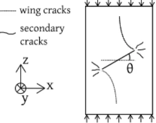
of a unique flaw (see Fig. 1). This corresponds to mode I+II loading, and 18
pioneering experiments based on this configuration were undertaken mainly on 19
˚
model materials (gypsum, PMMA, glass, etc...) as presented in [1, 2, 3]. These 20
authors observed what is now classicaly denoted as wing or primary cracks and 21 secondary cracks. 22 θ x z y wing cracks secondary cracks
Figure 1: Compression of a pre-cracked sample.
Wing cracks are localized crack patterns propagating along the most com-23
pressive stress direction from the flaw tips. Secondary cracks are located near 24
the flaw tips, forming after the wing cracks and extending in a more restrained 25
and diffuse manner compared to the latters (see e.g. [2, 4]). Generally, a tensile 26
nature is associated to wing cracks, whereas secondary cracks, sometimes de-27
noted as shear cracks, would arise from a shear mechanism [5, 6, 4]. However, 28
some authors may state that these secondary cracks appear through the coales-29
cence of local tensile cracks oriented along a different direction than the wing 30
cracks [7, 8]. 31
Wing and secondary cracks have been observed with distinct shapes in model 32
materials [1, 3, 9, 4], fragile polymers [10, 11, 12] or marble [8]. Their occurrence 33
might be less remarkable in other rock types such as e.g. granite [12]. Nonethe-34
less, wing and secondary cracks are now commonly used by geomechanicians to 35
describe crack propagation and coalescence in rocks [5, 8, 13]. 36
Because of their consequence on the overall behavior of rock and other brit-37
tle materials, numerous models have been proposed to study crack propagation. 38
Analytical derivations have been led, generally at the cost of elasticity hypothe-39
sis [14, 15, 16]. More complex mechanical behaviors can be handled more easily 40
using continuous numerical modellings, such as in [17]. Nevertheless, propagat-41
ing cracks are difficult to describe with continuous numerical modellings; though 42
this can still be done using meshless methods such as XFEM [18]. 43
44
On the other hand, discrete multi-scale models describe efficiently by nature 45
both crack propagation and complex mechanical behavior. The inherent discrete 46
structure of rock involving a cohesive assembly of minerals as in granite, or 47
grains as in sandstone, is one reason to use such discrete models. Furthermore, 48
the Discrete Element Method for instance (DEM, [19]) has proven to be an 49
efficient modelling approach for crack propagation analysis in brittle materials 50
[20, 21, 22, 23, 24], including rock [25]. For this reason, many recent works 51
rely on the DEM to study damage in rock, in order to reproduce experimental 52
results such as accoustic emissions [26, 27] or constitutive behavior [28, 29]. 53
Crack propagation from an open flaw has been studied with DEM, mainly in 54
2D [30, 12, 31]. In the regular lattice model of [30], wing cracks could be 55
generated, with a limited kink. The damage patterns obtained in [12, 31] were 56
less marked: this may arise from the heterogeneous strength parameters in these 57
models, which might be related to the differences obtained experimentally for 58
different materials. 59
One can note that less studies consider crack propagation from closed flaws. 60
Experimentally, it is difficult to generate closed flaws with controlled properties 61
[9], but some results suggest similar crack propagation patterns from open or 62
closed flaws [9, 6, 4]. Closed flaws were simulated in DEM in 2D [32] and in 63
3D [33], with, however, contradictory conclusions regarding the numerical re-64
quirements for wing crack simulations. This will be discussed in section 5.2, 65
considering different approaches to model closed flaws. As it will be empha-66
sized in the paper, modelling closed flaws with DEM may be biaised due to the 67
spherical shape of the discrete particles if the formulation is not upgraded. 68
69
Aiming to study crack propagation in rock with various flaw properties, our 70
objective is twofold. First, we aim to propose an approach that is valid for either 71
open or closed planar flaws. Second, we seek to get micro-mechanical insights 72
on the damage mechanisms associated to wing and secondary cracks. 73
First, the DEM model used to simulate the rock matrix is presented in sec-74
tion 2. The model relies on previous developments [29], and its limitations 75
are discussed. The micro-mechanical tools are also introduced. Section 3 dis-76
cusses how closed flaws are simulated in the DEM model. In section 4, crack 77
propagation is studied considering the case of open flaws, comparing the numer-78
ical results with available experimental ones. Section 5 presents mechanically 79
consistent simulations of crack propagation from closed flaws with different me-80
chanical properties. Finally, section 6 provides micro-mechanical insights into 81
wing and shear cracks propagation. 82
All simulations are performed with the open-source code Yade [34, 35], and 83
the geomechanics sign convention is used throughout the whole paper, consid-84
ering compressive stresses and strains as positive. 85
2. Rock matrix modeling 86
2.1. Model formulation
87
Rock matrix is simulated using a packing of bonded spherical discrete ele-88
ments (also denoted particles in the present article). The core of the model, 89
previously presented in [29], is to some extent similar to other DEM models for 90
rock [25, 28]. A major difference relies in the consideration, here, of near neigh-91
bour interactions through a controlled interaction range. Indeed, interparticle 92
bonds are created between each pair of particles A and B for which equation 93
(1) is fullfilled: 94
DAB0 ď γintpRA` RBq (1)
In equation (1), RA and RB are the radii of the two particles, DAB0 the initial
95
distance between the two centro¨ıds of A and B, and γint ě 1 a parameter of
96
the model. With such controlled near neighbour interactions, first proposed 97
in [36], the average number of bonds per particle, N , can be predefined. This 98
feature is motivated by the inadequate UCS/UTS ratios provided by classical 99
DEM using spherical particles [25, 37], UCS (resp. UTS) being the uniaxial 100
compressive (resp. tensile) strength. The mean contact number N being related 101
to the UCS/UTS ratio [29], the γint-parameter provides the possibility to define
102
precisely N and to simulate various rock types. 103
As an alternative, the use of clumps (rigid aggregates) of spheres has been 104
proposed as a solution for 2D simulations [38], but the same method might 105
lead to less significant improvements in 3D [39]. Other solutions would be to 106
adapt the contact laws of the parallel bond model of [25], introducing up to 10 107
parameters [39], or using the so-called flat joint contact model which has been 108
developped up to now for the 2D case [40]. The use of a controlled interaction 109
range with one scalar parameter γint provides an efficient approach simple to
110
formulate. 111
The behavior of the medium is defined through normal and tangential in-112
teraction forces acting between interacting particles. Within DEM, interac-113
tion forces are classically computed from the relative displacement between 114
particles. DAB being the current value of the distance between the two
cen-115
tro¨ıds, the normal force Fn is computed from the normal relative displacement
116
un “ D0AB´ DAB (un increases when spheres get closer to each other). Both
117
repulsive (compressive), and cohesive (tensile), normal forces are considered. In 118
tension, normal forces can develop up to a threshold Fmax
n such that:
119
Fn“ knun while knuną ´Fnmax; Fn “ 0 otherwise (2)
with Fmax
n “ t Aint ą 0 computed from the tensile strength t (in Pa) and
120
Aint “ π minpRA, RBq2, a surface related to the interacting particles. The
121
normal stiffness kn is computed as a function of the particles radii and Y , a
122
parameter of the model expressed in Pa: 123
kn“
2 Y RARB
RA` RB
(3) Equation (3) expresses the normal stiffness as the one of two spring series with 124
stiffnesses Y 2RA{B, that can be interpreted as the stiffnesses of two elastic
125
particles. In the end, Y is related, though different, with the bulk modulus of 126
the numerical sample. 127
The tangential local stiffness ktis deduced from the second elastic parameter
128
of the model, P (dimensionless) such as: 129
The tangential force ~Ft is linearly incremented using kt and the incremental
130
relative tangential displacement ~∆ut. Tangential forces can increase in norm up
131
to a cohesive-frictionnal threshold Fmax
t computed from the local friction angle
132
ϕand the cohesion parameter c (in Pa): Fmax
t “ c Aint` Fn tanpϕq .
133
Interparticle bonds may fail through tension or shear when the normal force 134
or the tangential force reach respectively´Fmax
n or Ftmax. Then, the interaction
135
disappears in the tensile regime if Fn ă 0, or keeps going in a compressive regime
136
if Fně 0. For the latter case, the behavior becomes purely frictionnal: t and c
137
are set to zero. From this point, Fn ě 0 (Fnmax “ 0) and Ftmax“ Fn tanpϕq.
138
The same purely frictional behavior rules the interactions appearing during the 139
simulation when spheres come in strict geometrical contact (i.e. γint“ 1).
140
An explicit time-domain integration scheme is used to solve the equations 141
of motion. The discrete elements are thus translated and rotated according to 142
the interaction forces and their resulting torques using Newton’s second law. 143
Because of the dynamic formulation of the method, damping is used in the 144
model to dissipate kinetic energy, as described in the following section. 145
Table 1 presents the retained parameter values. The resulting UCS, UTS 146
and Young’s modulus are respectively 70 GPa, 6 GPa and 55 GPa (see next 147
sections), which corresponds to a Carboniferous Limestone [41]. A detailed 148
presentation of the calibration process can be found in [33, 29]. Note however 149
that a complete quantitative description of this specific rock is out of the scope 150
of our qualitative analysis.
N Y (GPa) P ϕ(0) c (MPa) t (MPa)
12 50 1/3 18 45 4.5
Table 1: Considered model parameters for the intact rock.
151
2.2. Numerical damping
152
A local non-viscous damping [42] is used, introducing a damping force ~Fd
153
in Newton’s second law such that: 154 ~ Fd“ ´α sign ˆ Σ ~Fptq¨ ˆ ~vptq`dt2~aptq ˙˙ Σ ~Fptq (5)
~
Fd depends on the damping parameter α P r0; 1s, α “ 0 corresponding to an
155
undamped system. This damping method facilitates quasi-static simulations, 156
by dissipating kinetic energy in the model. Note that energy dissipation is also 157
included in the model through sliding and brittle failure processes. Few authors 158
present damping as an indirect modelling of other physical energy dissipation 159
sources [26, 25]. In this case, α should be considered as a model parameter 160
that would require experimental measurements such as seismic quality factor 161
for calibration. However, retained α values are in the end not consistent with 162
this approach (see e.g. [25]). 163
Here, damping is considered only as a convenient numerical treatment that 164
reduces computational costs, since it allows quasi-static conditions with higher 165
loading rates. Then, its possible influence on the results is assessed by simulating 166
uniaxial compression tests for different values of α, with the parameters of Table 167
1. 168
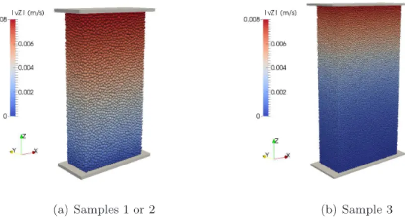
Uniaxial tests simulations consist in the loading of a parallellepipedic sample 169
of spherical particles between two rigid platens (see the Fig. 3). Deformation of 170
the sample is caused by the movement of one platen toward the other at a con-171
stant speed. The platens are frictionless to favour a homogeneous deformation 172
inside the sample. Details about the simulation procedure and the influence of 173
the platen friction angle were given in [29]. Here, stresses deduced from the 174
force acting on the moving platen, and the one deduced from Love-Weber ho-175
mogeneization formula [43, 44] are equal, confirming an acceptable level of the 176
homogeneity and quasi-staticity within the model. 177
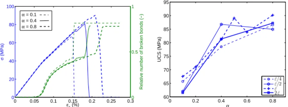
As shown in Fig. 2, the pre-peak behavior is not affected by damping, but 178
the UCS increases (up to 30 % here) according to α. Failure occurs along with a 179
brutal increase in the number of broken bonds (Fig. 2). At the stress peak, the 180
perturbations induced by the rupture of one interaction trigger a chain reaction 181
leading to the failure of a set of bonds that will consequently bisect the sample 182
[26]. Such chain reaction is inhibited by the damping, thus delaying failure and 183
increasing the stress that may be reached (Fig. 2). Similar trends were reported 184
in [26, 45, 28]. Note that different simulations run with different loading rates 185
show the same trends, which means that quasi-staticity is ensured up to the 186
peak in every case. 187 0 0.05 0.1 0.15 0.2 0.25 0.3 0 20 40 60 80 100 σ (MPa) ε1 (%) 0 0.5 1
Relative number of broken bonds (−)
α = 0.1
α = 0.4
α = 0.8
(a) Reference loading rate case. The number of broken bonds is relative to the initial num-ber of bonds 0 0.2 0.4 0.6 0.8 60 65 70 75 80 85 90 95 α UCS (MPa) ˙ε/4 ˙ε/2 ˙ε 2 ˙ε
(b) UCS for different loading rates around the reference 9ε « 7.4 ˆ 10´4s´1
Figure 2: Damping influence for uniaxial compression test simulation.
The significant UCS variations reveal an inherent problem of the model 188
formulation, due to the introduced damping and the brittleness of the contact 189
law; even though such model is quite classical for rock simulations [26, 25, 45, 190
28, 29]. As such, a constant low-level damping is used throughout this study: 191
α “ 0.2, which is rather limited compared to other works: α “ 0.7 in [25],
192
α“ 0.4 in [29]. Doing so, we approach the behavior of an undamped model,
193
keeping reasonnable computational costs. 194
2.3. Discrete element size influence
195
As, e.g. for computational cost reasons, the particles used in the simulations 196
do not correspond in number and in size to real physical entities, the influence of 197
particle size on the results has to be considered. Uniaxial compressive tests were 198
performed on three different numerical samples (Table 2) using the parameters 199
presented in Table 1. 200
Samples 1 and 2 contain around 21000 particles with a mean diameter D«
201
22 cm‹. However, they do not involve the same packing due to the random
202
Designation Number of elements Mean diameter (m)‹
Sample 1 20689 0.215
Sample 2 20689 0.215
Sample 3 124137 0.118
Table 2: Samples used for studying size dependency. For all samples, Lx« 5.4 m, Ly« 2.4 m,
Lz « 10.8 m, and a uniform distribution of radii is used with Dmax{Dmin « 1.86. The
px, y, zq framework is depicted in Fig. 3, z being the loading direction.
generation process. Sample 3 contains around 124000 particles, with a mean 203
diameter D1 « 12 cm. In accordance with Table 1, the mean coordination
204
number N is set to 12 in every case, which requires slight changes in parameter 205
γint among the different samples. The three samples contain enough particles
206
(ą 10000) to ensure a representative behavior and to focus on the influence of
207
the mean diameter only.
(a) Samples 1 or 2 (b) Sample 3 Figure 3: Different samples loaded in uniaxial compression.
208
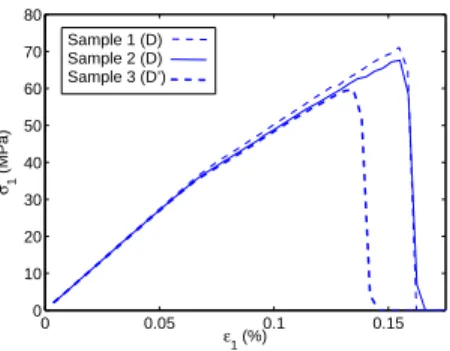
As shown in Fig. 4, the same macroscopic elastic stiffness is obtained what-209
ever the mean diameter. This results from the introduction of the radii of the 210
particles in equation (3). Concerning the plastic behavior, both samples with 211
the same mean diameter D exhibit a similar strength with a difference of about 212
5% for the stress peak. However, greater differences appear for the third sample 213
that involves smaller particles with mean diameter D1 ă D. The stress peak
214
0 0.05 0.1 0.15 0 10 20 30 40 50 60 70 80 ε1 (%) σ1 (MPa) Sample 1 (D) Sample 2 (D) Sample 3 (D’)
Figure 4: Uniaxial compressive test for different samples (D’« D/2) with same parameters.
is here reduced by about 13% when the mean diameter decreases. This is re-215
lated to the elastic-brittle interaction laws that induce an influence of the mean 216
diameter on the fracture toughness, explained as follows. 217
For illustrative purposes, let us consider a monodisperse packing of bonded 218
spheres of diameter D (Fig. 5). A crack of surface Ac exists in the packing, due
219
to previous bond breakages (Fig. 5(a)). The rupture of another bond induces 220
a growth of the crack surface by dAc (Fig. 5(b)). Under pure tensile loading
221
(no shear forces), the energy released during this bond breakage is equal to 222 E“ 1{2 pFmax n q 2 {kn. 223 Ac
(a) Before crack prop-agation Ac dAc cohesive interaction broken (former cohesive) int.
(b) After crack propagation
Figure 5: Crack propagation in a DEM model.
Within our model, the critical fracture energy [46] Gc “ E{dAc9E{D2
de-224
pends finally on the model parameters t, Y and on the sphere diameter D such 225 that: 226 Gc 9 t 2 YD (6)
Thus, for what concerns localized failure mechanisms, the discrete model suffers 227
from a size dependency: the critical surface energy is proportional to the mean 228
diameter D, or, equivalently, the fracture toughness is proportional to ?D.
229
Using a different approach, the same conclusion has been drawn in [25]. If the 230
toughness was to be set without any particle size-dependency, the interaction 231
law should be modified, introducing another parameter, as suggested in [21]. 232
Nevertheless, the following sections will show that the model still has advantages 233
to study qualitatively crack propagation. Quantitative comparisons can also be 234
led as long as the same discretization size is kept. 235
2.4. Micro-mechanical insight
236
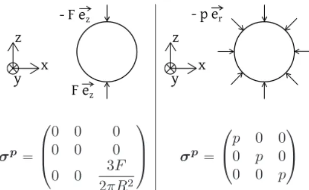
For any material system, it is possible to define a symmetric tensor that 237
expresses the power of internal forces, that is thus related to a stress tensor 238
[47, 48, 49]. For a system made up of one particle p at equilibrium under 239
interaction forces related to several contact points c, the symmetric internal 240
moment tensor Mp [48, 49] can be used, expressed by:
241
Mp “ÿ
c ~
xcb ~fc (7)
with ~xc the position of the interaction points (from the center of the particle
242
p) where the interaction forces ~fc apply. A stress tensor at the particle scale, 243
denoted as particle stress tensor, is then derived as: 244
σp“ ´1{VpMp (8)
with Vp the volume of the particle (the minus sign is set to obey the
geome-245
chanical sign convention). For illustration purpose, Table 3 gives two examples 246
of σp values.
247
Considering a set S of particles, the related internal moment tensor MS is
248
the sum of the internal moment tensors of each particle included in S. If S 249
contains enough particles so that it can be considered as a REV, a direct link 250
appears between MS and the Cauchy stress tensor [49], which may justify the
251
definition of σp. However, one particle can not constitute a REV for a DEM
252
assembly, then σp is a local value that relates to the mechanical state of the
253
assembly in a qualitative manner only. 254
x z y - F ez F ez x z y - p er σp“ ¨ ˚ ˝ 0 0 0 0 0 0 0 0 3F 2πR2 ˛ ‹ ‚ σp“ ¨ ˝ p 0 0 0 p 0 0 0 p ˛ ‚
Table 3: σpfor two given micro-mechanical loadings: opposite forces, or uniform pressure.
The field of major (most compressive) principal stresses σIpcomputed during
255
the pseudo elastic phase (pre-peak) of a uniaxial compression test is presented 256
in Fig. 6 (details about such representations are given in Appendix A). Firstly, 257
it can be observed that the principal directions of σpI, at the particle scale,
258
conform to the principal stress direction imposed at the macroscopic scale (Fig. 259
6(a)). Secondly, the major principal particle stresses are here in a certain extent
(a) Direction of major principal stress (most compressive)
|σIp − <σ I p>| / <σ I p> 0.05 0.1 0.15 0.2 0.25 0.3 0.35 0.4 0.45 0.5
(b) Heterogeneity of the ma-jor principal stress
Figure 6: Micro-mechanical state of the DEM model in the pseudo-elastic phase of an uniaxial compression test.
260
uniform, as might be expected from such homogeneous test (Fig. 6(b)). Indeed, 261
σIp values differ from the mean ă σIp ą by 50% maximum. Finally, the data
set shows that both other principal stresses are similar and negligible compared 263
with σIp, for all particles. 264
These results support the use of σpas a qualitative micro-mechanical insight
265
to evaluate the stress distribution at the particle scale. The method will thus 266
be used in section 6 to analyze crack propagation. 267
3. Rock discontinuities modeling 268
Pre-existing discontinuity surfaces are handled in a specific manner inside 269
the rock model. A smooth-joint model (SJM, [50]) is applied to the joint inter-270
actionsthat concern particles located on both sides of any discontinuity surface.
271
Using the SJM, the normal and tangential vectors of the interaction are rotated 272
and defined according to the surface of interest, rather than upon the contact 273
geometry of the spherical particles. The elastic-plastic constitutive relations 274
presented in section 2 hold for joint interactions, with adequate expressions of 275
normal and tangential relative displacements. Namely, for such interactions 276
un “ p ~AB 0
´ ~ABq.~n with ~n the normal vector to the discontinuity surface, from 277
center A to center B. ~n is thus different from ~AB{|| ~AB||. The plastic behavior, 278
defined according to a friction angle φ and a dilatancy angle ψ, is independent 279
of the discretization of the model [33]. In order to get rid of the size dependency 280
also in the elastic domain, the elastic local stiffnesses kn and ktare given by:
281
kn “ Knj Aint kt“ Ktj Aint
(9)
with the interface parameters Kj
n and K
j
t expressed in Pa/m.
282
Compression and shear tests were conducted on a numerical rock joint to 283
confirm the discretization-independence. A planar joint is defined in a par-284
allelepipedic sample by assigning a SJM to all interactions located across the 285
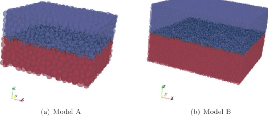
corresponding surface (Fig. 7). The particles lying on each side of the surface 286
are clumped together, in order to form two rigid blocks on each side of the rock 287
joint. With this method, different from the ones used in [51, 33], the local pa-288
rameters of the joint can be tested directly without any influence of the matrix 289
parameters (the latter is considered as a rigid body). The joint normal and
(a) Model A (b) Model B
Figure 7: Particles (spheres) and joint interactions (lines) of the rock joint discrete models. Model A describes the joint surface with particles of mean diameter D « 0.63. Model B involves particles with D« 0.29.
290
tangential stresses, denoted σ and τ , are directly deduced from the interact-291
ing forces occurring between the clumps. The normal and tangential relative 292
displacements are denoted u and γ respectively. 293
The rock joint is first normally loaded through a compression along the ~z 294
axis (Fig. 7): du“ cst ą 0; dγ “ 0. The compression is performed at constant
295
speed up to σ« 1 MPa. A second phase of constant normal displacement (CND)
296
shear modepdu “ 0; dγ “ cst ą 0q is then applied along the ~x axis, Fig. 7. The
297
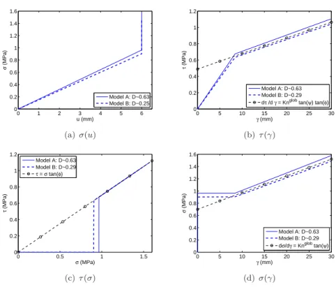
constitutive behavior of the model is presented in Fig. 8. It corresponds to an 298
elastic-plastic rock joint with two elastic stiffnessespKglob
n ; K
glob
t q and a plastic
299
behavior with constant yield surface τ “ σ tanpφq and flow rule dup{|dγp| “
300
´ tanpψq. The plastic behavior is obtained during shear displacement from 301
pγ, τq « p9 mm, 0.7 MPaq. Appendix B derives the equations of the curves that 302
are plotted along the model’s response in Fig. 8. 303
As shown in Fig. 8(a) and 8(b), the macroscopic elastic stiffnesses Kglob
n and
304
Ktglobcan be considered to be unaffected by the mean diameter of the numerical
305
sample. They depend on the micro-parameters Kj
n and K
j
t, and on the ratio
306
between the sum of all interaction surfaces Aint and the apparent joint surface;
307
which is directly related to the density of the packing. This dependence on the 308
0 1 2 3 4 5 6 0 0.2 0.4 0.6 0.8 1 1.2 1.4 1.6 u (mm) σ (MPa) Model A: D~0.63 Model B: D~0.25 (a) σpuq 0 5 10 15 20 25 30 0 0.2 0.4 0.6 0.8 1 1.2 γ (mm) τ (MPa) Model A: D~0.63 Model B: D~0.29
dτ /d γ = Knglob tan(ψ) tan(φ)
(b) τpγq 0 0.5 1 1.5 0 0.2 0.4 0.6 0.8 1 1.2 σ (MPa) τ (MPa) Model A: D~0.63 Model B: D~0.29 τ = σ tan(φ) (c) τpσq 0 5 10 15 20 25 30 0 0.2 0.4 0.6 0.8 1 1.2 1.4 1.6 γ (mm) σ (MPa) Model A: D~0.63 Model B: D~0.29 dσ/dγ = Knglob tan(ψ) (d) σpγq
Figure 8: Behavior of two rock joint discrete models involving two different samples. All computations are made with Kjn“ 50 MPa/m, Ktj“ K
j
packing density induces a difference between Kj
n and Knglob such that: Knglob«
309
155˘5 MPa/m while Kj
n“ 50 MPa/m. However, equality between other
micro-310
parameters and induced macro-properties is obtained: Ktglob{Knglob“ K j
t{Knj “
311
0.5, and the macro-plastic parameters φ and ψ are the same as those introduced 312
at the interaction scale. This direct correspondance is remarkable in DEM and 313
has to be pointed out. 314
4. Crack propagation from an open flaw 315
DEM simulations of open pre-existing cracks is straightforward: the particles 316
are simply removed at the flaw location. Here, the three samples presented in 317
Table 2 are subjected to uniaxial compression, including a flaw located at their 318
center and persistent through the ~y direction. The flaw length, in the p~x, ~zq
319
plane, is 20% of Lz.
320
4.1. Strength of pre-cracked samples with open flaws
321
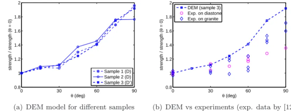
The uniaxial compressive tests performed on samples with an open flaw show 322
a continuous increase of the strength with the flaw orientation θ (Fig. 9(a)). 323
Such trend is in qualitative agreement with experimental results obtained in [12] 324
(Fig. 9(b)), and with discrete modelings performed by [12, 31]. One can note 325
moreover that this result is not affected by the discretization of the model, i.e. 326
the numerical assembly. 327 0 30 60 90 0.8 1 1.2 1.4 1.6 1.8 2 θ (deg) strength / strength ( θ = 0) Sample 1 (D) Sample 2 (D) Sample 3 (D’)
(a) DEM model for different samples
0 30 60 90 0.8 1 1.2 1.4 1.6 1.8 2 θ (deg) strength / strength ( θ = 0) DEM (sample 3) Exp. on diastone Exp. on granite
(b) DEM vs experiments (exp. data by [12]) Figure 9: Strength of pre-cracked samples (open cracks) with different crack inclinations.
Quantitatively, different values of the U CSpθ “ 900q{UCSp00q ratio may be
328
obtained: around 2 in the present numerical study, 1.2 in [31] and 1.3 to 1.7 in 329
[12]. This difference may be related to the geometry of the open flaw that is 330
different in every case. 331
4.2. Crack propagation patterns from open flaws
332
For flaw inclinations less than 600, distinct wing and secondary cracks can
333
be observed (Fig. 10), resulting from the coalescence of local bond breakages 334
(hereafter denoted as microcracks). This result is in accordance with previous 335
experimental works [2, 4, 8, 13]. The location of the wing crack initiation de-336
pends on the inclination of the pre-existing flaw towards the direction of the 337
major principal stress. For θ“ 00, the crack propagates from the middle of the
338
flaw. For increasing θ-values, the initiation of the wing crack moves along the 339
flaw to finally reach the flaw tip as observed experimentally [8, 4]. 340
For higher inclinations (θě 600here), damage first initiates with a localized
341
pattern, at the flaw tips. Then, secondary cracks appear nearby and prevent 342
localization, so that an unique diffuse pattern develops afterwards (Fig. 10). 343
In our DEM simulations, all microcracks correspond to local tensile bond 344
failures. This is directly related to the interparticle bond strength properties 345
which were calibrated to ensure the macroscopic behavior to be representative 346
of a brittle rock (carboniferous limestone), with the local tensile strength that is 347
significantly smaller than the local shear strength. Such a result would support 348
the idea that the secondary cracks, or shear cracks, appear in fact through the 349
coalescence of local tensile cracks oriented along another direction than the wing 350
cracks [7, 8]. This point will be discussed in section 6.1. 351
Note that the obtained crack propagation patterns do not depend on the 352
discrete element size (Fig. 11). 353
5. Crack propagation from a closed flaw 354
Closed flaws can be simulated in DEM by removing the cohesive feature of 355
all interactions located along the flaw surface as proposed by [52, 25, 32]. For 356
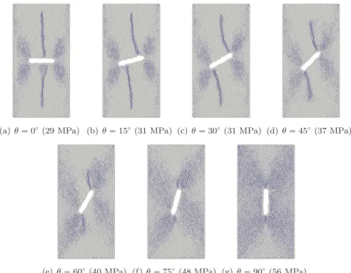
(a) θ“ 00 (29 MPa) (b) θ“ 150(31 MPa) (c) θ“ 300 (31 MPa) (d) θ“ 450 (37 MPa)
(e) θ“ 600(40 MPa) (f) θ“ 750(48 MPa) (g) θ“ 900(56 MPa)
Figure 10: Crack propagation patterns from open flaws: blue dots correspond to broken interparticle bonds locations. For σ values all in the range [0.64 UCS; 0.71 UCS]. Strengths for each case are indicated in parenthesis in corresponding labels.
(a) θ“ 00, sample 1: D (29 MPa) (b) θ“ 00, sample 3: D’ă D (25 MPa) (c) θ“ 300, sample 1: D (31 MPa) (d) θ “ 300, sample 3: D’ă D (28 MPa) Figure 11: Crack propagation pattern from open flaws, obtained for different model discretiza-tions. At σ“ 21 ˘ 1 MPa (peak stresses of each case are indicated in label).
such approach, due to the spherical geometry of the particles, the influence of 357
the discretization of the model is questionable since the simulated flaw surface 358
present a roughness that depends on the size distribution of the particles located 359
on each side of the discontinuity surface. To discuss this point, the use of the 360
SJM is compared with this existing approach. 361
Again, uniaxial compression tests are considered, using the assemblies pre-362
sented in Table 2. Because the flaw is closed, its mechanical properties have 363
to be determined. All simulations were performed here with Kj
n “ K
j
t “ 5
364
GPa/m, ψ“ 00and different values of φ for the interactions making up the flaw
365
surface. Whatever the approach considered, classic contact model or smooth 366
joint model, all simulations were performed using the same non-cohesive local 367
properties along the flaw interactions. Using the SJM, the contact geometry of 368
these interactions was additionally rotated according to the flaw geometry (see 369
section 3). 370
5.1. Strength of pre-cracked samples with closed flaws
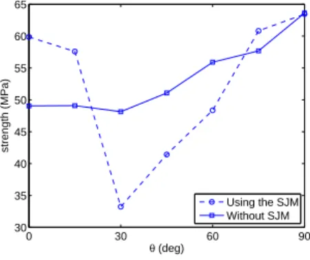
371 0 30 60 90 30 35 40 45 50 55 60 65 θ (deg) strength (MPa) Using the SJM Without SJM
Figure 12: Strength of the pre-cracked sample, considering two closed flaw models (φ“ 180
). Strength of the intact sample was 71 MPa.
As expected, depending on the approach chosen for describing the closed 372
flaw, the responses are different (Fig. 12). For low flaw inclinations (θď 150),
373
the use of the SJM leads to higher strengths, compared to the classical con-374
tact model. With the SJM, the joint interactions are all oriented perpendicular 375
to the flaw and are thus all parallel to the direction of the loading. With-376
out the SJM, the orientations of the interactions along the flaw are randomly 377
distributed, which leads to a lower resistance against the vertical loading. For 378
intermediate inclinations, a drastic decrease of the strength, explained hereafter, 379
is captured using the SJM. Without the SJM, there is a continuous, slight, in-380
crease of the strength according to θ, which is in fact similar to the open flaw 381
case (see previous Fig. 9). In addition, the results obtained without the SJM are 382
significantly affected by the discretization. Indeed, the strength variation with 383
the flaw inclination shows different trends depending on the numerical sample 384 (Fig. 13). 385 0 30 60 90 0.95 1 1.05 1.1 1.15 1.2 1.25 1.3 θ (deg) strength / strength ( θ = 0) Sample 1 (D) Sample 2 (D) Sample 3 (D’)
Figure 13: Strength of the pre-cracked sample for different orientations θ (see Fig. 1): closed flaw (φ“ 180) described removing cohesive interactions across the flaw, without SJM.
On the contrary, using the SJM, very few differences appear using different 386
samples (Fig. 14(a)). Moreover, a mechanically consistent description of the 387
flaw is clearly obtained. In every case, the strength reaches a minimum for 388
an orientation related to the flaw friction angle (Fig. 14(b)). This results 389
from the compressive loading, that imposes mainly vertical chains of contact 390
forces between discrete elements (see e.g [53]). And, for θą φ, sliding occurs
391
for all joint interactions carrying vertical contact forces. Whereas there is no 392
restriction for vertical contact forces along the flaw while θď φ. For this reason, 393
an approximatively constant strength is obtained in the inclination range θď φ,
394
while the strength of the sample is significantly reduced for θą φ. This sound
395
result can not be retrieved without the SJM, as shown in Fig. 12 and 13. 396
0 30 60 90 0.5 0.6 0.7 0.8 0.9 1 1.1 1.2 θ (deg) strength / strength ( θ = 0) Sample 1 (D) Sample 2 (D) Sample 3 (D’)
(a) For different samples (φ“ 180
) 0 30 60 90 0.4 0.5 0.6 0.7 0.8 0.9 1 1.1 θ (deg) strength / strength ( θ = 0) φ=0° φ=15° φ=30° φ=45°
(b) For different φ values Figure 14: Strength of the pre-cracked sample using the SJM.
5.2. Crack propagation patterns from closed flaws
397
Simulating closed flaws using the SJM, crack propagation depends on both 398
θ, the flaw inclination, and φ,the flaw friction. 399
The fracturing patterns obtained for φ “ 00 and different values of θ are
400
shown in Fig. 15. No localized wing cracks form from a horizontal closed flaw, 401
as opposed to the open flaw case. For other inclinations the patterns obtained 402
with the closed flaw are in a certain extent similar to the ones obtained for 403
an open flaw. Again, fracturing localizes through wing cracks for intermediate 404
orientations (00ă θ ă 600). However, the wing cracks here always initiates from
405
the tips of the flaw and show a limited kink. Using another numerical method 406
(the displacement discontinuity method), Shen et al. [9] showed an influence of 407
the stiffness of the flaw surface on the curvature of the wing crack: softer flaws 408
were shown to induce more curved wing cracks patterns, the extreme case being 409
the case of an open flaw. 410
Delayed with respect to the straight localized wing cracks, zones of secondary 411
cracks can also be observed. 412
For higher inclinations (θ ą 600 here), fracturing is diffuse throughout the
413
whole sample, almost as if there was no flaw. 414
415
Using other values for the flaw friction angles (φ ą 00) demonstrates that
416
the SJM describes wing cracks propagation for intermediate orientations if and 417
(a) θ“ 00
(55 MPa) (b) θ“ 150
(33 MPa) (c) θ“ 300
(41 MPa) (d) θ“ 450
(41 MPa)
(e) θ“ 600(48 MPa) (f) θ“ 750(58 MPa) (g) θ“ 900(58 MPa)
Figure 15: Closed crack propagation patterns at different inclinations for φ“ 00, using the
SJM. σ values are all in the range [0.6 UCS; 0.7 UCS]. Strengths for each case are indicated in parenthesis with the corresponding labels. The closed flaw appears in black at the middle of the sample.
only if sliding occurs along the flaw (φă θ ă 600). When sliding along the flaw
418
is prevented because φ ě θ, diffuse damage takes place throughout the whole
419
sample and no localized crack develops, as for high inclinations and φ“ 00(Fig.
420
15). Such behavior is in agreement with several experiments [9, 6, 4]. 421
422
When sliding is enabled (φă θ), the fracturing pattern is modified by the
423
frictional strength along the flaw. While increasing φ value, microcracks tend 424
to propagate from the flaw tips in a unique diffuse manner. The two fracturing 425
steps (localized wing cracks followed by diffuse secondary cracks) observed for 426
open flaws or frictionless closed flaws can hardly be distinguished. Fig. 16 427
illustrates the differences observed for θ“ 450with φ“ 0 and 300.
428 (a) εz 0.04 %; σz P [19;20] MPa. Left: φ“ 00 . Right: φ“ 300 . (b) εz0.06 %; σzP [28;29] MPa. Left: φ“ 00 . Right: φ“ 300 .
Figure 16: Flaw friction angle influence on the propagation of a closed flaw (θ“ 450). UCS
is 41 MPa for φ“ 00and 46 MPa for φ“ 300. 429
This influence of the flaw friction angle emphasizes the advantage of using 430
the SJM for simulations of closed crack propagation using spherical discrete 431
elements. Without the SJM, the flaw friction angle can not be precisely assigned 432
to the model, and inadequate fracturing patterns might be obtained. 433
This may explain why here, as in [33], wing cracks are obtained without 434
taking into account a transfer moment law in the DEM; contrary to what has 435
been deduced from a previous discrete study [32] where closed flaws are simu-436
lated without the SJM, by only debonding the elements. Without any friction 437
defined at the contact scale along the flaw, the strength data from this previous 438
study suggest finally a resultant flaw friction angle belonging tor30; 450s (Fig.
439
17). According to our results, such value of the flaw friction angle prevents wing 440 crack to develop. 0 30 60 90 3.2 3.4 3.6 3.8 4 4.2x 10 5 θ (deg) strength (N)
Figure 17: Strengths of pre-cracked samples with closed flaws simulated without the SJM. From data by [32].
441
6. Micromechanical discussion 442
The micro-mechanical quantities presented in section 2.4 are used here to 443
give some insights into crack propagation processes. While the model includes 444
damage through microcracking occurring at contacts, i.e. at an interparticle 445
scale, σp is defined at the particle scale, describing the mechanical state of one
446
given particle surrounded by a set of contacts. However, these micro-mechanical 447
fields represent a valuable meso-scale characterization of the stress state in the 448
medium. 449
6.1. Micro-mechanics of open flaw propagation
450
First of all, using the micro-mechanical values, the DEM model is able to 451
capture the stress concentration caused by the flaw, similarly to any continuous 452
method (e.g. [54]). Let’s consider, for instance, the sample with an open flaw 453
inclined at 300(Fig. 18). The heterogeneity of the major particle stress,
quanti-454
fied by|σpI´ ă σ p
I ą | { ă σ
p
I ą, reaches 3 here (Fig. 18(b)), while it was limited
455
to 0.5 for a homogeneous sample (Fig. 6(b)). The presence of the pre-existing 456
flaw severely disturbs the stress distribution inside the material, with high stress 457
concentrations at its tips and reduced stresses in some shielded areas. As shown 458
in Fig. 10, fracturing initiates in the zones corresponding to these extreme stress 459
values, with shear and wing cracks being different in nature.
(a) Major principal stress (most compressive) map
(b) Variations of the major principal stress
(c) Directions of the major prin-cipal stress around the flaw Figure 18: Micro-mechanical stress for a sample with an open flaw (θ“ 300
) under compression (σ« 22 MPa). See Fig. 10 for corresponding crack pattern.
460
On one hand, shear – or secondary – cracks tend to develop in highly com-461
pressed zones, i.e. zones sustaining high deviatoric stresses for such unconfined 462
loading. Figure 19 depicts a direct comparison between the crack pattern and 463
the particles sustaining the greatest deviatoric stresses spthroughout the model,
464
emphasizing the shear nature of the secondary cracks. On the other hand, wing 465
cracks are clearly not related to shear local stresses. 466
As a matter of fact, wing cracks develop where particles sustain a tensile 467
loading. To emphasize this point, we now consider the quantity pσpIII` σ
p
Iq
468
for each particle. Negative values correspond to particles with the most tensile 469
stress σpIII negative (i.e. corresponding actually to tension) and greater in
470
absolute value than the most compressive stress σIp. As seen in Fig. 20, there
471
is a very good agreement between the wing crack locations and the particles 472
predominantly loaded in tension. First, before fracturing initiates, a lens of 473
(a) σ« 14 MPa (maxp||sp||q « 64 MPa)
(b) σ« 22 MPa (maxp||sp||q « 100 MPa)
Figure 19: Crack patterns and particles with||sp|| ą 0.35 maxp||sp||q for a sample with an
open flaw (θ“ 300, UCS = 31 MPa) under compression. The external plattens are visible to
show the extent of the sample.
tensily loaded particles exists around the flaw. Then this lens deforms into 474
a wing pattern along which microcracking occurs. Some stress relaxation is 475
captured after the cracks form: some particles at mid-length of the wing cracks 476
do not obey σpIII` σIp ă 0 anymore and hence are no longer displayed (Fig.
477
20(c) and 20(d)). Finally, it is important to note that secondary cracks are 478
definitely not associated with tensile-loaded particles. 479
In case of high inclination (θ ě 600), the localized damage initiation
evo-480
cated in Section 4.2 is also associated with tensile stresses. However, tensile 481
loaded zones, i.e., wing cracks do not propagate due to the proximity of highly 482
deviatoric loaded zones where secondary cracks arise afterwards (Fig. 21). 483
In addition, the rotation of the local major principal stress directions due to 484
the presence of the flaw is captured in Fig. 18(c). On one hand, wing cracks 485
propagate conforming to the deflected local major principal stress directions 486
confirming here their mode I opening nature. On the other hand, secondary 487
cracks occur in areas with local major principal directions oriented almost ver-488
tically and seem to propagate along no defined direction. 489
(a) σ« 2.5 MPa (b) σ« 9.5 MPa
(c) σ« 14 MPa (d) σ« 22 MPa
Figure 20: Crack patterns and particles with σpIII` σIpă 0 for a sample with an open flaw (θ“ 300, UCS = 31 MPa) under compression. The external plattens are visible to show the
(a) σ« 14 MPa (b) σ« 28 MPa Figure 21: Crack patterns and particles with σpIII` σp
I ă 0 for a sample with an open flaw
(θ“ 750
, UCS = 48 MPa). The external plattens are visible to show the extent of the sample.
6.2. Micro-mechanics of closed flaw propagation
490
In section 5, it has been shown that from closed flaw, crack propagation 491
localizes in wing crack for more specific conditions than from open flaws. When 492
wing cracks occur, a very good correlation can again be found between the 493
wing crack locations and the particles sustaining a mainly tensile state of stress 494
(σpIII` σpI ă 0) as illustrated in Fig. 22. For such cases, with θ ą φ, because
495
sliding occurs along the flaw, tensile stresses develop in the sample above each 496
flaw tip. Again, during wing crack extension, tensile stresses develop at the tip 497
of the wing cracks whereas stress relaxation occurs along the wing crack branch 498
(Fig. 22(c)). Once the wing cracks have reached the sample ends, secondary 499
cracks develop due to the concentration of compressive stresses (Fig. 23). 500
501
For increasing φ values, wing crack propagation is inhibited because sliding 502
along the flaw is reduced, limiting the development of tensile stresses at the tip 503
of the flaw. Indeed, particles sustaining tensile stresses (with σIIIp ` σpI ă 0)
504
are much fewer and are closer to the flaw with φ“ 300 than with φ“ 00, for
505
θ“ 450(Fig. 24). Ultimately, when φą θ, tensile stresses no longer develop in
(a) σ« 3.0 MPa (b) σ« 8.3 MPa
(c) σ« 12 MPa (d) σ« 22 MPa
Figure 22: Crack patterns and particles with σpIII` σIpă 0 for a sample with a frictionless closed flaw (θ“ 300
Figure 23: Micro-mechanical field of major principal stress σpI for a closed flaw with (θ “ 300;φ“ 00) at σ« 22 MPa. The corresponding crack pattern appears in Fig. 22(d)
(a) φ“ 00 (b) φ“ 300
Figure 24: Particles with σpIII` σpI ă 0 for a closed flaw inclined at θ “ 450
with different friction angles. Under εz0.04 %; σzP [19;20] MPa: see the Fig. 16(a) for corresponding crack
the sample and wing cracks cannot grow. In such cases only a negligible amount 507
of particles with σIIIp ` σpI ă 0 is detected.
508
509
Despite the tensile local failure mode of all bond breakages in the model, 510
these micro-mechanical insights support the idea of different damage mecha-511
nisms causing either primary (wing) or secondary (shear) cracks. This empha-512
sizes the advantage of intermediate- (or meso-) scale mechanical measurements, 513
such as the particle stress tensors, for a better characterization of the stress 514
distribution inside the material. 515
7. Conclusion 516
Discrete element modeling of crack propagation in rock under uniaxial com-517
pression has been discussed. The advantages of the model were presented as 518
well as its limitations. It has been shown that, due to the brittle nature of 519
the local interaction laws used, damping and discrete element size influence 520
quantitatively the simulated strength, but not the elastic properties. 521
The model enables to simulate explicitly both open and closed flaws with 522
various associated properties. A special attention has been paid to use an ad-523
equate discrete model for simulating closed flaws. We showed that a realistic 524
elastic-plastic behavior with controlled properties can be obtained using a SJM 525
formulation with as little numerical bias as possible. 526
Strengths and crack propagation patterns were obtained for open and closed 527
flaws with different inclinations and favorably compared with existing experi-528
mental results. The DEM model offers micro-mechanical insights into the differ-529
ent damage mechanisms occurring in brittle materials. In particular, fracturing 530
localizes in the form of wing cracks at locations where tensile stresses develop. 531
Such wing cracks propagate according to the most compressive stress direction. 532
Diffuse zones of secondary cracks are shown to correspond to excess deviatoric 533
compressive stresses. The distribution of deviatoric compressive and tensile lo-534
cal stresses depend on the nature of the flaw (open or closed) as well as on the 535
frictional strength of the flaw (if closed). 536
As such, the flaw friction angle affects crack propagation patterns, as well as 537
the overall strength of the material. Ultimately, when friction increases, wing 538
crack are inhibited and a more diffuse fracturing pattern is observed. That is, 539
crack propagation in the intact material (the matrix) is affected by the flaw 540
properties, and not only by those of the matrix. 541
542
The influence of the flaw properties on crack propagation and on the overall 543
behavior emphasizes the need to use the SJM for DEM simulations of closed 544
flaws, unless discrete particles correspond to physical entities. Such a model 545
could then be applied to study crack coalescence under confined states. It also 546
suggests further improvements of the DEM, by applying SJM to newly created 547
cracks. This would be useful for bonds broken in shear mode, for which contacts 548
still hold after bond breakage. 549
8. APPENDIX A: representations of σp field
550
Micro-mechanical fields such as the one depicted in Fig. 6(b) are illustrated 551
using the following procedure. Because of the reduced thickness of the sample 552
along the y direction (Ly« Lx{2 « Lz{4), plane stresses in the px, zq plane are
553
considered. 554
For a random selection of particles, principal directions of σp can readily
555
be plotted at the location x, z of particles centers (plane projection of the 3D 556
model). 557
A direct illustration of principal stress values for all σppx, y, zq being
im-558
possible, plane representation of another related field is made as follows. The 559
px, zq plane is discretized in a square grid with a cell length dx “ dz “ 0.2 560
m, which is around the mean diameter of particles. All particles whose center 561
lies in one given cell xi, zi are identified. Then, Fig. 6, 18 and 23 rely on a
562
micro-mechanical value of the stress inside each cell, denoted σp
pxi, ziq, that is
563
derived by summing all internal moment tensors of these particles: 564
σppxi, ziq “ ř V
pσp
dx dz Ly
If dx and dz are such that one unique cell would include the whole model, 565
equation (A.1) corresponds to the Love-Weber formula and the macroscopic 566
stress, at the REV scale, is obtained. 567
9. APPENDIX B: elastic-plastic behavior of a rock joint 568
Let us consider an elastic-plastic rock joint. Equation (B.1) rules the elastic 569 behavior: 570 ¨ ˝ dτ dσ ˛ ‚“ ¨ ˝ Ktglob 0 0 Knglob ˛ ‚ ¨ ˝ dγe due ˛ ‚ (B.1)
The (perfectly) plastic behavior occurs on the yield surface τ “ σ tanpφq, and
571
plastic deformation depends on the dilatancy angle ψ through the following flow 572
rule: dup{|dγp| “ ´ tanpψq [55].
573
Being loaded under constant normal displacement shear mode (du“ 0),
un-574
der an initial value of normal stress σ‰ 0, the stress state reaches the plastic
575
limit condition after some elastic deformation. If loading continues, any change 576
in tangential relative displacement is fully plastic from this time: dγ “ dγp.
577
Thus dup“ ´|dγp| tanpψq “ ´|dγ| tanpψq. The total normal relative
displace-578
ment u being constant due to the imposed CND loading, the plastic dilatant 579
behavior of the joint induces changes in the normal stress σ, as derived in equa-580
tion (B.2): 581
du“ due` dup“ 0 ô dσ{Knglob´ |dγ| tanpψq “ 0 ô dσ{|dγ| “ Knglob tanpψq (B.2)
This equation is plotted in Fig. 8(d). For the Mohr plane pσ, τq, the
Mohr-582
Coulomb plastic limit condition imposes dτ “ dσ tanpφq, see Fig. 8(c). By
583
combining this last equation with equation (B.2) the theoretical line for the 584
plastic regime inpγ, τq plane can be deduced, see Fig. 8(b).
585
Acknowledgments 586
The authors thank ANR GeoSMEC (2012-BS06-0016-03) and its principal 587
investigator, Y. Klinger, for funding and stimulating project. 588
References 589
[1] W. F. Brace, E. G. Bombolakis, A note on brittle crack growth in 590
compression, Journal of Geophysical Research 68 (12) (1963) 3709–3713. 591
doi:10.1029/JZ068i012p03709. 592
[2] E. Lajtai, Brittle fracture in compression, International Journal of Fracture 593
10 (4) (1974) 525–536. doi:10.1007/BF00155255. 594
[3] S. Nemat-Nasser, H. Horii, Compression-induced nonplanar crack ex-595
tension with application to splitting, exfoliation, and rockburst, Jour-596
nal of Geophysical Research: Solid Earth 87 (B8) (1982) 6805–6821. 597
doi:10.1029/JB087iB08p06805. 598
[4] C. Park, A. Bobet, Crack coalescence in specimens with open and closed 599
flaws: A comparison, International Journal of Rock Mechanics and Mining 600
Sciences 46 (5) (2009) 819 – 829. doi:10.1016/j.ijrmms.2009.02.006. 601
[5] H. Jiefan, C. Ganglin, Z. Yonghong, W. Ren, An experimental study of 602
the strain field development prior to failure of a marble plate under com-603
pression, Tectonophysics 175 (13) (1990) 269 – 284, earthquake Source 604
Processes. doi:10.1016/0040-1951(90)90142-U. 605
[6] A. Bobet, H. Einstein, Fracture coalescence in rock-type materials un-606
der uniaxial and biaxial compression, International Journal of Rock Me-607
chanics and Mining Sciences 35 (7) (1998) 863 – 888. doi:10.1016/S0148-608
9062(98)00005-9. 609
[7] N. Cho, C. Martin, D. Sego, Development of a shear zone in brittle rock sub-610
jected to direct shear, International Journal of Rock Mechanics and Mining 611
Sciences 45 (8) (2008) 1335 – 1346. doi:10.1016/j.ijrmms.2008.01.019. 612
[8] L. Wong, H. Einstein, Systematic evaluation of cracking behavior in spec-613
imens containing single flaws under uniaxial compression, International 614
Journal of Rock Mechanics and Mining Sciences 46 (2) (2009) 239 – 249. 615
doi:10.1016/j.ijrmms.2008.03.006. 616
[9] B. Shen, O. Stephansson, H. H. Einstein, B. Ghahreman, Coalescence of 617
fractures under shear stresses in experiments, Journal of Geophysical Re-618
search: Solid Earth 100 (B4) (1995) 5975–5990. doi:10.1029/95JB00040. 619
[10] N. Cannon, E. Schulson, T. Smith, H. Frost, Wing cracks and brittle com-620
pressive fracture, Acta Metallurgica et Materialia 38 (10) (1990) 1955 – 621
1962. doi:10.1016/0956-7151(90)90307-3. 622
[11] L. Germanovich, R. Salganik, A. Dyskin, K. Lee, Mechanisms of brittle 623
fracture of rock with pre-existing cracks in compression, pure and applied 624
geophysics 143 (1-3) (1994) 117–149. doi:10.1007/BF00874326. 625
[12] H. Lee, S. Jeon, An experimental and numerical study of fracture co-626
alescence in pre-cracked specimens under uniaxial compression, Inter-627
national Journal of Solids and Structures 48 (6) (2011) 979 – 999. 628
doi:10.1016/j.ijsolstr.2010.12.001. 629
[13] S. P. Morgan, C. A. Johnson, H. H. Einstein, Cracking processes in barre 630
granite: fracture process zones and crack coalescence, International Journal 631
of Fracture 180 (2) (2013) 177–204. doi:10.1007/s10704-013-9810-y. 632
[14] R. Goldstein, R. Salganik, Brittle fracture of solids with arbitrary 633
cracks, International Journal of Fracture 10 (4) (1974) 507–523. 634
doi:10.1007/BF00155254. 635
[15] B. Lauterbach, D. Gross, Crack growth in brittle solids under compres-636
sion, Mechanics of Materials 29 (2) (1998) 81 – 92. doi:10.1016/S0167-637
6636(97)00069-0. 638
[16] J.-B. Leblond, J. Frelat, Crack kinking from an initially closed crack, In-639
ternational Journal of Solids and Structures 37 (11) (2000) 1595 – 1614. 640
doi:10.1016/S0020-7683(98)00334-5. 641
[17] B. Prabel, A. Combescure, A. Gravouil, S. Marie, Level set x-fem non-642
matching meshes: application to dynamic crack propagation in elasticplas-643
tic media, International Journal for Numerical Methods in Engineering 644
69 (8) (2007) 1553–1569. doi:10.1002/nme.1819. 645
[18] N. Mo¨es, J. Dolbow, T. Belytschko, A finite element method for crack 646
growth without remeshing, International Journal for Numerical Meth-647
ods in Engineering 46 (1) (1999) 131–150.
doi:10.1002/(SICI)1097-648
0207(19990910)46:1¡131::AID-NME726¿3.0.CO;2-J. 649
[19] P. Cundall, O. Strack, A discrete numerical model for granular assemblies, 650
G´eotechnique 29 (1979) 47–65. 651
[20] F. V. Donz´e, S. A. Magnier, Formulation of a three-dimensional numerical 652
model of brittle behaviour, Geophys. J. Int. 122 (1995) 790–802. 653
[21] M. Jir´asek, Z. Bazant, Particle model for quasibrittle fracture and applica-654
tion to sea ice, Journal of Engineering Mechanics 121 (9) (1995) 1016–1025. 655
doi:10.1061/(ASCE)0733-9399(1995)121:9(1016). 656
[22] P. Prochzka, Application of discrete element methods to fracture mechanics 657
of rock bursts, Engineering Fracture Mechanics 71 (46) (2004) 601 – 618. 658
doi:10.1016/S0013-7944(03)00029-8. 659
[23] N. M. Azevedo, J. Lemos, J. R. de Almeida, Influence of aggregate de-660
formation and contact behaviour on discrete particle modelling of fracture 661
of concrete, Engineering Fracture Mechanics 75 (6) (2008) 1569 – 1586. 662
doi:10.1016/j.engfracmech.2007.06.008. 663
[24] D. Jauffr`es, X. Liu, C. L. Martin, Tensile strength and tough-664
ness of partially sintered ceramics using discrete element simu-665
lations, Engineering Fracture Mechanics 103 (2013) 132 – 140.
666
doi:10.1016/j.engfracmech.2012.09.031. 667
[25] D. Potyondy, P. Cundall, A bonded-particle model for rock, International 668
Journal of Rock Mechanics and Mining Sciences 41 (8) (2004) 1329 – 1364. 669
doi:10.1016/j.ijrmms.2004.09.011. 670
[26] J. F. Hazzard, R. P. Young, S. C. Maxwell, Micromechanical modeling of 671
cracking and failure in brittle rocks, Journal of Geophysical Research: Solid 672
Earth 105 (B7) (2000) 16683–16697. doi:10.1029/2000JB900085. 673
[27] C. Tang, L. Tham, S. Wang, H. Liu, W. Li, A numerical study of the 674
influence of heterogeneity on the strength characterization of rock un-675
der uniaxial tension, Mechanics of Materials 39 (4) (2007) 326 – 339. 676
doi:10.1016/j.mechmat.2006.05.006. 677
[28] Y. Wang, F. Tonon, Calibration of a discrete element model for intact rock 678
up to its peak strength, International Journal for Numerical and Analytical 679
Methods in Geomechanics 34 (5) (2010) 447–469. doi:10.1002/nag.811. 680
[29] L. Scholt`es, F.-V. Donz´e, A dem model for soft and hard rocks: Role of 681
grain interlocking on strength, Journal of the Mechanics and Physics of 682
Solids 61 (2) (2013) 352 – 369. doi:10.1016/j.jmps.2012.10.005. 683
[30] Y. Wang, X. Yin, F. Ke, M. Xia, K. Peng, Numerical simulation of rock 684
failure and earthquake process on mesoscopic scale, Pure and Applied geo-685
physics 157 (11-12) (2000) 1905–1928. doi:10.1007/PL00001067. 686
[31] X.-P. Zhang, L. N. Y. Wong, Cracking processes in rock-like material con-687
taining a single flaw under uniaxial compression: A numerical study based 688
on parallel bonded-particle model approach, Rock Mechanics and Rock 689
Engineering 45 (5) (2012) 711–737. doi:10.1007/s00603-011-0176-z. 690
[32] Y. Wang, P. Mora, Modeling wing crack extension: Implications for the 691
ingredients of discrete element model, Pure and Applied Geophysics 165 (3-692
4) (2008) 609–620. doi:10.1007/s00024-008-0315-y. 693
[33] L. Scholt`es, F.-V. Donz´e, Modelling progressive failure in fractured 694
rock masses using a 3d discrete element method, International Jour-695
nal of Rock Mechanics and Mining Sciences 52 (2012) 18 – 30. 696
doi:10.1016/j.ijrmms.2012.02.009. 697
[34] V. ˇSmilauer, E. Catalano, B. Chareyre, S. Dorofeenko, J. Duriez, 698
A. Gladky, J. Kozicki, C. Modenese, L. Scholt`es, L. Sibille, J. Str´ansk´y, 699
K. Thoeni, Yade Documentation, 1st Edition, The Yade Project, 2010, 700
http://yade-dem.org. 701
[35] J. Kozicki, F.-V. Donz´e, Applying an open–source software for numerical 702
simulations using finite element or discrete modelling methods, Computer 703
Methods in Applied Mechanics and Engineering 197 (49-50) (2008) 4429– 704
4443. 705
[36] F. Donz´e, J. Bouchez, S. Magnier, Modeling fractures in rock blasting, 706
International Journal of Rock Mechanics and Mining Sciences 34 (8) (1997) 707
1153 – 1163. doi:10.1016/S1365-1609(97)80068-8. 708
[37] H. Huang, B. Lecampion, E. Detournay, Discrete element modeling of 709
tool-rock interaction i: rock cutting, International Journal for Numeri-710
cal and Analytical Methods in Geomechanics 37 (13) (2013) 1913–1929. 711
doi:10.1002/nag.2113. 712
[38] N. Cho, C. Martin, D. Sego, A clumped particle model for rock, Interna-713
tional Journal of Rock Mechanics and Mining Sciences 44 (7) (2007) 997 – 714
1010. doi:10.1016/j.ijrmms.2007.02.002. 715
[39] X. Ding, L. Zhang, A new contact model to improve the simulated ratio 716
of unconfined compressive strength to tensile strength in bonded particle 717
models, International Journal of Rock Mechanics and Mining Sciences 69 718
(2014) 111 – 119. doi:10.1016/j.ijrmms.2014.03.008. 719
[40] D. Potyondy, A flat-jointed bonded-particle material for hard rock, in: 46th 720
US Rock Mechanics/Geomechanics Symposium, ARMA, 2012. 721
[41] T. Waltham, Foundations of Engineering Geology (Third ed.), Taylor & 722
Francis, 2009. 723
[42] P. A. Cundall, Distinct element models of rock and soil structure, in: E. T. 724
Brown (Ed.), Analytical and Computational Methods in Engineering Rock 725
Mechanics, George Allen and Unwin, 1987, pp. 129–163. 726
[43] A. Love, A treatise on the mathematical theory of elasticity, Cambridge 727
University Press, Cambridge, 1927. 728
[44] J. Weber, Recherches concernant les contraintes intergranulaires dans les 729
milieux pulv´erulents, Bulletin de liaison des Ponts et Chauss´ees 20 (1966) 730
1–20. 731
[45] W. L. Lim, G. R. McDowell, Discrete element modelling of railway ballast, 732
Granular Matter 7 (1) (2005) 19–29. doi:10.1007/s10035-004-0189-3. 733
[46] A. A. Griffith, The phenomena of rupture and flow in solids, Philosophical 734
Transactions of the Royal Society of London. Series A, Containing Papers 735
of a Mathematical or Physical Character 221 (1920) 163–198. 736
[47] J. Lemaitre, J.-L. Chaboche, Mechanics of solid materials, Cambridge uni-737
versity press, 1990. 738
[48] J.-J. Moreau, Numerical investigation of shear zones in granular materials, 739
in: D. E. Wolf, P. Grassberger (Eds.), Friction Arching, Contact Dynamics, 740
World Scientific, Balkema, 1997, pp. 233–247. 741
[49] L. Staron, F. Radjai, J.-P. Vilotte, Multi-scale analysis of the stress state 742
in a granular slope in transition to failure, The European Physical Journal 743
E 18 (3) (2005) 311–320. doi:10.1140/epje/e2005-00031-0. 744
[50] D. M. Ivars, M. E. Pierce, C. Darcel, J. Reyes-Montes, D. O. Potyondy, 745
R. P. Young, P. A. Cundall, The synthetic rock mass approach for jointed 746
rock mass modelling, International Journal of Rock Mechanics and Mining 747
Sciences 48 (2) (2011) 219 – 244. doi:10.1016/j.ijrmms.2010.11.014. 748
[51] M. Bahaaddini, G. Sharrock, B. Hebblewhite, Numerical investigation of 749
the effect of joint geometrical parameters on the mechanical properties of 750