OH and HO₂ chemistry in clean marine air during SOAPEX-2

HAL Id: hal-00295446

https://hal.archives-ouvertes.fr/hal-00295446

Submitted on 14 Jun 2004

HAL is a multi-disciplinary open access

archive for the deposit and dissemination of

sci-entific research documents, whether they are

pub-lished or not. The documents may come from

teaching and research institutions in France or

abroad, or from public or private research centers.

L’archive ouverte pluridisciplinaire HAL, est

destinée au dépôt et à la diffusion de documents

scientifiques de niveau recherche, publiés ou non,

émanant des établissements d’enseignement et de

recherche français ou étrangers, des laboratoires

publics ou privés.

SOAPEX-2

R. Sommariva, A.-L. Haggerstone, L. J. Carpenter, N. Carslaw, D. J. Creasey,

D. E. Heard, J. D. Lee, A. C. Lewis, M. J. Pilling, J. Zádor

To cite this version:

R. Sommariva, A.-L. Haggerstone, L. J. Carpenter, N. Carslaw, D. J. Creasey, et al.. OH and HO2

chemistry in clean marine air during SOAPEX-2. Atmospheric Chemistry and Physics, European

Geosciences Union, 2004, 4 (3), pp.839-856. �hal-00295446�

www.atmos-chem-phys.org/acp/4/839/

SRef-ID: 1680-7324/acp/2004-4-839

Chemistry

and Physics

OH and HO

₂

chemistry in clean marine air during SOAPEX-2

R. Sommariva1, A.-L. Haggerstone2, L. J. Carpenter2, N. Carslaw3, D. J. Creasey1,*, D. E. Heard1, J. D. Lee1,**, A. C. Lewis1,**, M. J. Pilling1, and J. Z´ador4

1_{Department of Chemistry, University of Leeds, Leeds, UK} 2_{Department of Chemistry, University of York, York, UK} 3_{Environment Department, University of York, York, UK}

4_{Department of Physical Chemistry, E¨otv¨os University (ELTE), Budapest, Hungary}

*_{Now at Photonic Solutions plc., Gracemount Business Pavilions Unit A2/A3, 40 Captains Rd., Edinburgh, UK} **_{Now at Department of Chemistry, University of York, York, UK}

Received: 17 December 2003 – Published in Atmos. Chem. Phys. Discuss.: 20 January 2004 Revised: 21 May 2004 – Accepted: 2 June 2004 – Published: 14 June 2004

Abstract. Model-measurement comparisons of HOxin

ex-tremely clean air ([NO]<3 ppt) are reported. Measurements were made during the second Southern Ocean Photochem-istry Experiment (SOAPEX-2), held in austral summer 1999 at the Cape Grim Baseline Air Pollution Station in north-western Tasmania, Australia.

The free-radical chemistry was studied using a zero-dimensional box-model based upon the Master Chemical Mechanism (MCM). Two versions of the model were used, with different levels of chemical complexity, to explore the role of hydrocarbons upon free-radical budgets under very clean conditions. The “detailed” model was constrained to measurements of CO, CH4and 17 NMHCs, while the

“sim-ple” model contained only the CO and CH4oxidation

mech-anisms, together with inorganic chemistry. The OH and HO2

(HOx) concentrations predicted by the two models agreed to

within 5–10%.

The model results were compared with the HOx

concen-trations measured by the FAGE (Fluorescence Assay by Gas Expansion) technique during four days of clean Southern Ocean marine boundary layer (MBL) air. The models over-estimated OH concentrations by about 10% on two days and about 20% on the other two days. HO2concentrations were

measured during two of these days and the models overes-timated the measured concentrations by about 40%. Bet-ter agreement with measured HO2 was observed by using

data from several MBL aerosol measurements to estimate the aerosol surface area and by increasing the HO2uptake

coef-ficient to unity. This reduced the modelled HO2overestimate

by ∼40%, with little effect on OH, because of the poor HO2

to OH conversion at the low ambient NOxconcentrations.

Local sensitivity analysis and Morris One-At-A-Time analysis were performed on the “simple” model, and showed

Correspondence to: M. J. Pilling

([email protected])

the importance of reliable measurements of j(O1D) and [HCHO] and of the kinetic parameters that determine the efficiency of O(1D) to OH and HCHO to HO2 conversion.

A 2σ standard deviation of 30–40% for OH and 25–30% for HO2 was estimated for the model calculations using a

Monte Carlo technique coupled with Latin Hypercube Sam-pling (LHS).

1 Introduction

Tropospheric chemistry is strongly dependent on the con-centration of the hydroxyl radical (OH), which reacts very quickly with most trace gases in the atmosphere. Owing to its short boundary layer lifetime (∼1 s), atmospheric concen-trations of OH are highly variable and respond rapidly to changes in concentrations of sources and sinks. Photolysis of ozone, followed by reaction of the resulting excited state oxygen atom with water vapour, is the primary source of the OH radical in the clean troposphere:

O3+hν (λ < 340 nm) → O(1D) + O2 (1)

O(1D) + H2O → OH + OH (2)

About 10% of the O(1D) atoms react through Reaction (2) under typical boundary layer conditions, the rest are deacti-vated to the ground state through collisions with N2and O2,

reforming ozone.

The two major tropospheric sinks of OH are the reactions with CO and CH4. In the clean Southern Hemisphere, CO

and CH4 account for up to 50% each of the total OH loss,

and HO2and CH3O2are the predominant forms of peroxy

radicals formed (Reactions 3, 4, respectively).

CH4+OH + O2→CH3O2+H2O (4)

The OH radical also reacts with non methane hydrocarbons (NMHCs) producing a variety of organic peroxy radicals (RO2). HO2 and CH3O2react with NO producing OH and

CH3O, respectively (Reactions 5, 6).

HO2+NO → OH + NO2 (5)

CH3O2+NO → CH3O + NO2 (6)

However in low NOxconditions peroxy radicals primarily

react through self and cross peroxy-peroxy reactions to form methyl hydrogen peroxide (CH3OOH) and hydrogen

perox-ide (H2O2). HO2 is also recycled back to OH through the

reaction with O3(Reaction 9).

The self reaction of CH3O2also gives CH3O (Reaction 10)

with a branching ratio of 0.33, other pathways leading to the formation of CH3OH and HCHO. The reaction of CH3O

with O2(Reaction 11) is one of the main sources of HCHO

and a very important source of HO2.

HO2+HO2→H2O2+O2 (7)

CH3O2+HO2→CH3OOH + O2 (8)

HO2+O3→OH + 2O2 (9)

CH3O2+CH3O2→2CH3O + O2 (10)

CH3O + O2→HCHO + HO2 (11)

The methyl hydrogen peroxide contributes to OH loss via Reactions (12) and (13) to form CH3O2and HCHO.

CH3OOH + OH → CH3O2 (12)

CH3OOH + OH → HCHO + OH (13)

In studies comparing measured and modelled HOxradical

concentrations, the models usually overestimate [OH] by 20– 50%. A detailed review of the comparisons of modelled and measured concentrations of OH and HO2 can be found in

Heard and Pilling (2003). In particular, several studies have been made in the marine boundary layer.

Eisele et al. (1996) showed that modelled [OH] overesti-mated measurements by a factor of 2 during the MLOPEX-2 campaign. During EASE96 modelled [OH] results were higher than the measurements by ∼40% (Carslaw et al., 1999), while in EASE 97 the model-measurement ratio was on average 2.1 in clean air conditions (Carslaw et al., 2002). During the ALBATROSS campaign, in the Southern At-lantic, Brauers et al. (2001) overestimated OH by 16% on av-erage, while during the WAOSE95 campaign, the agreement between the model and the measurements was ∼50% or bet-ter (Grenfell et al., 1999). In three recent aircraft campaigns in the Pacific Ocean, PEM Tropics A and B and ACE-1, the agreement between modelled and measured OH was 15–20%

in PEM Tropics A and ∼30% in ACE-1 (Chen et al., 2001; Frost et al., 1999) while in PEM Tropics B the model to ob-served ratio was 1.22 on average at the surface (Tan et al., 2001).

There have been fewer measurements of HO2in the MBL.

The agreement between modelled and measured [HO2] is

variable. Some studies show a reasonable agreement with the measurements (within 25%), but generally the models tend to overestimate [HO2] by a factor of 2 or more (Carslaw et al.,

1999, 2002; Kanaya et al., 2000, 2001). In PEM Tropics B Tan et al. (2001) reported a modelled to observed ratio of 1.12 for HO2near the surface.

This paper investigates the radical chemistry of the clean marine boundary layer in the Southern Ocean during the SOAPEX-2 (Southern Ocean Photochemistry Experiment 2) campaign using an observationally constrained box-model based on the Master Chemical Mechanism (Jenkin et al., 1997, 2003; Saunders et al., 2003). The primary aim of SOAPEX-2 was to study free radical chemistry in the re-mote marine boundary layer in the Southern Hemisphere. Sections 2 and 3 of this paper describe the SOAPEX-2 site and the measurements that were made during the campaign. Section 4 describes the models used and Sect. 5 presents the results. Finally, Sect. 6 contains the summary and the con-clusions.

2 Site description

The SOAPEX-2 campaign, involving scientists from the Universities of East Anglia, Leeds and Leicester, from the CSIRO (Commonwealth Scientific and Industrial Research Organization) Melbourne and from the Australian Bureau of Meteorology, took place in austral summer during the pe-riod 18 January to 18 February 1999 at the Cape Grim Base-line Atmospheric Pollution Station (CGBAPS). The station is situated on the north-west tip of Tasmania, Australia, at 40◦410S, 144◦410E, on a cliff-top ∼100 m above sea level and ∼100 m horizontally from the high-water mark. CG-BAPS is part of the World Meteorological Organisation net-work of Global Atmospheric Watch observatories and an ex-tensive program of atmospheric chemistry and meteorologi-cal measurements has been carried out at the site since 1976. Further details about the site are given in Bates et al. (1998). Cape Grim is an ideal location to study free-radical chem-istry in extremely clean conditions (Penkett et al., 1997). It frequently experiences air masses characterized by low con-densation nuclei (CN) and Radon counts (<462 cm−3 _and

<100 mBq m−3, respectively) with the local wind direction in the sector 190◦–280◦. In these “baseline” conditions, air has not passed over land for 5 days or more and is therefore relatively free of anthropogenic influence. Four days, which were characterised by the lowest NOx and NMHCs levels

experienced during the campaign, have been selected to be representative of baseline conditions in the Southern Ocean.

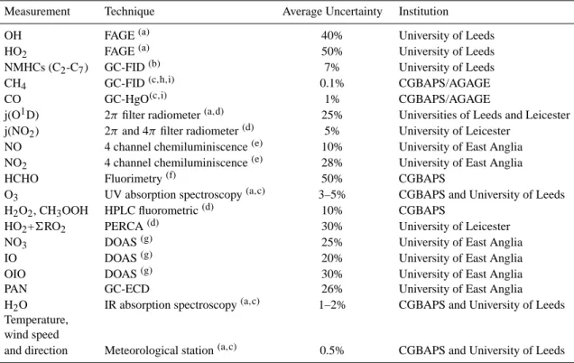
Table 1. Measurements and techniques during SOAPEX-2.

Measurement Technique Average Uncertainty Institution

OH FAGE(a) 40% University of Leeds

HO2 FAGE(a) 50% University of Leeds

NMHCs (C₂-C₇) GC-FID(b) 7% University of Leeds

CH4 GC-FID(c,h,i) 0.1% CGBAPS/AGAGE

CO GC-HgO(c,i) 1% CGBAPS/AGAGE

j(O1D) 2π filter radiometer(a,d) 25% Universities of Leeds and Leicester

j(NO2) 2π and 4π filter radiometer(d) 5% University of Leicester

NO 4 channel chemiluminiscence(e) 10% University of East Anglia

NO2 4 channel chemiluminiscence(e) 28% University of East Anglia

HCHO Fluorimetry(f) 50% CGBAPS

O₃ UV absorption spectroscopy(a,c) 3–5% CGBAPS and University of Leeds

H2O2, CH3OOH HPLC fluorometric(d) 10% CGBAPS

HO2+6RO2 PERCA(d) 30% University of Leicester

NO3 DOAS(g) 25% University of East Anglia

IO DOAS(g) 20% University of East Anglia

OIO DOAS(g) 30% University of East Anglia

PAN GC-ECD 26% University of East Anglia

H2O IR absorption spectroscopy(a,c) 1–2% CGBAPS and University of Leeds

Temperature, wind speed

and direction Meteorological station(a,c) 0.5% CGBAPS and University of Leeds

(a)_{Creasey et al. (2002, 2003).}

(b)_{Lewis et al. (2001).}

(c)_{Bureau of Meteorology and CSIRO Division of Atmospheric Research, Baseline Atmospheric Program reports, Melbourne, Australia,}

1976–1995. (d)_{Monks et al. (1998).} (e)_{Bauguitte (1998, 2000).} (f)_{Ayers et al. (1997).} (g)_{Allan et al. (2001).} (h)_{Cunnold et al. (2002).} (i)_{Prinn et al. (2000).} 3 Experimental

During SOAPEX-2, measurements of the free-radicals OH, HO2, HO2+6RO2, NO3, IO and OIO were supported by

measurements of temperature, wind speed and direction, photolysis rates (j(O1D) and j(NO2)), water vapor, O3,

HCHO, CO, CH4, NO, NO2, peroxyacetyl nitrate (PAN), a

wide range of NMHCs, organic halogens, H2O2, CH3OOH

and condensation nuclei (CN).

Concentrations of OH and HO2were determined, in situ,

using Laser Induced Fluorescence (LIF) at low pressure, (FAGE technique). HO2 cannot be detected directly by

LIF, and was converted to OH by titration with NO di-rectly below the sampling nozzle. The detection limit for the FAGE instrument during SOAPEX-2, determined by cal-ibration in the field, was 1.4×105molecule cm−3 for OH and 5.4×105molecule cm−3for HO2. A description of the

instrument, as set up in previous field campaigns and

dur-ing SOAPEX-2, along with the calibration procedure, is pro-vided elsewhere (Creasey et al., 2002, 2003).

Light non-methane hydrocarbons (NMHCs) were mea-sured using an automated GC-FID system with large volume sample collection onto a Peltier cooled carbon sieve trap fol-lowed by on-line thermal desorption, and separation on an aluminium oxide PLOT capillary column. The system de-ployed at Cape Grim has been described in more detail in a previous paper (Lewis et al., 2001).

The techniques used to measure the other species and pa-rameters are listed in Table 1.

4 Model description

Two versions of a zero-dimensional box-model, containing different chemical schemes, were used to investigate the at-mospheric chemistry of the SOAPEX-2 campaign. Both the

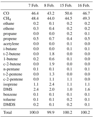
Table 2. Average percentage OH loss due to CO, CH4and NMHCs

during four clean days in SOAPEX-2 (Note that the figures have been rounded up or down to the nearest 0.1%).

7 Feb. 8 Feb. 15 Feb. 16 Feb.

CO 46.4 43.2 50.6 46.7 CH₄ 48.4 44.0 44.5 49.3 ethane 0.2 0.1 0.2 0.2 ethene 0.3 0.4 0.2 0.2 propane 0.0 0.0 0.2 0.1 propene 0.5 0.7 0.4 0.5 acetylene 0.0 0.0 0.1 0.0 i-butane 0.0 0.0 0.1 0.1 t-2-butene 0.0 1.8 0.0 0.0 1-butene 0.2 0.6 0.1 0.0 c-2-butene 0.0 1.9 0.0 0.0 n-pentane 0.1 0.1 0.1 0.1 t-2-pentene 0.0 1.3 0.0 0.0 c-2-pentene 0.0 1.1 1.1 0.0 isoprene 1.1 2.4 1.1 1.1 DMS 2.4 2.0 1.0 1.6 benzene 0.1 0.1 0.1 0.1 toluene 0.1 0.1 0.2 0.1 DMDS 0.2 0.1 0.2 0.1 Total 100.0 99.9 100.2 100.2

“simple” and the “detailed” models were constrained with the observed concentrations of the longer lived species: NOx,

O3, CO, CH4, and HCHO as well as the values of j(O1D),

j(NO2), H2O and temperature. A boundary layer height of

1 km was assumed (Ayers and Galbally, 1994). The “de-tailed” model also contained a full chemical scheme for 17 of the measured NMHCs (see Sect. 4.1). The models were then employed to calculate in situ OH and HO2

concentra-tions, for comparison with each other and the results from the FAGE instrument.

4.1 The “detailed” model

The “detailed” model was constructed as described by Carslaw et al. (1999, 2002). Briefly, measurements of NMHCs, CO and CH4were used to define a reactivity

in-dex with OH, in order to determine which NMHCs, along with CO and CH4, to include in the overall mechanism.

The product of the concentration of each hydrocarbon (and CO) measured on each day during the campaign and its rate coefficient for the reaction with OH was calculated. All NMHCs that are responsible for at least 0.1% of the OH loss due to total hydrocarbons and CO on any day during the campaign are included in the mechanism (Table 2). Re-actions of OH with the secondary species formed in the hy-drocarbon oxidation processes, as well as oxidation by the nitrate radical (NO3) and ozone are also included in the

mechanism. The NMHCs that were found to be important for the SOAPEX-2 campaign were ethane, propane, iso-butane, n-pentane, ethene, propene, trans-2-butene, cis-2-butene, 1-cis-2-butene, trans-2-pentene, cis-2-pentene, acetylene, isoprene, DMS (dimethylsulphide), benzene, toluene and DMDS (dimethyldisulphide). In clean conditions, these 17 NMHCs contributed on average about 5% to the OH loss, while CO and CH4accounted for about 95% (with the

ex-ception of 8 February on which NMHCs accounted for al-most 13% of OH loss). The relative contributions of CO, CH4, DMS, DMDS and NMHCs to OH loss during the four

modelled days are shown in Table 2.

The mechanisms for the NMHCs (except DMS) required to fully characterise OH chemistry were extracted from a re-cently updated version of the Master Chemical Mechanism (MCM 3.0, available at http://mcm.leeds.ac.uk/MCM/). The MCM treats the degradation of 125 volatile organic com-pounds (VOCs) and considers oxidation by OH, NO3, and

O3, as well as the chemistry of the subsequent oxidation

products. These steps continue until CO2 and H2O are

formed as final products of the oxidation. The MCM has been constructed using chemical kinetics data (rate coeffi-cients, branching ratios, reaction products, absorption cross sections and quantum yields) taken from several recent eval-uations and reviews or estimated according to the MCM pro-tocol (Jenkin et al., 1997, 2003; Saunders et al., 2003). The MCM is an explicit mechanism and, as such, does not suffer from the limitations of a lumped scheme or one containing surrogate species to represent the chemistry of many species. The DMS scheme has been taken from the work of Koga and Tanaka (1993), with many of the rate coefficients up-dated as suggested by Jenkin et al. (1996). The reactions of NO3, from the Yin et al. (1990a, b) mechanism, have also

been included.

DMDS was detected at a maximum concentration for clean conditions of 0.38 ppt during SOAPEX-2. The degra-dation of DMDS by both OH and NO3 has been included

according to Jenkin et al. (1996), as well as its photolysis to form two CH3S molecules (Yin et al., 1990a, b). The

oxida-tion products are common to DMS.

Previous work has suggested that Cl atoms may have a bearing on the concentration of many hydrocarbon species, particularly in the marine boundary layer (Keene et al., 1996; Pszenny et al., 1993). The degradation of chlorinated organic species leads ultimately to the release of Cl atoms. Although Cl reacts with O3, it also reacts rapidly with many organic

compounds. Following the protocol for the MCM laid down by Jenkin et al. (1997), we assume that Cl is removed only by reactions with alkanes, as these are less reactive towards OH and are generally present at higher concentrations than other organic species. The precursor species included in the mechanism are CHCl3, CH2Cl2, CH3Cl and C2Cl4, the

con-centrations of which were all determined in this campaign, albeit at low frequency.

The “detailed” model contains 2085 gas-phase reactions, 19 heterogeneous and 116 deposition processes.

4.2 The “simple” model

The “simple” model contained the same inorganic and CO-CH4oxidation schemes as the “detailed” model, taken from

the MCMv3. The model was completed with heterogeneous loss and dry deposition terms, as described in the following section. The chemical mechanism employed in the “simple” model contains 75 gas-phase reactions, 9 heterogeneous and 8 deposition processes and is shown in Table 7.

4.3 Heterogeneous uptake and dry deposition

The models consider a simple parameterization for heteroge-neous loss, where it is assumed that radicals are irreversibly lost upon impacting on aerosol, according to:

khet=

A ¯cγ

4 (14)

where γ is the gas/surface reaction probability, A is the re-active aerosol surface area per unit volume (RASA) (cm−1) and ¯c is the mean molecular speed (cm s−1) (Ravishankara, 1997). There are several species formed in the DMS mecha-nism – DMSO, DMSO2(dimethylsulphone, CH3S(O2)CH3)

and MSA (methane sulfinic acid, CH3S(O)OH) – that are

likely to be readily condensed on existing particles due to their strong hygroscopic nature and low vapour pressure (Koga and Tanaka, 1993).

Heterogeneous uptake on surfaces has also been docu-mented for various free radicals (DeMore et al., 1994). Ta-ble 3 shows values of the gas/surface reaction probabilities (γ ) of the species assumed to undergo loss to aerosol sur-face in the model. Only the species where a reaction prob-ability has been measured at a reasonable boundary layer temperature (i.e. >273 K) and on a suitable surface for the marine boundary layer (NaCl(s) or liquid water) have been

included. Unless stated otherwise, values for uptake onto NaCl(s), the most likely aerosol surface in the MBL (Gras

and Ayers, 1983), have been used. Where reaction proba-bilities are unavailable mass accommodation coefficients (α) have been used instead. The experimental values of the re-action probability are expected to be smaller than or equal to the mass accommodation coefficients because α is just the probability that a molecule is taken up on the particle sur-face, while γ takes into account the uptake, the gas phase diffusion and the reaction with other species in the particle (Ravishankara, 1997).

Large uncertainties exist in the values of these reaction probability coefficients, which tend to vary greatly with both temperature and type of surface.

Dry deposition terms have also been incorporated in the model based on the values of Derwent et al. (1996) except for peroxides (1.1 cm s−1for H2O2and 0.55 cm s−1for

or-ganic peroxides), methyl and ethyl nitrate (1.1 cm s−1) and

Table 3. Reaction probabilities for the heterogeneous loss processes

used in the model.

Species γ Reference

OH 1.25×10−5e(1750/T ) (a) Gratpanche et al. (1996)

HO2 1.40×10−8e(3780/T ) (a) Gratpanche et al. (1996)

CH3O2 4×10−3(at 296 K) Gershenzon et al. (1995)

NO3 4×10−3(at 282–286 K)(b) Allan et al. (1999)

N2O5 0.032 (at 291 K) Behnke et al. (1997)

HNO3 0.014 (at 298 K) Beichert and Pitts (1996)

MSA 0.11 (at 278 K)(c,d) DeBruyn et al. (1994)

SO2 0.11 (at 260–292 K)(c,d) Worsnop et al. (1989)

DMSO 0.08 (at 281 K)(c,d) DeBruyn et al. (1994)

DMSO2 0.08 (at 281 K)(c,d) DeBruyn et al. (1994)

H2O2 0.1 (at 292 K)(c,d) Worsnop et al. (1989)

CH₃OH 0.02 (at 291 K)(c,d) Jayne et al. (1991)

C2H5OH 0.02 (at 291 K)(c,d) Jayne et al. (1991)

1-propanol 0.02 (at 291 K)(c,d) Jayne et al. (1991)

2-propanol 0.02 (at 291 K)(c,d) Jayne et al. (1991)

HOCH2CH2OH 0.04 (at 291 K)(c,d) Jayne et al. (1991)

CH₃C(O)CH₃ 0.013 (at 285 K)(c,d) Duan et al. (1993)

HC(O)OH 0.02 (at 291 K)(c,d) Jayne et al. (1991)

CH3C(O)OH 0.03 (at 291 K)(c,d) Jayne et al. (1991)

(a)_{value at relevant temperature.}

(b)_{estimated by using average of results of Rudich et al. (1996).}

(c)_{measured on liquid water aerosols.}

(d)_{mass accommodation coefficient.}

HCHO (0.33 cm s−1) (Brasseur et al., 1998) and it has been assumed that the dry deposition velocity for CH3CHO and

other aldehydes is the same as that for HCHO.

4.4 Effect of new recommendations for rate coefficients Although the MCMv3.0 was completed quite recently, there have already been some new recommendations for sev-eral of the inorganic rate coefficients, which have been incorporated into both the simple and detailed models. The largest changes concern the pressure-dependent reac-tions of OH with CO and NO2. The rate coefficient of

OH and CO has decreased by 16% (from 2.43×10−13 to 2.05×10−13cm−3molecule−1 s−1 at 298 K), while that of OH and NO2 has increased by 35% (from 8.95×10−12 to

1.21×10−11_cm−3 _molecule−1 _s−1 _{at 298 K) under typical}

boundary layer conditions (Atkinson et al., 2001). Rate co-efficients for the reactions of HO2 with HO2 and O3 have

also been revised following recent laboratory measurements. The difference in [OH] and [HO2] before and after updating

these rate coefficients is small: less than a 10% increase for OH and less than a 2% increase for HO2.

In MCMv3.0 the quenching reaction of O(1D) with N2

has a rate coefficient of 2.58×10−11cm−3molecule−1s−1at 298 K (Atkinson et al., 2001). Recently three groups reported a new rate coefficient of 3.09×10−11cm−3molecule−1s−1

Table 4. Average (11:00–14:00) measurements during the clean

days.

Measurements 7 Feb. 8 Feb. 15 Feb. 16 Feb.

H2O/molecule cm−3 2.5×1017 3.3×1017 3.4×1017 3.7×1017 j(O1D)/s−1 2.2×10−5 2.9×10−5 3.5×10−5 2.8×10−5 j(NO2)/s−1 8.9×10−3 9.1×10−3 9.7×10−3 8.3×10−3 O3/ppb 14.9 13.5 18.5 17.6 NO/ppt 0.8 3.7 1.5 2.4 NO2/ppt 7.5 8.8 12.1 14.8 CH4/ppb 1687 1694 1685 1686 CO/ppb 40.7 45.6 39.9 39.6 HCHO/ppt 352 217 322 244 Temperature/◦C 14.5 16.2 18.6 17.1

at 298 K (Ravishankara et al., 2002). The effect of the new rate coefficient is to decrease the OH concentration by ∼10% and HO2by ∼2% for SOAPEX-2 clean conditions.

The effect of using a new rate coefficient for the re-action HO2+NO of 8.41×10−12cm−3 molecule−1 s−1 at

298 K (C. Percival, personal communication) instead of the 8.91×10−12cm−3 molecule−1 s−1 at 298 K used in the MCMv3.0 (Atkinson et al., 2001) was negligible for both HO2and OH for the clean conditions studied: for example,

the variation in [HO2] is about 0.02% at midday on 7

Febru-ary.

The cumulative effect of updating the model and using the new rate coefficient for the reaction O(1D)+N2is negligible

(<2%).

5 Results and discussion

Airflows reaching the site were characterised according to air mass origin, determined from windfield back trajecto-ries calculated using the European Centre for Medium Range Weather Forecasts (ECMWF) trajectory package, supplied by the British Atmospheric Data Centre (http://www.badc. nerc.ac.uk/community/trajectory/). The average concentra-tions of the most important species and parameters measured during the clean days (7, 8, 15, and 16 February) are shown in Table 4.

The concentrations of nitrogen oxides measured on the clean days were very low. Typical daytime concentrations were around 3 ppt of NO and 10 ppt of NO2on 7 and 8

Febru-ary and around 2 ppt of NO and 15 ppt of NO2on 15 and 16

February (Table 4).

The complete datasets of OH and HO2 measurements

during SOAPEX-2 are described in detail in Creasey et al. (2003).

5.1 OH measured to modelled comparisons

Daily measurements of OH by FAGE began between 07:00 and 10:00 and finished at about 18:00. On 15 February

Table 5. Average (11:00–14:00) and maximum measured [OH] and

[HO2] in molecule cm−3.

Measurements 7 Feb. 8 Feb. 15 Feb. 16 Feb.

OH Average 1.9×106 2.3×106 2.7×106 2.5×106 Maximum 2.6×106 3.1×106 3.5×106 3.6×106 HO2 Average – – 1.7×108 1.4×108 Maximum – – 1.9×108 2.1×108

the measurements continued until 23:00 and were started on 16 February at 05:40. The late evening and early morning measurements show a concentration of OH of the order of 1×105molecule cm−3. The average and maximum mea-sured [OH] are shown in Table 5.

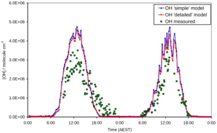
Figures 1 and 2 show the modelled and measured OH con-centrations. The agreement is quite good around midday (10:00–14:00): the models overestimate [OH] by <10% on 7–8 February and <30% on 15–16 February. It should be noted that the concentration of NO is slightly higher on 15 and 16 February (up to 5 ppt) than on 7 and 8 February (up to 3 ppt).

The models reproduce the OH structure, which is due to the passage of clouds, quite well. During these days j(O1D) tracks OH closely; Creasey et al. (2003) reported a high cor-relation (r=0.95) between measured [OH] and the rate of OH production from ozone photolysis during clean days in SOAPEX-2. There is a tendency for the model profiles to overestimate [OH] before and after this midday period (see especially 8 and 16 February). As discussed in Sect. 5.3, the feedback from HO2to OH, via reaction with O3and NO, is

significantly less than formation of OH via ozone photoly-sis, so that a neglected sink is the most likely explanation of this discrepancy, although its identity is not clear. On day 15, there is a significant evening “tail” in the OH concentra-tion, that the model does not reproduce. The “tail” will be discussed further in Sect. 5.2.

Figures 3 and 4 show the scatter plots for the “detailed” model for the four clean days, together with a 1:1 line repre-senting the case of an ideal agreement. The model clearly has a tendency to overestimate the measured [OH]. In particular on 15 and 16 February the scatter plots are well below the 1:1 line, except for low values of OH, which correspond to the evening “tail”. The scatter plots for 15 and 16 February also have the same slope indicating the similarity between the two days. 7 February shows the best agreement between the model and the measurements.

0.0E+00 1.0E+06 2.0E+06 3.0E+06 4.0E+06 5.0E+06 6.0E+06 0:00 6:00 12:00 18:00 0:00 6:00 12:00 18:00 0:00 Time (AEST) [O H ] / m o le cu le cm -3 OH 'simple' model OH 'detailed' model OH measured

Fig. 1. Model-measurement comparison of OH (7–8 February).

0.0E+00 1.0E+06 2.0E+06 3.0E+06 4.0E+06 5.0E+06 6.0E+06 0:00 6:00 12:00 18:00 0:00 6:00 12:00 18:00 0:00 Time (AEST) [O H] / mo le c u le c m -3 OH 'simple' model OH 'detailed' model OH measured

Fig. 2. Model-measurement comparison of OH (15–16 February).

5.2 HO2measured to modelled comparisons

HO2 measurements during SOAPEX-2 were available only

from 9 February onwards due to technical difficulties and so the comparison is possible only for 15 and 16 Febru-ary, under clean conditions. On 15 February measure-ments were from 09:25 until 23:00, on 16 February from 05:40 until 18:15. The late evening and early morn-ing measurements show a concentration of HO2 of about

2×107molecule cm−3_{. The average and maximum}

mea-sured [HO2] are shown in Table 5. The agreement between

the models and the measurements is roughly within a factor of 2 around midday, which is better than was found in pre-vious modelling results for HO2(Carslaw et al., 1999, 2001;

George et al., 1999; Kanaya et al., 2000; Stevens et al., 1997). The agreement between the “simple” and the “detailed” models is also very good (within 5% on all the modelled days). The models calculate a night time HO2concentration

of about 1×107molecule cm−3: however the late evening and early morning measurements are nearly twice this value (Fig. 5), suggesting that the models consistently underesti-mate the night time concentrations. The night time chemistry will be further discussed in Sect. 5.3.

0.0E+00 1.0E+06 2.0E+06 3.0E+06 4.0E+06

0.0E+00 1.0E+06 2.0E+06 3.0E+06 4.0E+06

Modelled [OH] / molecule cm-3

M easur e d [ O H ] / m o le cul e c m -3 Feb 7th OH Feb 8th OH

Fig. 3. Modelled-measured OH scatter plots.

0.0E+00 1.0E+06 2.0E+06 3.0E+06 4.0E+06 5.0E+06

0.0E+00 1.0E+06 2.0E+06 3.0E+06 4.0E+06 5.0E+06

Modelled [OH] / molecule cm-3

M e a s u re d [O H] / m o le c u le c m -3 Feb 15th OH Feb 16th OH

Fig. 4. Modelled-measured OH scatter plots.

The scatter plots of modelled vs. measured [HO2] for the

“detailed” model on 15 and 16 February are shown in Fig. 6. While on 16 February the model/measurements ratio appears to be roughly constant throughout the day, on 15 February the model overestimation appears to be higher at high [HO2] and

gets closer to a 1:1 ratio at low [HO2].

As with OH, there is a tendency to overestimate the con-centrations by a larger factor before and after the midday pe-riod, except for the “tail” on the evening of 15 February. The “HO2tail” is analogous to the one observed in the same

pe-riod (17:30–23:00) for OH and is clearly visible in the scat-ter plot (Fig. 6). As will be shown in Sect. 5.3 the recycling between OH and HO2is rather slow, owing to the low

con-centration of NO. Since the “tail” is present for both radicals, and since the rate of conversion of OH to HO2is much faster

than that from HO2to OH, the most likely origin of the tail is

a neglected source of OH, but no experimental evidence for its origin is available.

The measured [OH]/j(O1D) ratio shows a sudden in-crease of more than an order of magnitude after 18:00 on 15 February, supporting the proposal of an additional OH source. A possibility is the reaction of ozone with biogenic alkenes, but this would require an unrealistic concentration

0.0E+00 5.0E+07 1.0E+08 1.5E+08 2.0E+08 2.5E+08 3.0E+08 3.5E+08 4.0E+08 0:00 6:00 12:00 18:00 0:00 6:00 12:00 18:00 0:00 Time (AEST) [HO 2 ] / m o le c u le c m -3

HO2 'simple' model HO2 'detailed' model HO2 measured

Fig. 5. Model-measurement comparison of HO₂(15–16 February).

0.0E+00 5.0E+07 1.0E+08 1.5E+08 2.0E+08 2.5E+08 3.0E+08 3.5E+08

0.0E+00 5.0E+07 1.0E+08 1.5E+08 2.0E+08 2.5E+08 3.0E+08 3.5E+08

Modelled [HO2] / molecule cm -3 M easu re d [ H O2 ] / m o lecul e c m -3 Feb 15th HO2 up to 1830 hr Feb 15th HO2 1830 - 1927 hr Feb 16th HO2

Fig. 6. Model-measurement HO2scatter plots.

of monoterpenes (of the order of ppm). Though this cannot be completely ruled out, the cause of the “evening tail” of 15 February remains unknown.

5.3 Rates of production and destruction of HOx

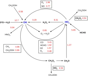
Calculation of the rates of radical production and loss facili-tates an understanding of the key components of the chemical mechanism driving the oxidation chemistry. Figure 7 shows a reaction rate diagram for noon on 7 February. The small imbalances between the rates of production and loss for a given radical reflect the neglect of minor reactions. The rel-ative rates of reactions shown in Fig. 7 are approximately maintained on all four of the days modelled and throughout the daylight hours (06:00–19:00) on those days.

The major source of free-radicals is via O(1D)+H2O,

al-though there is a substantial route to HO2 via HCHO

pho-tolysis. This observation is based on the measured con-centrations of HCHO, which cannot be accounted for by methane chemistry under the conditions pertaining. Ayers et al. (1997) suggested that isoprene might act as a source, but this cannot explain [HCHO] on 7 February, because the measured isoprene concentrations were low (≤2 ppt). The

OH HO₂ CH3O2 CH3O O3 NO H2O2 CO H2 CH4 CH3OOH O2 + H2O O3 HCHO CH3OOH HCHO CH3OOH CH3O2 HNO3 CH3OOH HO2 12.7 1.96 0.77 0.29 0.58 5.41 4.96 1.92 1.57 0.86 0.65 0.48 5.65 1.27 4.54 8.31 0.04 4.54 O1_{D + H} 2O

Fig. 7. Fluxes of free-radicals at 12:00 on 7 February, in units of

105molecule cm−3s−1.

source of HCHO on 7 February is not evident, but it clearly plays an important role in radical initiation.

Termination occurs almost exclusively via peroxy-peroxy reactions (HO2+HO2 and CH3O2+HO2), with very little

formation of HNO3, but with a small contribution from

OH+HO2. The peroxides (H2O2and CH3OOH) act as

mi-nor sources of OH, slightly reducing the effectiveness of the quadratic terminations.

Propagation from OH occurs mainly via CH4 and CO.

The low [NO] drastically reduces the effectiveness of fur-ther propagation from CH3O2 and HO2, with

propaga-tion/termination ratios of 0.22 and 0.17, respectively. For-mation of OH from HO2, which completes the propagation

cycle, occurs principally by reaction with O3, rather than NO,

and the net chain reaction is a sink for ozone. It is difficult to define a simple chain length for the system, because there are two initiation points in the chain cycle. However, defining an approximate chain length as the ratio of the rate of formation of OH via propagation to the total rate of initiation gives a value of only 0.14, emphasising the inefficiency of the chain cycle under these low NOx conditions. The analysis also

confirms the strong correlation between [OH] and j(O1D) (r=0.95), noted by Creasey et al. (2003). While HCHO is a significant radical source, the fraction of HO2so generated

that forms OH is small and OH formation is dominated (78% of the total) by O1D+H2O.

There are close parallels between this analysis and that made for the PEM Tropics A campaign (Chen et al., 2001). The percentage contributions of the main OH forma-tion reacforma-tions were O(1D)+H2O=81% (78%), HO2+O3=5%

(12%), HO2+NO=4% (5%) and CH3OOH+hν=2% (4%) the

SOAPEX-2 results shown in brackets. H2O2photolysis

SOAPEX-2. The dominant OH sinks were CO=34% (34%), CH4=27% (31%) and CH3OOH=11% (5%).

It should also be noted that Chen et al. (2001) used a model with a vertical transport component and they do not specify which height the fluxes they report refer to.

The major difference in the two sets of results relates to the significance of HCHO as a radical source. HCHO was not measured in the P-3B flight in PEM Tropics A and is not quoted as a significant HOxsource, while it contributes 30%

of the total rate of initiation in SOAPEX-2. This discrep-ancy emphasizes the importance of a better understanding the HCHO budget. HCHO was measured during the PEM Tropics B campaign. While it was a HOxsource at higher

al-titudes, for altitudes lower than 1 km it accounted for <5%. Modelled [HO2] is non-zero during the night of 15–16

February (Fig. 5) and shows a slow decay over several hours. HOxand ROxproduction is negligible under these clean

con-ditions, but the chain cycle continues with OH reacting with CO and HO2 with O3. The relative pseudo-first order rate

constants of these reactions, and of OH with CH4, ensure

that [HO2][OH], with [HO2]/[OH] larger than during the

day. Termination occurs via peroxy-peroxy reactions, but is very slow under the night time low radical concentrations, accounting for the long lifetime of the radical pool, which is dominated by HO2. Monks et al. (1996) suggested that night

time [CH3O2] was much greater than [HO2] at Cape Grim

during the SOAPEX-1 campaign, so that CH3O2+CH3O2

and CH3O2+HO2 dominated termination. They assumed

[NOx]=1 ppt. Measurements of [NO] in SOAPEX-2 showed

[NO]<8 ppt during the night of 15–16 February. Under these conditions, the lifetime of CH3O2at night, and as [CH3O2]

falls, becomes determined by CH3O2+NO and propagation

from CH3O2to HO2via CH3O becomes efficient.

5.4 Treatment of aerosol loss in the model

There is substantial uncertainty about the effect of aerosol uptake on OH and HO2concentrations, mainly due to a lack

of ancillary aerosol data recorded during many of the recent MBL campaigns (Carslaw et al., 1999; Kanaya et al., 2000, 2001).

Aerosol surface area is likely to be variable even within a remote marine air mass. Previous MBL aerosol studies describe changes in aerosol concentration and composition due to entrainment from the free troposphere (Bates et al., 1998, 2001; Covert et al., 1998). Raes et al. (1997) found an observable link between vertical transport patterns and aerosol variability in the MBL specifically in the Aitken mode (<0.2 µm). Hence entrainment of aerosol from the free troposphere appears to occur frequently, even in remote MBL air masses. In addition, aerosols have the capacity to travel great distances in the free troposphere, before being entrained into the MBL.

Reactive aerosol surface area (RASA) data were not avail-able for SOAPEX-2 so a constant value of 1.0×10−7cm−1,

representative of clean marine boundary layer conditions was used in the standard model runs described thus far (Whitby and Sverdrup, 1980). In addition, a range of appropri-ate MBL RASA values were calculappropri-ated from literature data (Bates et al., 1998, 2001; Covert et al., 1998; Raes et al., 1997). RASA can be approximated as the total surface area of aerosols, Atot, easily calculated from the mode fit

pa-rameters of lognormal number distributions, RN(the median

droplet radius), Ntot(the total number density of aerosol

par-ticles), and σ (the deviation from the median in a lognormal distribution) (Sander, 1999):

Atot=4π RN2Ntote

2(lg σ )2

(lg e)2 ₍₁₅₎

The mode fit parameters were used to calculate RASAs rep-resentative of the MBL. The parameter, Atot, was calculated

for each aerosol mode and then Atot for each of the modes

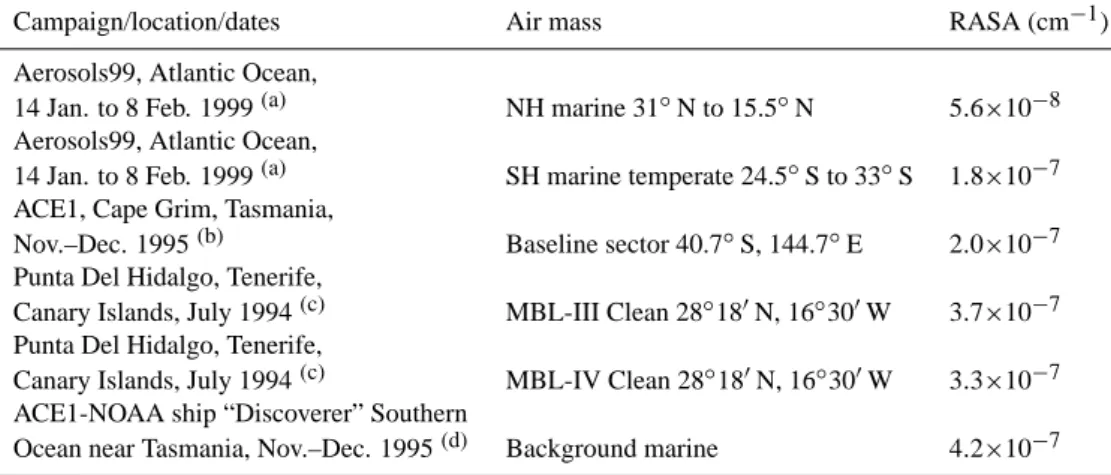
summed to achieve the total RASA for each air mass. A summary of the calculated RASA values with details of the campaign dates and locations are shown in Table 6.

The RASA calculations established a range of values which were included in the detailed model. The lowest relevant value was 5.6×10−8cm−1, measured during the Aerosols99 campaign in the Northern Hemispheric Atlantic Ocean, (Bates et al., 2001). The highest relevant value of RASA was 4.2×10−7cm−1, the background marine value calculated from ship-based measurements near Tasmania (Bates et al., 1998). The larger sea-salt mode dominated as expected in remote MBL conditions. The average RASA value obtained was 2.73×10−7_cm−1_{, significantly higher}

than the value of 1.0×10−7_cm−1 _{quoted by Whitby and}

Sverdrup (1980).

The accommodation coefficients for OH and HO2in our

model are parameterised as temperature dependent accom-modation coefficients (Gratpanche et al., 1996) in Table 3, with no account taken of the surface characteristics. There are a few papers reporting uptake coefficients for both OH and HO2with lower limits quoted for the HO2 coefficients

due to experimental limitations, giving rise to a low confi-dence in current experimental values for HO2 (Cooper and

Abbatt, 1996; Hanson et al., 1992). The impact of reac-tions on aerosol on HO2 concentrations in the remote

at-mosphere could be significant if the uptake coefficient was greater than 0.1, and could dominate if it was close to unity (Saylor, 1997).

When considering the impact of uptake by aerosol, the chemical composition of the aerosol is also likely to be sig-nificant. Bates et al. (1998, 2001) measured strong varia-tions in the chemical composition of the Aitken, accommo-dation and sea-salt dominated coarse modes that would in-fluence the free radical uptake rates, particularly the extent of aerosol acidification. Without data on the size segregated aerosol chemical composition during SOAPEX-2 and the rel-evant laboratory data, it is not possible to calculate accurate accommodation coefficients.

Table 6. Calculated values of RASA.

Campaign/location/dates Air mass RASA (cm−1)

Aerosols99, Atlantic Ocean,

14 Jan. to 8 Feb. 1999(a) NH marine 31◦N to 15.5◦N 5.6×10−8

Aerosols99, Atlantic Ocean,

14 Jan. to 8 Feb. 1999(a) SH marine temperate 24.5◦S to 33◦S 1.8×10−7

ACE1, Cape Grim, Tasmania,

Nov.–Dec. 1995(b) Baseline sector 40.7◦S, 144.7◦E 2.0×10−7

Punta Del Hidalgo, Tenerife,

Canary Islands, July 1994(c) MBL-III Clean 28◦180N, 16◦300W 3.7×10−7

Punta Del Hidalgo, Tenerife,

Canary Islands, July 1994(c) MBL-IV Clean 28◦180N, 16◦300W 3.3×10−7

ACE1-NOAA ship “Discoverer” Southern

Ocean near Tasmania, Nov.–Dec. 1995(d) Background marine 4.2×10−7

(a)_{Bates et al. (2001) mode fit parameters are for the number size distribution at 55% RH from measurements taken during the Aerosols99}

campaign over the Atlantic Ocean.

(b)_{Covert et al. (1998) quote number of aerosol particles as cloud condensation nuclei (CCN) therefore underestimated when assumed equal}

to Ntot. Values for D were estimated from the number-size distribution.

(c)_{Raes et al. (1997).}

(d)_{Bates et al. (1998) values for N}

totand D are quoted at 10% RH.

0.0E+00 1.0E+08 2.0E+08 3.0E+08 4.0E+08 00:00 06:00 12:00 18:00 00:00 06:00 12:00 18:00 00:00 Time (AEST) [H O2 ] / m o le c u le c m -3

Modelled HO2 uptake coefficient = 1, RASA = 4.2e-7, Bates et al. (1998) Modelled HO2 uptake coefficient = 0.1, RASA = 5.6e-8, Bates et al. (2001) Modelled HO2

Measured HO2

Fig. 8. Effect on [HO2] of changing uptake coefficient and RASA

(15–16 February).

The model was run with the RASA at 5.6×10−8cm−1and 4.2×10−7cm−1. The reaction probability for HO2was set

to values of γ =0.1 and 1. The effect on concentrations of HO2 is shown in Fig. 8. It is clear that, except during the

night, the modelled concentrations are much closer to the measurements when the uptake rate was set to a higher value, i.e. with an accommodation coefficient equal to unity and a surface area of 4.2×10−7_cm−1_{. This emphasises the need}

for accurate measurements of the RASA (including chemical composition) during a campaign and better measurements of accommodation coefficients in the laboratory.

Changing the HO2uptake coefficient and the RASA had

little effect on [OH], because the recycling of OH from HO2

-1.0 -0.5 0.0 0.5 1.0 1.5 6:00 9:00 12:00 15:00 18:00 Time (AEST) Sensi ti v it y I ndex H2O j(O1D) j(NO2) O3 NO NO2 CH4 CO HCHO

Fig. 9. Local Sensitivity Analysis of OH between 06:00 and 18:00

(7 February).

is not very efficient in these low NOx conditions as was

shown in detail in Sect. 5.3. Also, the OH uptake coeffi-cient and lifetime are small in comparison to those for HO2

radicals.

5.5 Uncertainty analysis

Sensitivity analysis allows the study of the relationship be-tween the input parameters and the output values of a model (Turanyi, 1990), whereas uncertainty analysis estimates out-put uncertainties from inout-put uncertainties (Saltelli et al., 2000). In order to reduce complexity, the “simple” model was used for the sensitivity and the uncertainty analyses since

-0.6 -0.2 0.2 0.6 6:00 9:00 12:00 15:00 18:00 Time (AEST) Se nsi ti v it y I ndex H2O j(O1D) j(NO2) O3 NO NO2 CH4 CO HCHO

Fig. 10. Local Sensitivity Analysis of HO2 between 06:00 and

18:00 (7 February).

it includes only 92 reactions, yet provides comparable results to the more detailed model.

A brute force local sensitivity analysis was performed by changing the measured concentrations of H2O, O3, NO,

NO2, CH4, CO, HCHO and the values of j(O1D) and j(NO2)

by ±1% and examining the variation in the [OH] and [HO2]

concentrations. The local sensitivity index (SI) was calcu-lated as:

SI =%1X

+1%_−%1X−1%

100 × 0.02 , (16)

where %1X±1% is the percentage variation in the concen-tration of species X when the input parameter is changed by

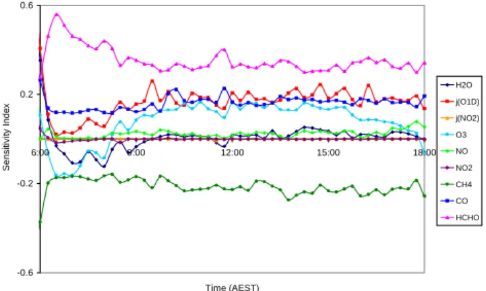
±1%. The results for 7 February are shown in Figs. 9 and 10 for the period 06:00–18:00. The results are in accord with the rate of production analysis. [OH] shows a positive sensitiv-ity to [H2O], j(O1D) and [O3], which directly influence OH

formation and a negative sensitivity to the concentrations of species primarily responsible for its removal, CO and CH4.

[HCHO] shows the largest positive sensitivity for [HO2],

be-cause it acts as a photolysis source. j(O1D), [CO] and [O3]

also have positive sensitivity indices, because of their influ-ence on the rate of formation of OH or on its conversion to HO2. [CH4], on the other hand, shows a negative sensitivity,

because it reacts with OH to form CH3O2, which has a low

probability of forming HO2in low NOxconditions.

The OH sensitivity to HCHO is positive during the early morning-late afternoon and negative in the central part of the day. This is due to the relative importance of HCHO as OH sink and radical source. In the early morning OH+HCHO is comparable to OH+CH3OOH and less than OH+H2 (at

10:00 fluxes are: 1.6, 1.7 and 2.4×105molecule cm−3s−1, respectively), but in the middle of the day OH+HCHO becomes more important than OH+CH3OOH and as

im-portant as OH+H2 (at 14:00 fluxes are: 4.0, 3.4 and

3.8×105molecule cm−3 s−1, respectively). On the other hand j(HCHO) is broader than j(O1D): in the early morn-ing production of HO2by this route becomes the major

rad-0.0E+00 5.0E+04 1.0E+05 1.5E+05 2.0E+05 2.5E+05 3.0E+05

0.0E+00 2.0E+05 4.0E+05 6.0E+05 8.0E+05 1.0E+06

mean std j(O1D) O1D+H2O O1D+N2 [O3] [HCHO] OH+CO OH+CH4 HO2+O3

Fig. 11. Morris One-At-a-Time Analysis of OH for 7 February.

Only the most significant parameters are indicated (std is standard deviation). 0.0E+00 2.5E+06 5.0E+06 7.5E+06 1.0E+07 1.3E+07 1.5E+07 1.8E+07 2.0E+07

0.0E+00 2.0E+07 4.0E+07 6.0E+07 8.0E+07 1.0E+08

mean st d [HCHO] HCHO=CO+2HO2 CH3O2+HO2 HO2+HO2 j(O1D)

Fig. 12. Morris One-At-a-Time Analysis of HO₂ for 7 February Only the most significant parameters are indicated (std is standard deviation).

ical production reaction. In addition since ozone photolysis is slow, HO2+O3 is a significant source of OH. So in the

early morning late afternoon perturbing HCHO affects OH production from HCHO through HO2 more than OH loss,

thus giving a positive SI.

Local sensitivity analysis is of limited value when the chemical system is non-linear. In this case global meth-ods, which vary the parameters over the range of their possi-ble values, are preferapossi-ble. Two global uncertainty methods have been used in this work, a screening method, the so-called Morris One-At-A-Time (MOAT) analysis and a Monte Carlo analysis with Latin Hypercube Sampling (Saltelli et al., 2000; Z´ador et al., submitted, 20041). The analyses were performed by varying rate parameters, branching ratios and constrained concentrations within their uncertainty interval,

1_{Z´ador, J., Pilling, M. J., Wagner, V., and Wirtz, K.:}

Quantita-tive assessment of uncertainties for a model of tropospheric ethene oxidation using the European Photochemical Reactor, Atmos. Env-iron., submitted, 2004.

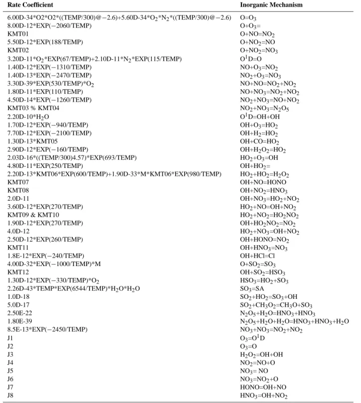
Table 7. Chemical mechanism used in the “simple model”. Notation is in FACSIMILE format (see http://mcm.leeds.ac.uk/MCM/). Rate Coefficient Inorganic Mechanism

6.00D-34*O2*O2*((TEMP/300)@−2.6)+5.60D-34*O2*N2*((TEMP/300)@−2.6) O=O3

8.00D-12*EXP(−2060/TEMP) O+O₃=

KMT01 O+NO=NO2

5.50D-12*EXP(188/TEMP) O+NO2=NO

KMT02 O+NO2=NO3

3.20D-11*O2*EXP(67/TEMP)+2.10D-11*N2*EXP(115/TEMP) O1D=O

1.40D-12*EXP(−1310/TEMP) NO+O3=NO2

1.40D-13*EXP(−2470/TEMP) NO2+O3=NO3

3.30D-39*EXP(530/TEMP)*O2 NO+NO=NO2+NO2

1.80D-11*EXP(110/TEMP) NO+NO3=NO2+NO2

4.50D-14*EXP(−1260/TEMP) NO₂+NO₃=NO+NO₂

KMT03 % KMT04 NO2+NO3=N2O5

2.20D-10*H₂O O1D=OH+OH

1.70D-12*EXP(−940/TEMP) OH+O3=HO2

7.70D-12*EXP(−2100/TEMP) OH+H₂=HO₂

1.30D-13*KMT05 OH+CO=HO2

2.90D-12*EXP(−160/TEMP) OH+H2O2=HO2

2.03D-16*((TEMP/300)4.57)*EXP(693/TEMP) HO2+O3=OH

4.80D-11*EXP(250/TEMP) OH+HO2=

2.20D-13*KMT06*EXP(600/TEMP)+1.90D-33*M*KMT06*EXP(980/TEMP) HO₂+HO₂=H₂O₂

KMT07 OH+NO=HONO

KMT08 OH+NO₂=HNO₃

2.0D-11 OH+NO3=HO2+NO2

3.60D-12*EXP(270/TEMP) HO2+NO=OH+NO2

KMT09 & KMT10 HO2+NO2=HO2NO2

1.90D-12*EXP(270/TEMP) OH+HO2NO2=NO2

4.0D-12 HO2+NO3=OH+NO2

2.50D-12*EXP(260/TEMP) OH+HONO=NO2

KMT11 OH+HNO₃=NO₃

1.8E-12*EXP(−240/TEMP) OH+HCl=Cl

4.00D-32*EXP(−1000/TEMP)*M O+SO₂=SO₃

KMT12 OH+SO2=HSO3

1.30D-12*EXP(−330/TEMP)*O2 HSO3=HO2+SO3

2.26D-43*TEMP*EXP(6544/TEMP)*H2O*H2O SO3=SA

1.0D-18 SO2+HO2=SO3+OH

5.0D-17 SO₂+CH₃O₂=CH₃O+SO₃

2.50E-22 N2O5+H2O=HNO3+HNO3

1.80E-39 N₂O₅+H₂O+H₂O=HNO₃+HNO₃+H₂O

8.5E-13*EXP(−2450/TEMP) NO3+NO3=NO2+NO2

J1 O₃=O1D J2 O3=O J3 H2O2=OH+OH J4 NO2=NO+O J5 NO3= NO J6 NO3=NO2+O J7 HONO=OH+NO J8 HNO₃=OH+NO₂

which were taken from the IUPAC (Atkinson et al., 2001) and JPL evaluations (DeMore et al., 1994) for the kinetic pa-rameters and from the instrumental precision for the mea-sured values.

The MOAT method (Saltelli et al., 2000; Z´ador et al., submitted, 20042) determines the effect of variations of

2_{Z´ador, J., Pilling, M. J., Wagner, V., and Wirtz, K.:}

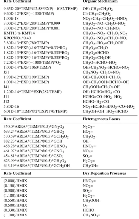
Table 7. Continued.

Rate Coefficient Organic Mechanism

9.65D-20*[email protected]*EXP(−1082/TEMP) OH+CH₄=CH₃O₂

9.60D-12*EXP(−1350/TEMP) Cl+CH4=CH3O2

1.00E-18 NO3+CH4=CH3O2+HNO3

3.00D-12*EXP(280/TEMP)*0.999 CH3O2+NO=CH3O+NO2

3.00D-12*EXP(280/TEMP)*0.001 CH3O2+NO=CH3NO3

KMT13 % KMT14 CH₃O₂+NO₂=CH₃O₂NO₂

KRO2NO3*0.40 CH3O2+NO3=CH3O+NO2

3.80D-13*EXP(780/TEMP) CH₃O₂+HO₂=CH₃OOH

1.82D-13*EXP(416/TEMP)*0.33*RO2 CH3O2=CH3O

1.82D-13*EXP(416/TEMP)*0.335*RO2 CH3O2=HCHO

1.82D-13*EXP(416/TEMP)*0.335*RO2 CH3O2=CH3OH

7.20D-14*EXP(−1080/TEMP)*O2 CH3O=HCHO+HO2

1.00D-14*EXP(1060/TEMP) OH+CH3NO3=HCHO+NO2

J51 CH3NO3=CH3O+NO2

1.90D-12*EXP(190/TEMP) OH+CH₃OOH=CH₃O₂

1.00D-12*EXP(190/TEMP) OH+CH3OOH=HCHO+OH

J41 CH₃OOH=CH₃O+OH

1.20D-14*TEMP*EXP(287/TEMP) OH+HCHO=HO2+CO

J11 HCHO=CO+HO2+HO2

J12 HCHO=H2+CO

5.80D-16 NO3+HCHO=HNO3+CO+HO2

6.01D-18*TEMP@2*EXP(170/TEMP) CH₃OH+OH=HO₂+HCHO

Rate Coefficient Heterogeneous Losses

350.0*AREA*([email protected])*GN2O5 N2O5= 633.24*AREA*([email protected])*GHO2 HO2= 530.59*AREA*([email protected])*GCH₃O₂ CH₃O₂= 882.23*AREA*([email protected])*GOH OH= 458.28*AREA*([email protected])*GHNO₃ HNO₃= 461.97*AREA*([email protected])*GNO3 NO3= 454.81*AREA*([email protected])*GSO2 SO2= 623.99*AREA*([email protected])*GH2O2 H2O2= 643.19*AREA*([email protected])*GCH3OH CH3OH=

Rate Coefficient Dry Deposition Processes

(2.000)/HMIX HNO3= (0.150)/HMIX NO2= (0.500)/HMIX SO2= (1.100)/HMIX H₂O₂= (0.550)/HMIX CH3OOH= (0.500)/HMIX O₃= (0.330)/HMIX HCHO= (1.100)/HMIX CH3NO3=

individual parameters (e.g. rate coefficients, branching ra-tios and measured concentrations) on [OH] and [HO2].

Pa-rameter sets are generated according to the Morris algorithm and the effect of a parameter is calculated from model runs with different values of the given parameter. From numerous model runs the mean and the standard deviation of the effect

oxidation using the European Photochemical Reactor, Atmos. Env-iron., submitted, 2004.

of a parameter is calculated. The mean shows the impor-tance of the parameter, while the standard deviation shows the magnitude of the nonlinearity the parameter change im-plies. The mean effect of each parameter was plotted versus the standard deviation and the plots of 7 February for OH and HO2are shown in Figs. 11 and 12.

The Morris analysis confirms the results of the sensitivity analysis, while the clustering of the points around a single

0 3 6 9 12 15 18 21 24 0 1x106 2x106 3x106 4x106 OH modelled OH measured [O H ] / m o lecu le cm -3 Tim e (AEST)

Fig. 13. Model-measurement comparison of OH with 2σ error bars

(7 February). 0 6 12 18 24 30 36 42 48 0.0 2.0x106 4.0x106 6.0x106 8.0x106 O H m odelled O H m easured [O H ] / m o le c u le c m -3 Tim e (A EST)

Fig. 14. Model-measurement comparison of OH with 2σ error bars

(15–16 February).

curve suggests that non-linear and/or interactive effects are not substantial. For OH, the Morris analysis clearly identifies the importance of OH generation from ozone photolysis and illustrates the importance of reliable j(O1_{D) measurements}

and of the rate coefficients that determine the efficiency of the O1D→OH conversion. The HO2analysis emphasizes the

importance of reliable [HCHO] measurements, of the H atom production channel in HCHO photolysis and of the peroxy-peroxy radical chain termination reactions.

Quantum yields for formaldehyde photolysis have not re-ceived the same attention as those for ozone photolysis and are clearly important even in an unpolluted environment. The absorption spectrum is highly structured and more detailed measurements, under atmospheric conditions, are needed. In this work the uncertainty in HCHO measurements was

es-0 6 12 18 24 30 36 42 48 0 1x108 2x108 3x108 4x108 5x108 HO 2 m odelled HO₂ m easured [H O2 ] / m o lecul e cm -3 Tim e (AES T)

Fig. 15. Model-measurement comparison of HO₂with 2σ error bars (15–16 February).

timated to be ∼50%, which is probably a conservative esti-mate.

The box-models are not expected to correctly calculate the concentration of HCHO, but, given the importance of HCHO as shown by the Morris Analysis, it is interesting to see the effect of not constraining the models to HCHO mea-surements on [HOx]. The “simple” model underestimates

[HCHO] by about a factor of two, but because the main source of HO2is OH and the recycling from HO2to OH is

slow under these conditions (Sect. 5.3), this reduces [HO2]

by 15–25%. The effect is smaller for [OH] concentration (5– 7%).

While the Morris analysis is computationally cheap and fast, it is only a screening method, providing qualitative in-formation. The overall model uncertainty was determined by a Monte Carlo method, coupled with the Latin Hyper-cube Sampling (LHS) technique (Saltelli et al., 2000; Z´ador et al., submitted, 20043). A lognormal distribution was as-sumed for the rate coefficients, a uniform distribution for the branching ratios and a normal distribution for the input pa-rameters (H2O, O3, NO, NO2, CH4, CO, HCHO, j(O1D),

j(NO2), temperature). The means and the variances of the

Monte Carlo simulation outputs were calculated from 500 Monte Carlo runs: assuming a lognormal distribution for the outputs, the 2σ standard deviation of the model was esti-mated to be 30–40% for OH and 25–30% for HO2. The

mea-surement uncertainties were 40% for OH and 50% for HO2

(Creasey et al., 2003). The results are shown in Fig. 13 for 7 February (OH) and in Figs. 14 and 15 for 15–16 February (OH and HO2).

3_{Z´ador, J., Pilling, M. J., Wagner, V., and Wirtz, K.:}

Quantita-tive assessment of uncertainties for a model of tropospheric ethene oxidation using the European Photochemical Reactor, Atmos. Env-iron., submitted, 2004.

Figures 13, 14 and 15 show that the uncertainty ranges for model and measurement overlap for OH except in the evening of 15 February (Fig. 14), where, as noted earlier, the measured OH persists into the evening. The significance of the consistent overestimation by the model does need fur-ther investigation, however, despite the uncertainty overlap. A measure of the statistical significance of the overestima-tion would be of value. The comparison for HO2 (Fig. 15)

is much less satisfactory and there is little uncertainty over-lap at any stage on 16 February, although the agreement on 15 February is better, except in the evening. The Morris analysis suggests that this overestimation may be related to HCHO, but that would require an uncertainty in the mea-sured [HCHO] significantly greater than the estimated value of 50%. A more likely source of the discrepancy is an under-estimation in the model of heterogeneous uptake of HO2, as

discussed above.

Data from a recent campaign (NAMBLEX) in Mace Head, Ireland, suggest that in the MBL halogen oxides, such as IO and BrO, may have a significant impact upon [HO2]. IO

was measured during one of the days investigated, 15 Febru-ary, by DOAS (Table 1) with a maximum concentration of 0.8 ppt. The “simple” model was run with a basic IO mech-anism (IO+HO2, HOI photolysis, HOI heterogeneous loss)

using estimated photolysis rates and simple heterogeneous uptake of HOI (k=A ¯₄cγ with γ =0.6). The effect is that OH increases by ∼10% and HO2decreases by ∼10%. A proper

calculation of the impact of halogen oxides on the [HOx] in

the MBL requires accurate photolysis rates and aerosol up-take rates. This rough calculation shows that the effect of IO is not negligible and is being considered in more detail in the NAMBLEX campaign (where [IO] was generally higher).

6 Summary and conclusions

Two observationally constrained box-models, based on the Master Chemical Mechanism and with different levels of chemical complexity, have been used to study the HOx

rad-ical chemistry during the SOAPEX-2 campaign, which took place during the austral summer of 1999 (January–February) at the Cape Grim Baseline Air Pollution Station in north-western Tasmania, Australia. The box-models were con-strained to the measured values of long lived species and pho-tolysis rates and physical parameters (NO, NO2, O3, HCHO,

j(O1D), j(NO2), H2O and temperature). In addition the

“de-tailed” model was constrained to the measured concentration of CO, CH4and 17 NMHCs, while the “simple” model was

additionally constrained only to CO and CH4. The models

were updated to the latest available kinetic data and com-pleted with a simple description of the heterogeneous uptake and dry deposition processes.

The models were used to calculate [OH] and [HO2] and

the results were compared with the measurements performed by the FAGE instrument. Four days (7, 8, 15, and 16

February) were selected as representative of the extremely clean conditions of the Southern Hemisphere Marine Bound-ary Layer. These very clean conditions (NO<3 ppt) corre-spond to the cleanest conditions under which radical mea-surements have been taken at ground level in the Southern Pacific Ocean. The two models agree to within 5–10% or less.

The agreement between modelled and measured OH is within 10% on 7 and 8 February and 20% on 15 and 16 February around midday. Less satisfactory agreement was obtained for HO2, using a simple heterogeneous

up-take treatment, as the models overestimate it by about 40% on 15 and 16 February. By increasing the uptake coeffi-cients (γ ) for OH and HO2 from 0.1 and 1 and increasing

the reactive aerosol surface area (RASA) to 4.2×10−7 _and

5.6×10−8cm−1, a better agreement with HO2measurements

resulted, with little effect on OH, due to the low NOx

condi-tions of Cape Grim on these days.

A rate of production analysis shows that radical produc-tion occurs primarily via O(1D)+H2O, but with a

signifi-cant contribution to HO2 from HCHO photolysis. OH

re-acts mainly with CO and CH4, followed by HCHO, H2, O3

and CH3OOH with minor contributions from NMHCs. At

the low NO concentrations encountered on these clean days, radical-radical reactions dominate the loss of peroxy-radicals resulting in a reduced chain propagation via CH3O2+NO and

HO2+NO and in a very short chain length (∼0.14),

calcu-lated as the rate of HO2→OH conversion divided by the total

radical production rate.

The rate of production analysis was complemented by a local sensitivity analysis and by a global Morris screening analysis. These analyses demonstrate the necessity of accu-rate measurements of j(O1D) and [HCHO] and reduced un-certainty in the quantum yields for H from HCHO photolysis. Finally, a Monte Carlo method coupled with the Latin Hypercube Sampling (LHS) was used to assess the overall model uncertainty. The 2σ standard deviation of the model was estimated to be 30–40% for OH and 25–30% for HO2,

which is comparable to the instrumental uncertainty.

Acknowledgements. We gratefully acknowledge the support and

the help of the (now) Commonwealth Bureau of Meteorology, of the CSIRO Melbourne and of the Cape Grim staff for during the SOAPEX-2 campaign, particularly L. Porter and J. Britton. We are also grateful to the staff of CSIRO Atmospheric Research. Thanks to G. Evans for technical assistance with the operation of the FAGE instrument during SOAPEX-2 and to the Universities of Leicester

and East Anglia for the use of their data. A.-L. Haggerstone

acknowledges the University of York for a PhD scholarship. R. Sommariva, J. Z´ador and D. J. Creasey acknowledge the University of Leeds for scholarships. D. E. Heard would like to thank The Royal Society for a University Research Fellowship and some equipment funding. Financial support for this project was provided by the NERC, grant GR3/1A447.

References

Allan, B. J., Carslaw, N., Coe, H., Burgess, R. A., and Plane, J. M. C.: Observations of the nitrate radical in the Marine Boundary Layer, J. Atmos. Chem., 33, 129–154, 1999.

Allan, B. J., Plane, J. M. C., and McFiggans, G.: Observations of OIO in the remote marine boundary layer, Geophys. Res. Lett., 28, 1945–1948, 2001.

Atkinson, R., Baulch, D. L., Cox, R. A., Crowley, J. N., Hampson Jr., R. F., Kerr, J. A., Rossi, M. J., and Troe, J.: Summary of Eval-uated Kinetic and Photochemical Data for Atmospheric Chem-istry, IUPAC Subcommittee on Gas Kinetic Data Evaluation for Atmospheric Chemistry, http://www.iupac-kinetic.ch.cam.ac.uk, December 2001.

Ayers, G. P. and Galbally, I.: A preliminary investigation of a boundary layer – free troposphere entrainment velocity at Cape Grim, Baseline 92, Department of Arts, Sport, Environment, Tourism and Territories, Canberra A.C.T., Australia, 1994. Ayers, G. P., Gillett, R. W., Granek, H., de Serves, C., and Cox,

R. A.: Formaldehyde production in clean marine air, Geophys. Res. Lett., 24, 401–404, 1997.

Bates, T. S., Kapustin, V. N., Quinn, P. K., Covert, D. S., Coff-man, D. J., Mari, C., Durkee, P. A., Bruyn, W. J. D., and Saltz-man, E. S.: Processes controlling the distribution of aerosol par-ticles in the lower marine boundary layer during the First Aerosol Characterization Experiment (ACE 1), J. Geophys. Res.-A., 103, 16 369–16 383, 1998.

Bates, T. S., Quinn, P. K., Coffman, D. J., Johnson, J. E., Miller, T. L., Covert, D. S., Wiedensohler, A., Leinert, S., Nowak, A., and Neususs, C.: Regional physical and chemical properties of the marine boundary layer aerosol across the Atlantic during Aerosols99: An overview, J. Geophys. Res.-A., 106, 20 767– 20 782, 2001.

Bauguitte, S.: Rep. ENV4-CT95-0038, Geophys. Inst., University of Bergen, Bergen, Norway, 21–26, 1998.

Bauguitte, S.: Ph.D. Thesis, University of East Anglia, Norwich, UK, 2000.

Behnke, W., George, C., Scheer, V., and Zetzsch, C.: Production

and decay of ClNO2, from the reaction of gaseous N2O5with

NaCl solution: Bulk and aerosol experiments, J. Geophys. Res.-A., 102, 3795–3804, 1997.

Beichert, P. and Pitts, B. J. F.: Knudsen cell studies of the uptake

of gaseous HNO₃and other oxides of nitrogen on solid NaCl:

The role of surface-adsorbed water, J. Phys. Chem., 100, 15 218– 15 228, 1996.

Brasseur, G. P., Hauglustaine, D. A., Walters, S., Rasch, P. J., Muller, J. F., Granier, C., and Tie, X. X.: MOZART, a global chemical transport model for ozone and related chemical tracers 1.: Model description, J. Geophys. Res.-A., 103, 28 265–28 289, 1998.

Brauers, T., Hausmann, M., Bister, A., Kraus, A., and Dorn, H. P.: OH radicals in the boundary layer of the Atlantic Ocean 1.: Mea-surements by long-path laser absorption spectroscopy, J. Geo-phys. Res.-A., 106, 7399–7414, 2001.

Carpenter, L. J., Sturges, W. T., Penkett, S. A., Liss, P. S., Alicke, B., Hebestreit, K., and Platt, U.: Short-lived alkyl iodides and bromides at Mace Head, Ireland: Links to biogenic sources and halogen oxide production, J. Geophys. Res.-A., 104, 1679–1689, 1999.

Carpenter, L. J., Liss, P. S., and Penkett, S. A.: Marine organohalo-gens in the atmosphere over the Atlantic and Southern Oceans, J. Geophys. Res.-A., 108, doi:10.1029/2002JD002769, 2003. Carslaw, N., Creasey, D. J., Heard, D. E., Lewis, A. C., McQuaid,

J. B., Pilling, M. J., Monks, P. S., Bandy, B. J., and Penkett, S. A.:

Modeling OH, HO2, and RO2radicals in the marine boundary

layer – 1. Model construction and comparison with field mea-surements, J. Geophys. Res.-A., 104, 30 241–30 255, 1999. Carslaw, N., Creasey, D. J., Harrison, D., Heard, D. E., Hunter,

M. C., Jacobs, P. J., Jenkin, M. E., Lee, J. D., Lewis, A. C.,

Pilling, M. J., Saunders, S. M., and Seakins, P. W.: OH and HO2

radical chemistry in a forested region of north-western Greece, Atmos. Environ., 35, 4725–4737, 2001.

Carslaw, N., Creasey, D. J., Heard, D. E., Jacobs, P. J., Lee, J. D., Lewis, A. C., McQuaid, J. B., Pilling, M. J., Bauguitte, S., Pen-kett, S. A., Monks, P. S., and Salisbury, G.: Eastern Atlantic Spring Experiment 1997 (EASE97) – 2. Comparisons of model

concentrations of OH, HO2, and RO2 with measurements, J.

Geophys. Res.-A., 107, doi:10.1029/2001JD001568, 2002. Chen, G., Davis, D., Crawford, J., Heikes, B., O’Sullivan, D., Lee,

M., Eisele, F., Mauldin, L., Tanner, D., Collins, J., Barrick, J., Anderson, B., Blake, D., Bradshaw, J., Sandholm, S., Carroll,

M., Albercook, G., and Clarke, A.: An assessment of HOx

chem-istry in the tropical Pacific boundary layer: Comparison of model simulations with observations recorded during PEM tropics A, J. Atmos. Chem., 38, 317–344, 2001.

Cooper, P. L. and Abbatt, J. P. D.: Heterogeneous interactions of

OH and HO₂radicals with surfaces characteristic of atmospheric

particulate matter, J. Phys. Chem., 100, 2249–2254, 1996. Covert, D. S., Gras, J. L., Wiedensohler, A., and Stratmann, F.:

Comparison of directly measured CCN with CCN modeled from the number-size distribution in the marine boundary layer dur-ing ACE 1 at Cape Grim, Tasmania, J. Geophys. Res.-A., 103, 16 597–16 608, 1998.

Creasey, D. J., Heard, D. E., and Lee, J. D.: Eastern Atlantic Spring

Experiment 1997 (EASE97) 1. Measurements of OH and HO2

concentrations at Mace Head, Ireland, J. Geophys. Res.-A., 107, doi:10.1029/2001JD000892, 2002.

Creasey, D. J., Evans, G. E., Heard, D. E., and Lee, J. D.:

Measurements of OH and HO2 concentrations in the

South-ern Ocean marine boundary layer, J. Geophys. Res.-A., 108, doi:10.1029/2002JD003206, 2003.

Cunnold, D. M., Steele, L. P., Fraser, P. J., Simmonds, P. G., Prinn, R. G., Weiss, R. F., Porter, L. W., Langenfelds, R. L., Krummel, P. B., Wang, H. J., Emmons, L., Tie, X. X., and Dlugokencky, E. J.: In situ measurements of atmo-spheric methane at GAGE/AGAGE sites during 1985 to 1999 and resulting source inferences, J. Geophys. Res., 107, D14, doi:10.1029/2001JD001226, 2002.

Davis, D., Crawford, J., Liu, S., McKeen, S., Bandy, A., Thornton, D., Rowland, F., and Blake, D.: Potential impact of iodine on tro-pospheric levels of ozone and other critical oxidants, J. Geophys. Res.-A., 101, 2135–2147, 1996.

DeBruyn, W. J., Shorter, J. A., Davidovits, P., Worsnop, D. R.,

Zahniser, M. S., and Kolb, C. E.: Uptake of Gas-Phase

Sulfur Species Methanesulfonic-Acid, Dimethylsulfoxide, and Dimethyl Sulfone by Aqueous Surfaces, J. Geophys. Res.-A., 99, 16 927–16 932, 1994.