HAL Id: hal-03000126
https://hal.archives-ouvertes.fr/hal-03000126
Submitted on 26 Nov 2020
HAL is a multi-disciplinary open access
archive for the deposit and dissemination of
sci-entific research documents, whether they are
pub-lished or not. The documents may come from
teaching and research institutions in France or
abroad, or from public or private research centers.
L’archive ouverte pluridisciplinaire HAL, est
destinée au dépôt et à la diffusion de documents
scientifiques de niveau recherche, publiés ou non,
émanant des établissements d’enseignement et de
recherche français ou étrangers, des laboratoires
publics ou privés.
PHEBUS on Bepi-Colombo: Post-launch Update and
Instrument Performance
Eric Quémerais, Jean-Yves Chaufray, Dimitra Koutroumpa, François Leblanc,
Aurélie Reberac, Benjamin Lustrement, Christophe Montaron, Jean-François
Mariscal, Nicolas Rouanet, Ichiro Yoshikawa, et al.
To cite this version:
Eric Quémerais, Jean-Yves Chaufray, Dimitra Koutroumpa, François Leblanc, Aurélie Reberac, et
al.. PHEBUS on Bepi-Colombo: Post-launch Update and Instrument Performance. Space Science
Reviews, Springer Verlag, 2020, 216 (4), pp.67. �10.1007/s11214-020-00695-6�. �hal-03000126�
(will be inserted by the editor)
PHEBUS on Bepi-Colombo: Post-launch Update
and Instrument Performance
Eric Qu´emerais · Jean-Yves Chaufray · Dimitra Koutroumpa · Francois
Leblanc · Aur´elie Reberac · Benjamin Lustrement · Christophe Montaron · Jean-Francois Mariscal · Nicolas Rouanet · Ichiro Yoshikawa · Go Murakami · Kazuo Yoshioka · Oleg Korablev · Denis Belyaev · Maria G. Pelizzo · Alan Corso · Paola Zuppella Received: date / Accepted: date
Abstract The Bepi-Colombo mission was launched in October 2018, headed for Mercury. This mission is a collaboration between Europe and Japan. It is dedicated to the study of Mercury and its environment. It will be inserted into Mercury orbit in December 2025 after a 7-year long cruise. Probing of Hermean Exosphere By Ultraviolet Spectroscopy (PHEBUS) is an ultraviolet Spectrograph and is one of the 11 instruments on-board the Mercury Planetary Orbiter (MPO). It is dedicated to the study of the exosphere of Mercury, its composition, dynamics and variability and its interface with the surface of the planet and the solar wind. The PHEBUS instrument contains four distinct detectors covering the spectral range from 55 nm up to 315 nm and two additional narrow windows at 404 nm and 422 nm. It also has a one-degree of freedom mechanism that allows observations along a cone with an half angle of 80◦. This paper follows a detailed presentation of the PHEBUS instrument
design that was presented by Chassefi`ere et al. (2010).
Here we present an update of the science objectives and measurement re-quirements following the results published by the MErcury Surface, Space E. Qu´emerais, J.Y. Chaufray, D. Koutroumpa, F. Leblanc, A. Reberac, B. Lustrement, C. Montaron, J.F. Mariscal, N. Rouanet
LATMOS-OVSQ, 11 boulevard d’Alembert, Universit´e Versailles Saint-Quentin, Guyan-court, France
E-mail: eric.quemerais@latmos.ipsl.fr I. Yoshikawa, G. Murakami, K. Yoshioka Tokyo University, Tokyo, Japan O. Korablev, D. Belyaev IKI, Moscow, Russia
M. Pelizzo, A. Corso, P. Zuppella University of Padova, Padova, Italy
ENvironment, GEochemistry and Ranging (MESSENGER) mission. We also present results of the ground calibration campaigns of the flight unit that is currently on-board MPO.
In the last part, we present some details of the observations that will be performed during the cruise to Mercury, such as stellar observation campaigns, interplanetary background observations and planetary flybys.
keywordsFirst keyword Second keyword More
1 Introduction
The Bepi-Colombo mission is a European Space Agency – Japan Aerospace eXploration Agency (ESA-JAXA) collaboration dedicated to the study of Mer-cury covering all topics from the inner structure to the environment of the planet closest to the Sun. The Bepi-Colombo mission was launched in Oc-tober 2018 and is now on its way to Mercury. This mission is composed of two spacecraft, the Europe-led Mercury Planetary Orbiter (MPO) and the Japan-led Mercury Magnetospheric Orbiter (MMO). PHEBUS, an acronym for Probing the Hermean Exosphere By Ultraviolet Spectroscopy, is an ultra-violet spectrograph on board MPO. It has been developed as a cooperation between three institutes from France, Japan and Russia. Italy provided ground facilities for calibration in the vacuum ultraviolet. The main objective of this instrument is the study of the Hermean exosphere, its composition, dynamics and its interactions with the surface, the magnetosphere and the solar wind.
Like the Moon, and contrary to other terrestrial planets, Mercury is not surrounded by an atmosphere but only by a surface-bounded exosphere, where collisions between atoms are very rare. Because the collisions are very rare, the species are not coupled by collisions as for an usual atmosphere, and each species can be thought as “independent atmospheres” (Stern 1999). The ex-osphere of Mercury was first detected by Mariner 10 during its three flybys. Hydrogen and Helium and their density scale heights were clearly identified from their UV emission lines at 121.6 nm and 58.4 nm, while a measurable signal, with a low signal to noise ratio, attributed to oxygen was also observed at 130.4 nm during the third flyby (Broadfoot et al. 1974, 1976). Later, three other species were detected from Earth by ground-based telescopes : atomic sodium (Potter and Morgan 1985), potassium (Potter and Morgan 1987), and calcium (Bida et al. 2000) from emission lines in the visible range. More re-cently, the UV channel (UVVS, spectral range : 115 – 610 nm) of the Mercury Atmospheric and Surface Composition Spectrometer (MASCS) on MESSEN-GER detected magnesium during its second flyby of Mercury (McClintock et al. 2009) and calcium ions during its third flyby (Vervack et al. 2010). No new species were detected by MESSENGER during most of its orbital period from 18 March 2011 to 30 April 2015. However, during the last Mercury years of the mission, atomic manganese and aluminum were discovered, and the calcium ion (detected only during the third flyby) was finally confirmed (Vervack et al. 2016). At the time when MESSENGER was in orbit around Mercury, iron
and aluminum lines were also detected from Earth by ground-based telescope observations done in 2008 and 2013 (Bida and Killen 2017).
This paper follows the first PHEBUS instrument paper presented by Chas-sefi`ere et al. (2010). The information contained in that paper is still accurate and gives an accurate summary of the design of PHEBUS. We will not repeat the same information here and will only focus on the new results obtained since 2010. Our goal is to give the reader the knowledge necessary to work with PHEBUS data when they become available.
The first part of this paper presents our current view of the exosphere of Mercury, mainly based on the observations of MASCS-UVVS (McClintock et al. 2008). The second section deals with the update of the science objectives and key science issues of PHEBUS. After reviewing the observation require-ments, we will sumarize the instrument design which is still very similar to what was presented in Chassefi`ere et al. (2010). The next section will present the instrument performance results based on ground measurements made with the flight model before launch. The last section will present some of the obser-vations that are planned for PHEBUS during its seven-year cruise to Mercury.
2 Summary of the main results from MESSENGER
Findings from the MESSENGER UVVS instrument are compiled in McClin-tock et al. (2018). In addition to the new species listed above, MESSENGER also regularly observed the previously detected species H, Na, and Ca. How-ever, the emission from O, supposedly detected by Mariner 10 with a lower sensitivity, was not seen during the entire mission of MESSENGER. The de-tection of manganese at the end of the mission through its emission line at 403 nm was unexpected. This emission is close to a potassium line at 404 nm which was not identified (Vervack et al. 2016). Although the potassium lines at 765 and 770 nm have been detected from Earth, the UV line has never been observed. This point is of particular importance because PHEBUS has a near UV channel centered at 404 nm with a of≈ 20nm Full Width at Half Maximum (FWHM), initially dedicated to study this UV potassium line (Chassefi`ere et al. 2010). This channel could be used to study the manganese emission line instead.
2.1 MESSENGER flybys First flyby
During the first flyby on January 14th 2008, MESSENGER/MASCS ob-served the dayside/near terminator emissions of Na and Ca near the planet and the hydrogen dayside emission at high altitude, as well as the extended anti-sunward Na tail formed by the solar radiation pressure. The dayside ob-servation of the hydrogen Lyman α emission during this flyby confirmed the vertical profile measured by Mariner 10 and was consistent with a 420 K exo-spheric temperature similar to Mariner 10. However, the brightness was larger
by a factor of≈3 and possibly sensitive to short time variations (McClintock et al. 2008). The Na tail observations showed a stronger signal in the north than in the south and a relatively weak one in the near equatorial region. The near terminator observations showed a brighter Ca emission in the dawn hemisphere than in the dusk hemisphere (McClintock et al. 2008).
Second flyby
During its second flyby on October 6th 2008, MESSENGER/MASCS ob-served the anti-sunward tail emissions of Na, Ca and Mg. While the Na tail was observed at all scanned altitudes (up to 56,000 km), the Ca and Mg tails were only observed below 19,500 km. The Mg and Na tail showed a double-lobed, north-south enhancement, without a north/south Na asymmetry as observed during the first flyby, while the Ca tail showed an equatorial enhancement. The double-lobed north-south enhancement of Na is in agreement with the ground observations, suggesting a source of sodium from Mercury’s cusps where the surface can be bombarded by energetic ions, and lead to a sputtering induced diffusion enhancement (Mura et al. 2009, Leblanc and Johnson 2010). The dawn/dusk asymmetry of the Ca emission observed during the first flyby was confirmed, while Na emission showed a peak near the north pole and a weaker emission at dawn. The magnesium emission was rather uniform during the dawn/north pole/dusk scan. Models of the magnesium vertical variations in the tail required two populations (a hot : T > 20,000 K and and a cold pop-ulation T < 5000 K), suggesting different sources of magnesium ejection from the surface (Sarantos et al. 2011).
Third flyby
During the last flyby on 29 September 2009, a first identification of a Ca+
line was reported in the anti-sunward tail near the surface only. This Ca+
con-centration in a region tailward of the near-planet reconnection line is due to the transport of Ca+ in the magnetosphere of Mercury. A sodium tail smaller
than during the second flyby was observed which is consistent with the sea-sonal variation of the radiation pressure caused by the eccentric orbit of Mer-cury. Vertical variations indicate a profile with two scale heights for Na and no north/south asymmetry. On the contrary, the scale heights for Ca and Mg were much larger than previously observed, implying significantly larger ener-gies for the source processes and presented a north/south asymmetry possibly associated (for Mg) to the north/south asymmetry of Mg-bearing minerals at the surface. As for the two first flybys, the Ca emission was brightest at the dawn hemisphere near the equator, while the Na emission showed the polar en-hancements as observed during the previous flybys. The magnesium emission presented a weak double-peaked distribution with one peak near the equator and a second one near 50◦N latitude (Vervack et al. 2010).
2.2 MESSENGER in Mercury Orbit
Regular observations of calcium, sodium and magnesium in the exosphere of Mercury were preformed by MESSENGER/MASCS during its four years of
orbiting around Mercury. The main results published from these observations are summarized here.
Note that sodium has only weak emission lines in the UV range that have never been detected. Thus, it is unlikely that PHEBUS will be able to detect the sodium lines. To study calcium emissions, PHEBUS has an additional channel (called NUV Ca) centered at 422 nm. The magnesium line at 285 nm, detected by MASCS, is also in the spectral range of PHEBUS.
sodium observations
The sodium observations showed large seasonal variations of the brightness, but no substantial year to year variation, and no episodic variation, associated to short term changes in the solar wind, as observed several times from Earth (Cassidy et al. 2015). The reported seasonal variations of the sodium brightness (Cassidy et al. 2015), with a maximum near aphelion (True Anomaly Angle = 180◦) were also different from the Mercury disk observations from Earth,
which showed a brightness minimum near aphelion (Potter et al. 2007, Leblanc and Johnson 2010). This difference could be due to geometric differences in the observations from Earth and MESSENGER. The vertical variations above the subsolar point were consistent with one population at a temperature of 1200 K (deduced from the density scale height). Local time variations indicate the presence of a local enhancement of the sodium column density above the “cold-pole” (Cassidy et al. 2016). Such dependency might be due to an accumulation of sodium atoms at these longitudes which are colder in average over one Mercury day due to the 3/2 spin-orbit resonance of Mercury (Soter and Ulrichs 1967).
calcium observations
The brightness enhancement in the dawn hemisphere that was detected during the flybys (and from ground observations) was observed persistently during the orbital phase of MESSENGER and is the dominant morphological feature of the exospheric calcium distribution. This suggests that the source for this species is at dawn. The analysis of the first data suggested that the source was not associated with the magnetosphere nor with a release at dawn from accumulated trapped atoms on the nightside (Burger et al. 2012, 2014). The seasonal variations with a peak near a true anomaly angle (TAA) of 20◦
and a minimum near TAA = 195◦and the absence of large year-to-year
vari-ability of the brightness is consistent with a source from impact vaporization of interplanetary dust associated with an interplanetary dust disk having an inclination less than 5◦ with the respect to the plane of Mercury’s orbit, and a second dust disk associated with the dust trail along the orbit of comet Encke (Killen et al. 2015). The vertical profile of the brightness suggest that the calcium distribution is composed of one population with a temperature of≈ 50,000 K (Burger et al. 2014) in agreement with ground-based observa-tions (Bida et al. 2000). It is possible that it is produced by dissociation of calcium-bearing molecules followed by recombination (Killen and Hahn 2015).
magnesium observations
The accumulated orbital observations from MESSENGER show an en-hancement in magnesium at dawn near perihelion. As for Na and Ca emission,
the dayside Mg emission at low altitude showed large seasonal variations. A peak of column density is observed near TAA = 315◦. One warm population
is usually sufficient to fit the observed profiles, but for a few profiles a sec-ond hotter population is required (Merkel et al. 2017). Variations associated to a magnesium exospheric enhancement above terranes rich in magnesium mapped by the XRS instrument (Weider et al. 2015) have been noticed. Due to the Mercury 3:2 spin-orbit resonance, these terranes are at dawn near per-ihelion only every two years and at dusk the other years, and the magnesium brightness is systematically larger during the years when these terranes are at dawn (Merkel et al. 2018).
3 Science Objectives and Measurement Requirements 3.1 Science Objectives
PHEBUS core scientific objectives aim to better understand the coupling be-tween the surface, the exosphere, and the magnetosphere of Mercury. They can be summarized in the following way:
C1 Composition and vertical structure
Vertical scans of the exospheric brightness will be used to derive compo-sition as well as the scale heights of the different species. Possible variations with altitude would denote the presence of populations generated by different sources, as shown by MESSENGER observations for Mg (e.g., Merkel et al. 2017). Such scans will be performed all over the planet, providing information about composition, temperature and release processes.
C2 Dynamics: exospheric circulation
PHEBUS’s complete local time and latitude coverage will allow the “fol-lowing” of various species from dayside to nightside. For example, on the Moon, the helium distribution follows the law of exospheric equilibrium for non-condensable gases given by “nT5/2is constant” (Benna et al. 2014).
How-ever, on Mercury, the observations by Mariner 10 were not well matched by such a law (Leblanc and Chaufray 2011). New helium observations in the ex-osphere of Mercury should help to better understand the possible differences between the Moon and Mercury. The significant longitude coverage will pro-vide information about local active regions (such as the cusp regions, terranes rich in magnesium, cold pole) as well as transport in the exosphere.
C3 Orbital variation and variations due to transient events By measuring the densities of various species over several Mercury years, it will be possible to separate the effects of different release mechanisms. As an example, the production by interplanetary dust vaporization is seasonally variable while sputtering in cusp regions should be variable on a much shorter timescale, associated with solar wind variations or solar events (Orsini et al. 2018)
Characterizing ions and neutrals in synergy with the Magnetospheric Mer-cury Orbiter (MMO) and other instruments on MPO should allow the study of planetary ions from their formation region in the exosphere (by neutral ionization), through the magnetosphere until escape or re-implantation on the surface.
C5 Escape, source-sink balance, geochemical cycles
Measuring the escape rates of species is of tremendous interest to character-ize, synergistically with the results of geochemical instruments (like the X-ray spectrometer MIXS), the composition of the eroding regolith. Comparing the escape rate and the exospheric density for each species, it will be possible to estimate the residence time of a given species in the regolith-exosphere system, and, more generally geochemical cycles and source/sink balance. At the end, if noble gases are detected, the present outgassing activity may be studied, as well as (tentatively) the history of solar wind particle implantation.
C6 Surface studies
Some observations on the night side of Mercury, especially the permanently shaded regions (PSRs) (Chabot et al. 2012, 2013) will be dedicated to the search for water ice which may be present in some craters at high latitude (Harmon and Slade 1992, Harmon et al. 1994, Neumann et al. 2013, Lawrence et al. 2013). Indeed, some craters close to the poles never receive direct light from the sun and some water ices brought by comets impacting Mercury may have accumulated there. In these permanently shaded regions, the main source of light is the Lyman α radiation caused by the scattering of solar photons by hydrogen atoms in the interplanetary medium (e.g., Qu´emerais et al. 2008). This creates a glow at 121.6 nm (typically between ≈400 – ≈1400 R) which is incident over the entire surface of Mercury. If present, water ice will be detected by variations of the surface albedo at 121.6 nm. Assuming that the mean UV albedo is close to the value of UV plane albedo of the Moon, that is around 4%, we should get a signal around 40R. This signal will vary like the average background emission integrated over the whole sky illuminating the surface at the point of observation. For water ice, the mean albedo at 121.6 nm is close to 2% (Hendrix and Hansen, 2008). Therefore the emission from the surface at Lyman α should lower in presence of water ice. Possible Lyman α albedo variations for some specific surface features, for example the “hollows” regions discovered by MESSENGER and possibly associated to recent volatile activity (Blewett et al. 2011) will be searched at night to provide constraints on the texture or composition of these regions.
C7 Interaction of the interstellar gas with the solar environment. Sky background measurements with PHEBUS at resonance lines of H (102.5 nm, 121.6 nm) and He (58.4 nm) can provide new diagnostics on the interstellar gas in the heliosphere and its interaction with the solar wind, due to the unprecedented vantage points at small solar distance.
3.2 Measurement Requirements
The main measurement objectives of PHEBUS are:
1. To detect new species, including atoms (e.g., O, C, N, S, Si, Ni), noble gas (e.g. Ar, Ne), molecules (e.g., CO, H2O, OH, H2), ions (Mg+, Na+, etc.),
in addition to already detected species (Na, Ca, K, Mg, H, He, Fe, Al, Mn) 2. To measure an average exosphere (number densities and vertical struc-ture), with as many species as possible to be monitored together at different positions of Mercury around the Sun. Averaging over one 8th of Mercury’s year, i.e., on a time scale of≈ 10 Earth days, is appropriate.
3. To measure sudden local and temporal variations of the exosphere con-tent (time scale less than a few hours) at specific times and places of interest. 4. To search for albedo variations of Mercury’s nightside, lit by the inter-planetary H Lyman α glow, at 121.6 nm, in order to search for possible surface ice layers (H2O for example).
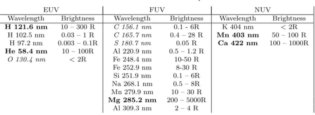
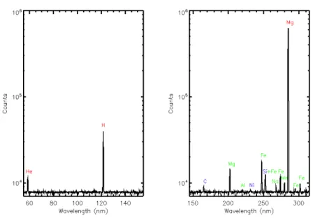
The required maximum uncertainty of the measured abundances is 30%. This includes both systematic and random errors. The required spatial resolu-tion is 15 km. The spectral resoluresolu-tion of the extreme ultraviolet (EUV) range (55-155 nm) is 1 nm and for the far ultra-violet (FUV) (145 – 315 nm) the spectral resolution is 1.5 nm. Two additional near ultra-violet (NUV) detec-tors are implemented to measure the K line at 404 nm and the Ca line at 422 nm. While the 767 nm visible line has been observed regularly from Earth, the emission line at 404 nm has not been detected from MESSENGER-UVVS data, leading to an upper limit of 2R. Instead of the K emission, an unexpected Mn emission has been detected at 403 nm at the end of the mission only, with a brightness of 80 R. This is still in the spectral band of the PHEBUS K NUV detector, so that PHEBUS observations of Mn should be possible. There are other Mn lines in the FUV range (279 nm) that, if detected by PHEBUS, could help us discriminate the K and Mn emission detected with the NUV detector. Different UV emission lines in the spectral range of PHEBUS and their expected brightness are given in Table 1. The simulated accumulated spectra in the EUV and FUV range based on ground calibration are displayed in Fig. 1. Some lines have been detected in the past, while some species have been detected but only at different and brighter lines.
All observed UV emissions show large diurnal and latitudinal variations. As an example, the Ca emission is brighter at dawn, the Na emission inten-sity is stronger near the poles. The one degree-of-freedom pointing device of PHEBUS, with a scanning capability close to the orbit plane, will allow us to achieve a significant latitude and altitude sampling.
4 Instrument Design
The overall design of the PHEBUS instrument is driven by the science objec-tives, the required performance and the allocated resources on the spacecraft. Some trade-offs had to be implemented to find a solution that fulfills all of
Table 1 Estimated brightness range for several main UV emission lines in the exosphere of Mercury. The observed lines are given in bold. The undetected lines of detected species are written in normal text whereas emission lines for undetected species are written in Italics.
EUV FUV NUV
Wavelength Brightness Wavelength Brightness Wavelength Brightness H 121.6 nm 10 – 300 R C 156.1 nm 0.1 - 6R K 404 nm < 2R H 102.5 nm 0.03 – 1 R C 165.7 nm 0.4 – 28 R Mn 403 nm 50 – 100 R H 97.2 nm 0.003 – 0.1R S 180.7 nm 0.05 R Ca 422 nm 100 – 1000R He 58.4 nm 10 – 100R Al 220.9 nm 0.5 – 1.2 R O 130.4 nm < 2R Fe 248.4 nm 10-50 R Fe 252.9 nm 8-30 R Si 251.9 nm 0.1 – 6R Na 268.1 nm 0.5 – 8R Mn 279.9 nm 10 – 30 R Mg 285.2 nm 200 – 5000R Al 309.3 nm 2 – 4 R
these constraints. The general design was presented at the end of the initial study phase by Chassefi`ere at al. (2010). We will not repeat this information here but instead we will focus on the parts that are relevant for the analysis of the PHEBUS data.
4.1 Optical Design
The PHEBUS instrument is a multiple channel instrument composed of two spectrographs operating in overlapping spectral ranges in the ultraviolet (called EUV and FUV) and two near ultraviolet channels dedicated to the calcium (NUV Ca) and potassium (NUV K) line measurements.
For each channel, the spectrographic capability is obtained by use of a slit and a diffraction grating. All Channels share the same collecting area and slit. However, after the slit, the pupil is divided in two halves, one half for the EUV grating (EUV channel goes from 55 nm to 155 nm) and the other half for the FUV grating (FUV channel from 145 nm to 315 nm). The photons measured by the two NUV channels (404 nm and 422 nm) are diffracted by the FUV grating.
A combination of a rotating primary mirror and baffle allows changing the pointing direction of the PHEBUS field of view. The minimal step size and pointing acuracy of the scanner is 0.2◦. The knowledge on the actual position,
as given by the motor encoder, is better than 0.1◦. The line of sight changes with the scanner position along a cone with a half-angle of 80◦and centered on the Y axis of the spacecraft which is the optical axis of the instrument going through the slit. The instrument Field of View is defined by the spectrometer slit size (5.6 x 0.28 mm). With a focal length of 170 mm, it corresponds to ≈ 2◦× 0.1◦ projected on the sky.
Figure 4.1 and Figure 4.1 display the PHEBUS optical and mechanical layouts, respectively. See also Figure 6 in Chassefi`ere et al. (2010).
Fig. 1 Simulated spectra of the exosphere of Mercury observed by PHEBUS using the ground calibration with the EUV channel (left) and FUV channel (right) for an accumulated time of 10000s. The species producing each line is indicated above each detected lines, in red for lines observed in the past, in green for undetected lines of observed species and in blue for undetected species. The density of each species is described with a Chamberlain’s model using surface density and temperature to fit the observations (for observed species). The g factor of each species is computed taking into account the Mercury radial velocity and the Mercury-Sun distance (here 0.31 AU), using the solar flux of Killen et al. 2009 at 1 AU and the NIST database. We consider a line of sight spanning the dayside exosphere with a tangent altitude of 450 km.
The optical plane of the instrument is defined by the position of the slit, gratings and detectors. The optical axis, going through the slit is aligned with the +Y axis of the spacecraft.
Photons from the observed source pass through the baffle and reach the primary mirror. This mirror is made of Silicon Carbide (Sic) with a SiC pow-der coating. It is attached to a scanning mechanism which allows changing of the pointing direction along a cone of 80 degrees half-angle. After reflec-tion by the primary mirror, photons are focused on the slit and reach one of the two holographic gratings that share the pupil. The gratings are made of aluminum with a reflective platinum coating. Their active area size is 4.2 cm by 1.5 cm. Both gratings focus the photons at a position depending on their
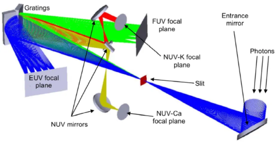
Fig. 2 PHEBUS Optical Layout. Photons from the observed source enter the baffle and reach the primary mirror. After scattering by the primary mirror, the photons are then focused on the slit and reach one of the two holographic gratings that share the pupil. Both gratings focus the photons at a position depending on their wavelength. The two detectors are positioned along the focal planes of the gratings according to the desired spectral range, i.e. 55 nm to 155 nm for the EUV detector and 145 nm to 320 nm for the FUV detector. Note also that both NUV K and Ca photons are caught by two mirrors positioned to the correct spot with respect to the FUV grating. The Y axis of the spacecraft goes from the gratings to the primary mirror through the slit. The plane containing the two detectors and the gratings is the (X,Y) plane of the spacecraft.
wavelength. The two detectors are positioned along the focal planes of the gratings according to the desired spectral range.
Both NUV K and Ca detectors are positioned outside of the optical plane of the instrument. The two Photomultiplier (PM) tubes used in PHEBUS are too big to fit in the space between the two UV detectors. Two small mirrors placed at the correct spot with respect to the FUV grating, direct the photons with the correct wavelength toward a second mirror and the corresponding PM tube.
As seen in Figure 4.1, the PHEBUS field of view is limited by a 21-cm long baffle that allows only light within 8 degrees of the field of view direction to reach the primary mirror. Outside of this guard angle, the attenuation is larger than 7 decades, ensuring that scattered light is minimal. This has been designed to allow for observations of the dayside exosphere of Mercury without getting contamination from the lit surface of the planet.
When the instrument is not operating, the scanner is positioned in front of a parking bracket which blocks the light. This is called the safe position.
Further details on the optical elements were presented in Chassefi`ere et al. (2010).
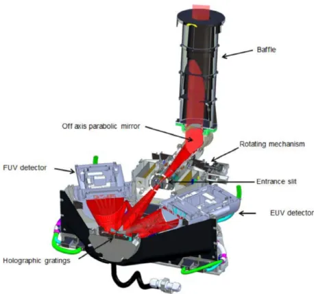
Fig. 3 This is a view of the mechanical layout of PHEBUS where each subsystem has been made visible by cutting the top part away. The light path is shown by the red beam. All elements are at the correct scale. Note that the figure has been rotated by 90 degrees wrt the previous figure to show the dark carbon cover that supports the holographic gratings. That cover was designed to minimize mass. When accommodated on the spacecraft, only the top of the rotating mechanism and the long baffle extend outside of the spacecraft walls.
4.2 Spacecraft Accommodation
As mentioned above, the PHEBUS optical axis going through the slit is aligned with the Y axis of the MPO spacecraft. The rotation axis of the scanner is aligned with the same axis. The PHEBUS rotating baffle sticks out of the radiator side of the spacecraft (-Y side), close to the Nadir side (+Z).
During cruise, at nominal attitude, the spacecraft +Y axis is pointing to-ward the Sun. This means that the radiator side will be on the opposite direc-tion from the Sun. In such a case, the PHEBUS baffle will not be illuminated by the Sun.
Similarly, during the orbital phase of the mission, the radiator side will be aligned with the orbital plane of MPO. This side of the spacecraft will be kept away from the Sun during the complete orbit of Mercury around the Sun. This requires a rotation of the spacecraft by 180 degrees every 44 days and
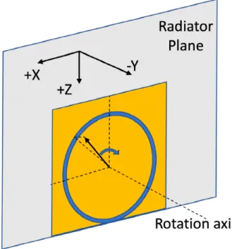
Fig. 4 Sketch of the PHEBUS accommodation on the radiator side of the MPO spacecraft. The yellow area is the area that is covered by the baffle when it is rotating. The zero position of the PHEBUS scanner is centered at 45◦between the +X and -Z axes of the spacecraft. It is shown by the black arrow. The blue circle shows the rotation of the scanner. The blue arrow shows the positive direction, ie. positive angle around +Y.
assures that PHEBUS will be in the shade of the radiator most of the time. The baffle will be in direct illumination from the Sun only during a few days around aphelion and perihelion.
Figure 4.2 shows a sketch of the PHEBUS accommodation on the radiator side of the MPO spacecraft.
4.3 Sub-systems
The PHEBUS sub-systems are described in details in Chassefi`ere et al. (2010). Additional information about the results of the ground measurements will be given below.
5 Instrument Performances 5.1 Sensitivity
The expected count rates measurable by the detectors are between 10−1 and 104counts per second. The lower limit is defined by the dark current variability.
The upper limit is due to the proximity electronics of the detector. Above 104
counts per second the detectors lose linearity.
The EUV channel (55-155 nm) uses a Micro-Channel Plate (MCP) inten-sifier coated with a CsI photocathode. On the ground the photo-cathode was protected by pumping the inside of the detector continuously. After launch, the EUV detector window was opened successfully. The FUV channel uses an MCP intensifier combined with a CsTe photocathode. This channel is vacuum-sealed and much easier to use on the ground as it does not require constant pumping. The cleanliness of the optical elements was maintained on the ground by constant flushing with dry nitrogen.
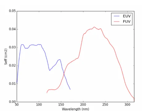
The instrument sensitivity can be expressed as an effective area, which is the product of the entrance area and the spectral efficiency of the instrument. The spectral efficiency is the product of the mirror reflectivity, the grating efficiency and the detector quantum efficiency. Each optical element of PHE-BUS has been characterized on the ground and we have been able to derive a radiometric model that computes the global sensitivity of the instrument by combination of all the individual measurements. In the case of the FUV chan-nel, the instrumental sensitivity has been measured and found consistent with the product of the efficiencies of the three individual elements. For the EUV channel, no measurement of the global efficiency was done on the ground, so we use the product of the three efficiencies measured separately. The effective area for both channels is shown in Figure 5.1 below.
The relation between the measured line brightness I (units of Rayleigh) and the count rate N (units of s−1) is given by
N = I(λ)· Sef f· Ω (1)
One Rayleigh corresponds to 106
4π photons per square centimeter per second
per steradian. The effective area, noted Sef f, is expressed in units of square
centimeter. Figure 5.1 shows the value of the effective area for both EUV and FUV channels. The solid angle of the instrument is noted Ω. Based on results from ground calibrations, the instrument solid angle value is equal to 0.1809 square degrees with the slit and it is equal to 4.088 square degrees without the slit. Some observations will be performed without the slit to increase the signal to noise ratio for weaker emissions, at the expense of spectral resolution. Note that for the EUV channels, there are two sensitivity “regimes”. The short wavelength sensitivity curve is due to the sensitivity of “bare” MCP (below 100 nm), while the long wavelength sensitivity is due to the CsI photo-cathode which peaks around 140 nm. The combination of the two “regimes” creates the dip around 120 nm.
Fig. 5 Instrument sensitivity response showing the expected efficient area of the two chan-nels of PHEBUS. These curves correspond to the Flight Model (updated in 2016). The value for the FUV channel (right hand side) was measured on the ground. The value for the EUV channel was deduced from the individual calibration of each optical element before assembly.
Photon counts are read out from the detector every 2 seconds and trans-mitted to the instrument data processing unit. They can be accumulated in the onboard memory in order to perform long time exposure if necessary, but in this case the risk of data corruption by particle events increases. The inte-gration time is fully programmable, the minimum inteinte-gration duration is 0.01 s and the longest duration is 60 minutes.
5.2 Spectral Resolution
PHEBUS has four distinct channels, covering the spectral range from 55 nm to 315 nm and two additional spectral windows centered around 404 nm and 422 nm. The EUV (55nm-155nm) and FUV (145nm-315nm) overlap between 145 nm and 155 nm.
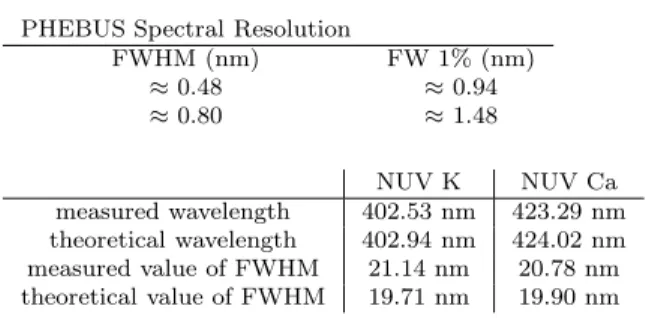
The spectral resolution can be specified for a single isolated line at two levels. The science requirements for PHEBUS specify that the FWHM of an isolated line must be less than 1 nm for the EUV channel, and less than 1.5
PHEBUS Spectral Resolution FWHM (nm) FW 1% (nm) ≈ 0.48 ≈ 0.94 ≈ 0.80 ≈ 1.48 NUV K NUV Ca measured wavelength 402.53 nm 423.29 nm theoretical wavelength 402.94 nm 424.02 nm measured value of FWHM 21.14 nm 20.78 nm theoretical value of FWHM 19.71 nm 19.90 nm
nm for the FUV channel. We have also considered the resolution at the foot of the line, denoted the Full Width at 1% of maximum (FW1%). It must be less than 2 nm for the EUV channel and less than 3 nm for the FUV channel. This ensures that the base of a bright line does not extend too far and contaminate weaker lines of interest in its vicinity. The values obtained from ground measurements for the Flight Model are summarized in Table 5.2. Both EUV and FUV channels fulfill the requirement for spectral resolution.
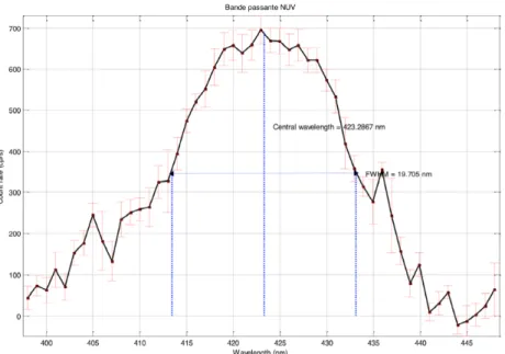
The two Near Ultraviolet channels (NUV) are dedicated to the measure-ment of K and Ca emission lines. One channel is centered around 403 nm and the second one is centered around 424 nm. These two lines are observed with two Photomultiplier Tubes from Hammamatsu. The light beams are re-flected by two mirrors positioned on the side of the FUV grating. The spectral responses of the two NUV channels have been measured on the ground. The re-sults are displayed in Figure 5.2 (K emission line) and Figure 5.2 (Ca emission line) and summarized in Table 5.2.
The ground measurements have shown that the two channels have charac-teristics that are very close to design values. During cruise, the NUV channel sensitivities will be calibrated again for verification. Note that it will not be possible to reevaluate the line center and line width of the spectral response for both channels as no known source is available for that purpose.
5.3 Wavelength Assignment
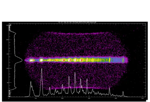
Figure 5.3 shows a typical detector image obtained on the ground with the FUV detector. This ground image is a cumulation of individual measurements. The source is an Argon gas lamp observed in January 2015 at LATMOS facil-ities. The spectrum appears in the middle of the image. The color code shows the intensity for each pixel from purple (low) to white (bright). The image is in binned mode, ie., the resolution (512 x 256) is decreased by a factor of 2 along both dimensions of the original image.
The line on the left of Figure 5.3 shows the result of the horizontal accumu-lation of counts. This corresponds to the intensity along the spatial axis of the slit. The spectrum is spread over horizontal lines 110 to 150 (binned mode). Above and below, only dark counts are observed. Note that the active area of the detector is shown by the presence of dark counts (purple color code). This
Fig. 6 Spectral response of the NUV K Channel, as measured on the ground. The FWHM value is equal to 21.4 nm . This curve has been obtained by illuminating the entrance of the PHEBUS instrument with a monochromatic source at a wavelength varying from 395 nm up to 450 nm and with a spectral width of 0.5 nm .
area is used to determine the dark count level for each image. The line at the bottom shows the spectrum, i.e. the vertical accumulation of the counts over the detector. To increase SNR, it is more useful to accumulate only lines from the area of the detector that is illuminated by the slit.
The Argon lamp contains many spectral lines that are well known. The wavelengths of these lines were tabulated from the NIST spectral data website (https://dx.doi.org/10.18434/T4W30F). Once each line has been identified and its position on the detector has been recorded, we can derive the wave-length assigment on the detector, i.e. the relationship between wavewave-length and the pixel position along the spectral direction. In the first order, this is a linear relationship expressed as
Fig. 7 Spectral response of the NUV Ca Channel, as measured on the ground. The FWHM value is equal to 19.7 nm . This curve has been obtained by illuminating the entrance of the PHEBUS instrument with a monochromatic source at a wavelength varying from 380 nm up to 430 nm and with a spectral width of 0.5 nm .
EUV FUV AXU V (nm) 35.897 356.125
BXU V (nm/pix) 0.263 -0.4835
where P is the pixel number varying from 0 to 511. XU V is either FUV or EUV. The wavelength is expressed in nm.
The same procedure was performed with the EUV detector using a Deu-terium calibration lamp. The results for both detectors are given in Table 5.3.
These values were derived from binned images with a sampling of 512 pixels in the spectral axis. For the full resolution, the total number of pixels in the spectral axis is 1024. This gives us the spectral scale on the detector, which is 0.1315 nm per pixel for the EUV detector and 0.242 nm per pixel for the FUV detector.
Fig. 8 Spectrum of an Argon lamp obtained with the FUV channel of the PHEBUS flight model. Both axes are in detector pixel. This image was obtained in binned mode where the resolution is degraded by binning pixels 2 by 2. This observation was made at LATMOS facilities.
These preliminary results obtained on the ground will be verified during the cruise. There are two reasons for these verifications. First, mechanical and thermal deformations can shift the spectral scale on the detector. Second, these values were determined for one baffle position. However, we expect a small variation of the spectral scale for both detectors when the baffle position is changed. These measurements can be verified by a combination of observations of stars and interplanetary background emission during the cruise. During the primary mission, we expect only minor changes once in orbit around Mercury.
5.4 Field of View and Pointing Direction
The Field of View (FoV) of PHEBUS is defined by the projection of the slit on the sky. When considering that the mirror aberration is negligible, the paraxial FoV is≈ 2◦by 0.1◦. The angular resolution is determined by the width of the
FoV that is ≈ 0.1◦ . Because of the rotation of the primary mirror with the
The FoV direction is represented by 3 vectors in the Unit Reference Frame (URF). The 3 vectors are defined as,
– XF OV defines the direction of the spectral axis (perpendicular to the slit).
– YF OV defines the direction of the spatial axis (along the slit).
– ZF OV defines the direction of the center of the FoV.
The 3 vectors form a right-handed reference frame.
In the URF, the vector coordinates are expressed as follows, where D is the deviation angle of the parabolic entrance mirror (D = 100◦). The position angle of the scanner is equal to S. The zero position of the scanner is defined in front of the parking bracket. As stated earlier, the zero position of the PHEBUS scanner is centered at 45◦ between the +X and -Z axes of the spacecraft.
ZF OV = sinD· cos # S−π4$ cosD − sinD · sin#S−π4$ (3) YF OV = sin 2(D/2) · cos(2S) − sinD · sin#S−π 4 $ − sin2(D/2) · sin(2S) − cos2(D/2) (4) XF OV = YF OV × ZF OV (5)
Here, it is necessary to transform the coordinates in the Unit Reference Frame (URF) into the more useful spacecraft reference frame (MPO). As-suming that there is no misalignment, the transformation is simply expressed as xyMP OMP O zMP O = −zyURFURF xURF (6)
Misalignments of the PHEBUS instrument w.r.t the MPO reference frame will be verified by stellar observations. When the slit is removed, the larger FoV allows to observe stars and to see how their positions on the detector change with the scanner position angle. It is also possible to use a slow drift of the spacecraft attitude which happens during the cruise.
A complete modelling of the instrument optical design shows that a fraction of the photons that reach the detector come from a larger area of the sky than the projection of the slit dimensions. A ray tracing model of the optical design of PHEBUS shows that the nominal area defined by 2◦ along the spatial axis
(YF OV) and 0.1◦along the spectral axis (XF OV) contains 75% of the observed
photons. A rectangular area of 2.3◦ along Y
F OV and 0.4◦ along XF OV and
centered on the FoV direction contains 100% of the photons. The extended area is vignetted with a larger effect as the distance from the nominal slit dimensions increase.
For some observations, it will be possible to remove the slit from the light path to increase the count rate of an extended source or to ensure that a target
is easier to point at. When the slit is removed, the nominal dimensions of the FoV are 2.42◦ along the spatial axis YF OV and 1.2◦ along the spectral axis
XF OV. This nominal region corresponds also to 75% of the photons reaching
the detector for a uniform extended source. To account for all the photons, we have to consider a dimension of 3.3◦ along YF OV and 1.86◦ along XF OV .
The values of the solid angle of the instrument, with and without the slit, were measured on the ground. With the slit, the solid angle is equal to 0.1809 square degree and without the slit it is equal to 4.088 square degree. Because of vignetting on the edge of the Field of View, the measured values are slightly smaller than the expected values of 0.2 square degree with the slit and 6.1 square degree without the slit. These numerical values shoud be taken into account in the modeling of the PHEBUS data.
6 Cruise Observations
During its 7-year cruise to Mercury, the Bepi-Colombo spacecraft will perform 18 full rotations around the Sun, including a flyby of the Earth-Moon system, two flybys of Venus and 6 flybys of Mercury before its final orbit insertion around Mercury in December 2025. Thanks to its accommodation on MPO and its ability to move its scanning mechanism, PHEBUS is able to observe during the cruise outside of the arcs of solar electric propulsion (SEP). And since PHEBUS is placed on the radiator panel of MPO and because this panel is always kept away from the direction of the Sun, PHEBUS is constantly shielded from direct sunlight thus avoiding stray light. Therefore, no special precaution and no special spacecraft attitude are required to operate PHE-BUS safely. There are various targets of interest for a UV spectrograph in the interplanetary space and these targets are presented below.
6.1 Stellar Observations
Stellar observations are the main source of information for the calibration campaign of PHEBUS during the cruise. These observations will allow us to characterize the spectral response of the various channels, if they changed due to the launch campaign and how they may evolve during the cruise to Mercury.
The PHEBUS in-flight calibration can be divided in three phases: – The initial calibration phase after launch
– The cruise phase
– The Mercury orbit phase
The initial calibration phase will allow us to monitor possible changes or contamination that occurred since the ground calibration performed before launch (FUV and NUV detectors). This is essential for understanding the evolution of the instrument sensitivity. The initial calibration will also allow us to measure and verify the alignment of the instrument and the effectiveness
of the baffle rejection (specified at 10−7at 8◦from line center) that is essential
for measurements of the exosphere on the dayside of Mercury.
During the cruise phase, changes will be monitored during the seven years it will take to go to Mercury, and, more importantly, a database of reliable reference spectra will be built and then used during the Mercury orbital phase. Figure 6.1 show examples of the reference spectra built using various sources (data from other instruments and from models) for two stars that should be observable by PHEBUS during the cruise phase as well as during the Mercury orbit phase. These spectra cover both ranges but there are very few sources below 90 nm. Our database of ultraviolet spectra is described in Snow et al. (2013).
During the cruise to Mercury the Y axis of the spacecraft is aligned with the Sun-Spacecraft vector. The +Y axis of MPO is pointing towards the Sun. The spacecraft can rotate around the +Y axis if necessary. Since the radiator panel is on the -Y side, this ensures that the radiator panel is always pointed away from the Sun. Given the PHEBUS accomodation on the radiator panel, this means that the instrument field of view covers a cone centered around the Sun-Spacecraft vector (-Y) with a +80◦ half angle. Thanks to its
scan-ning mechanism, PHEBUS can point to any target along this cone. As the spacecraft orbits around the Sun, the center of the cone also orbits around the Sun accordingly. This means that for a given target that is within 80◦ of
the orbital plane of MPO, there are two possible observations for every Bepi-Colombo orbit around the Sun. This also means that targets within 10◦of the
poles can not be observed. All other targets can be observed 36 times because Bepi-Colombo will orbit the Sun 18 times around the Sun during its full 7-year cruise. The length of time between two possible observations depends on the latitude of the target above the spacecraft orbit plane. Because PHEBUS can-not be operated during the solar electric propulsion arcs which cover roughly half the time, the actual number of observations will come down to 18 in aver-age. In the end, due to spacecraft operation limitations, we expect that each star of interest for the PHEBUS calibration may be observed approximately 10 times, spread over the 7 year cruise to Mercury.
The lower limit for observability of stars will depend on both the maximum integration time and the mean level of dark counts per second. The acceptable limit is defined by the need to have a signal to noise ratio of at least 10 for the accumulated counts per nm during the observation. For typical values of 100 seconds and an expected dark count rate of 0.1 count per second per pixel (conservative estimate), fluxes of at least 100 photons cm−2 s−1 nm−1 are
observable. Lower fluxes are observable for longer integration times.
Based on ground calibration results for the Flight Model unit and the radiometric model, we have determined which stars are good candidates for in-flight calibration. By making observations of known stars during the cruise it will be possible to calibrate PHEBUS detectors with a good relative accuracy (10%). The stellar observations made during the cruise will be used as reference spectra for the in-orbit sensitivity monitoring.
Fig. 9 Calibration stars: Example of spectra in the PHEBUS database. The left panel shows an example that covers the FUV channel and part of the EUV channel. The right panel shows an example for the short wavelengths in the EUV channel.
6.2 Interplanetary observations
A key cruise science objective is to study the distribution of the neutral hy-drogen (HI) and helium (HeI) populations in the interplanetary medium. The origin of the H and He populations in interplanetary space is the so-called Interstellar Wind, a flow of neutral particles (principally hydrogen with about 15% helium and a small portion of oxygen atoms) due to the relative motion of the Sun through the diffuse and partially ionized interstellar gas at ≈ 25 km / s . The supersonic solar wind (SW) carves out a bubble, the heliosphere, through the interstellar plasma, confining the SW plasma inside the helio-sphere while on the outside, the interstellar plasma is diverted around the heliospheric interface. The neutral particles of the interstellar medium have mean free paths of the scale of the heliospheric interface (approximately 100 AU) and can therefore penetrate through this region into the solar system in the form of an interstellar wind in the rest frame of the Sun (see, e.g. Bertaux et al., 1985).
6.2.1 The Neutral H Distribution
The H population is filtered at the heliospheric interface through resonant charge-exchange coupling with protons. This process creates a population of secondary neutral atoms that conserve the local dynamic properties of the shocked interstellar plasma (heating, deceleration, and deflected velocity vec-tor) at the heliospheric interface. A mixture of the two neutral populations (primary and secondary) then propagates into the interplanetary medium with the following initial parameters: direction coordinates in ecliptic≈ (252.5, 8.9) (Upwind direction), bulk velocity V≈22 km s−1 and average gas temperature
T≈12,000 K of the incoming flow (Qu´emerais et al., 1999; Lallement et al., 2005).
Solar H Lyman α photons are effectively backscattered by the interstellar H atoms. Spectral properties of the backscattered Lyman α radiation depend on the velocity and spatial distribution of the interstellar hydrogen inside the heliosphere. Since the distribution of H atoms is disturbed while entering the solar system, then the backscattered Lyman α serves as a source of information about the heliospheric interface structure. One example of the effect of the heliospheric interface is the measured deflection of the interstellar H atoms flow direction as compared with the direction of the interstellar helium flow (see te next subsection for the characteristics of the He component). This is due to the distortion of the global heliospheric interface structure, caused by the interstellar magnetic field. The magnetic field leads to the asymmetry of interstellar plasma flow in the heliospheric interface and this asymmetry is transferred to H atoms through charge-exchange. This fact opens a possibility to estimate the magnitude and direction of the interstellar magnetic field, in addition to the dynamic parameters of the average interstellar H flow.
Interplanetary background scans through high latitudes can also be used to characterize the latitude distribution of solar wind mass flow and to follow its evolution through the solar cycle (Qu´emerais et al., 2006). Indeed, the in-terstellar H neutral atoms are ionized mainly by charge-exchange with solar wind protons, and in a lesser extent by the solar EUV flux. (λ < 91.2 nm). A cavity is carved in the flow, with a shape that reflects the 3D distribution of the solar wind mass flux. Since only the H atoms that have not been ionized may be observed by Lyman α resonance scattering, their distribution (and thus the interplanetary Lyman α background) reflects the solar wind distri-bution and in particular its latitude dependence (the longitude distridistri-bution is averaged out by solar rotation). Monitoring of the 3D solar wind mass flux distribution has been the main goal of the SOHO/SWAN instrument for the last 24 years (Bertaux et al. 1995, Koutroumpa et al. 2019). Measuring the Lyman α interplanetary background will enable the scientific objectives of the SOHO/SWAN instrument of the mission to be extended by PHEBUS obser-vations along the cruise to Mercury will allow to extend the SWAN database. Furthermore, direct comparisons between PHEBUS and SWAN will improve our knowledge of the PHEBUS calibration.
Fig. 10 Helium cone formed by interstellar helium atoms due to gravitational focusing. The position, density and width of the helium cone is a test of the parameters of the interstellar gas and their variability.
6.2.2 The Neutral He Distribution
The helium cross-section for charge-exchange is much smaller than the hy-drogen cross-section and therefore the population that enters the heliosphere preserves the characteristics of the local interstellar medium. The parameters of the He flow have been established as: direction coordinates in ecliptic ≈ (254.5, 5.5) (Upwind direction), bulk velocity V≈26.2 km s−1 and average gas
temperature T≈6,300 K and number density equal to 0.015 cm−3 (Lallement
et al., 2005).
Although both radiation pressure and gravity affect the hydrogen trajec-tories only gravity significantly affects the helium trajectrajec-tories which execute Keplerian orbits and form a focusing cone downstream of the Sun, resulting in a localized downstream enhancement of helium observed annually by Earth orbiting and L1 spacecraft, see Figure 6.2.2 . The exact shape and size of the He cone is dependent on solar activity since He is also ionized by EUV solar photons and, in a lesser extent, by electron impact.
The goal here is to monitor the He cone characteristics with observations of the He resonance line at 58.4 nm during the cruise and in particular with ded-icated scans through the He cone as BepiColombo evolves near the downwind direction (≈75◦ ecliptic longitude). For the currently planned cruise orbit,
the periods most favorable for these observations are November 2019-January 2020, September-October 2020, April-May 2021, and in average every three to four months starting in October 2021 (regions with red points in figure 3). The observation sequences are the same as the one used for the H observa-tions, i.e. full rotation around the –Y axis with +Y pointed toward the Sun. However, the expected signal from the HeI line is smaller than for the HI line and the integration time should be increased accordingly. Therefore when the spacecraft will be close to the He cone we will increase the duration of the observation (1 to 2 hours in total) to get better statistics for the He line.
6.3 Planetary flybys
Planetary flybys offer good oppportunities to check instrument performance and optimize operations during the nominal mission. The first Mercury flyby will happen as early as 2021 and will be followed by 5 flybys that will allow global observations that will not be possible once the spacecraft is locked into Mercury orbit.
The Mercury flybys have not been studied in detail yet, however targets of interest have been identified.
– Scans of Mercury’s exospheric tail: Once in Mercury orbit, PHEBUS will not be able to observe the exospheric tail at all times. We will use the flybys to scan the exospheric tail at different distances from Mercury (up to few tens of Rm, where Rm is the radius of Mercury) in both FUV and EUV
ranges. This should be repeated during the different flybys to reconstruct the tail geometry at different True Anomaly Angles. The spatial resolution should be of the order of Rm up to a few tens of Rm (also to maximize
the S/N) down to a few tens of percent of Rm near the planet. PHEBUS
observations should start at a few tens of Rm from Mercury in order to
integrate the emission on large portions of the tail when looking far from Mercury. These observations will allow characterization of 1) acceleration in the tail induced by solar pressure, 2) escape rates of the observed species, and 3) reconstruction of the time variability of the exosphere induced by solar wind conditions (significant density inhomogeneity in the tail is the signature of change in the exosphere).
– Measurement of the integrated dayside or nightside exosphere emission during a few hours: from a fixed point of view most likely at large dis-tance, measurements of the spatially integrated spectra (no spatial resolu-tion needed) and of their temporal variability. The objective is to track any short time changes, potentially driven by the solar conditions. As the day-side emission is very bright, this should be performed at a large distance from Mercury and with a reduced intensifier gain.
– Imaging of the dayside exosphere with some reduced spatial resolution (of the order of Rm ). We hope to obtain simultaneous imaging of the
high latitude and equatorial regions to study possible global effects in the exosphere. Here again, dayside observations will require careful assessment. Earth and Venus flybys represent a challenge for PHEBUS as these two planets, having dense atmospheres, are expected to be too bright for safe observation in the FUV. As of writing we expect that the Earth observations will be avoided and we should concentrate on observations of the moon in the EUV channel instead.
Although the exosphere of Venus is very bright, observations from a large distance (from a tenth of an AU at least) will be attempted most likely with a reduced gain for the intensifier to avoid damaging the anode detector. The Venus planetary flybys are discussed in Mangano et al. (this issue) and are not repeated here.
References
1. Benna, M., P.R. Mahaffy, J.S. Halekas, R.C. Elphic, and G.T. Delory. (2015) variability of helium, neon, and argon in the lunar exosphere as observed by the LADEE NMS instrument. Geophys. Res. Lett., 42, 3723-3729, doi:10.1002/2015GL064120
2. Bida, T.A., R.M. Killen, T.H. Morgan. (2000) Discovery of calcium in the Mercury’s atmosphere. Nature,404, 159,-161
3. Bida, T.A., and R.M Killen. (2017) Observations of minor species Al and Fe in Mercury’s exosphere. Icarus, 289, 227-238
4. Bertaux, J. L.; Lallement, R.; Kurt, V. G.; Mironova, E. N. (1985) Characteristics of the local interstellar hydrogen determined from PROGNOZ 5 and 6 interplanetary Lyman-alpha line profile measurements with a hydrogen absorption cell Astronomy and Astro-physics, volume 150 n1, pp 1-20
5. Bertaux et al. (1995) SWAN: A Study of Solar Wind Anisotropies on SOHO with Lyman Alpha Sky Mapping Solar Physics, Volume 162, Issue 1-2, pp. 403-439
6. Blewett, D.T. et al.Hollows. (2011) On Mercury: MESSENGER evidence for geologically recent volatile-related activity. Science, 333 (6051) (2011), pp. 1856-1859, 10.1126/sci-ence.1211681
7. Broadfoot, A.L, D.E. Shemansky, and S. Kumar. (1976) Mariner 10: Mercury Atmo-sphere. Geophys. Res. Lett., 3, 577-580
8. Burger, M.H., R.M. Killen, W.E. McClintock, R.J. Vervack, A.W. Merkel, A.L. Sprague, and M. Sarantos. (2012) Modeling MESSENGER observations of calcium in Mercury’s exosphere. J. Geophys. Res., 117, E00L11, doi: 10.1029/2012JE004158
9. Burger, M.H.,R.M. Killen, W.E. McClintock , A.W. Merkel, R.J. Vervack, T.A. Cas-sidy, and M. Sarantos. (2014) Seasonal variations in Mercury’s dayside calcium exosphere. Icarus, 238, 51-58
10. Cassidy, T.A., A.W. Merkel, M.H. Burger, M. Sarantos, R.M. Killen, W.E. McClintock, and R.J. Vervack. (2015) Mercury’s seasonal sodium exosphere: MESSENGER orbital observations. Icarus, 248, 547-559
11. Cassidy, T.A. W.E. McClintock, R.M. Killen, M. Sarantos, A.W. Merkel, R.J. Ver-vack, and M.H. Burger. (2016) A cold-pole enhancement in Mercury’s sodium exosphere. Geophys. Res. Lett., 43, 11, 121-11,128, doi:10.1002/2016GL071071
12. Chabot, N.L., C. M. Ernst, B.W. Denevi, J.K. Harmon, S.L. Murchie, D.T. Blewett, S.C. Solomon, and E.D. Zhong. (2012) Areas of permanent shadow in Mercury’s south polar region ascertained by MESSENGER orbital imaging. Geophys. Res. Lett., 39, L09204, doi: 10.1029/2012GL051526
13. Chabot, N.L., C.M. Ernst, J.K. Harmon, S.L.Murchie, S.C. Solomon, D.T. Blewett, and B.W. Denevi. (2013) Craters hosting radar-bright deposit in Mercury’s north polar region: Areas of persistent shadow determined from MESSENGER images. J. Geophys. Res., 119, 26-36, doi: 10.1029/2012JE004172
14. Chassefi`ere, E., J-L. Maria, J-P. Goutail, E. Qu´emerais, F. Leblanc, et al. (2010) PHE-BUS : A double ultraviolet spectrometer to observe Mercury’s exosphere. Planet. Space Sci., 58, 201-223
15. Gladstone, G.R., K.D. Retherford, A.F. Egan, D.E. Kaufmann, P.F. Miles, J.W. Parker, D. Horvath, P.M. Rojas, M.H. Versteeg et al. (2012) Far-ultraviolet reflectance properties of the Moon’s permanently shaded regions. J. Geophys. Res., 117, E00H04, doi:10.1029/2011JE003913
16. Harmon, J.K., and M.A. Slade. (1992) Radar mapping of Mercury: full-disk images and polar anomalies. Science, 258, 640, doi:10.1026/science.258.5082.640
17. Harmon, J.K., M.A. Slade, R.A. Velez, A. Crespo, M.J. Dryer, J.M. Johnson. (1994) Radar mapping of Mercury’s polar anomalies. Nature, 369, 213-215
18. Hendrix, A.R., and C.J. Hansen. (2008) Ultraviolet observations of Phoebe from Cassini UVIS. Icarus, 193, 323-333
19. Killen, R.M., D. Shemansky, and N. Mouawad. (2009) Expected emission from Mer-cury’s exospheric species, and their ultraviolet-visible signatures. Astrophys. J. Supp. Ser., 181, 351-359
20. Killen, R.M., and J.M. Hahn. (2015) Impact vaporization as a possible source of Mer-cury’s calcium exosphere. Icarus, 250, 230-237
21. Lallement R., Qu´emerais, E.; , Bertaux J.L., Ferron S., Koutroumpa D., Pellinen R. (2005) Deflection of the Interstellar Neutral Hydrogen Flow Across the Heliospheric In-terface Science, Volume 307, Issue 5714, pp. 1447-1449.
22. Lawrence, D.J., W.C. Feldman, J.O. Goldsten, S. Maurice, P.N. Peplowski, B.J. An-derson, et al. (2013) Evidence of water ice near Mercury’s north pole from MESSENGER Neutrons Spectrometer Measurements. Science, 339, 292 doi: 10.1126/science.1229953 23. Leblanc, F., and R.E. Johnson. (2010) Mercury exosphere I. Global circulation model
of its sodium component. Icarus, 209, 280-300
24. Leblanc, F., and J-Y. Chaufray. (2011) Mercury and Moon He exospheres: Analysis and modeling. Icarus, 216, 551-559
25. McClintock, W.E., E.T. Bradley, R.J. Vervack, R.M. Killen, A.L. Sprague, N.R Izenberg, S.C. Solomon. (2008) Mercury’s exosphere : Observations during MESSENGER’s first Mercury flyby. Science, 321, 92
26. McClintock, W.E., R.J. Vervack, E.T. Bradley, R.M. Killen, N. Moawad, A.L. Sprague, M.H. Burger, S.C. Solomon, and N.R. Izenberg. (2009) MESSENGER observations of Mercury’s exosphere : detection of magnesium and distribution of constituents. Science, 324, 610-613
27. McClintock, W.E., T.A. Cassidy, A.W. Merkel, R.M. Killen, M.H. Burger, R.J. Ver-vack, (2018), Observations of Mercury’s Exosphere: Composition and Structure. In S. Solomon, L. Nittler, and B. Anderson (Eds.), Mercury: The View after MESSENGER (Cambridge Planetary Science, pp. 371-406). Cambridge: Cambridge University Press. doi:10.1017/9781316650684.015
28. Merkel, A.W., T.A. Cassidy, R.J. Vervack, W.E. McClintock, M. Sarantos, M.H. Burger, and R.M. Killen. (2017) Seasonal variations of Mercury’s magnesium dayside exosphere from MESSENGER observations. Icarus, 281, 46-45
29. Merkel, A.W., R.J. Vervack, R.M. Killen, T.A. Cassidy, W.E. McClintock, L.R. Nittler, and M.H. Burger. (2018) Evidence of connection Mercury’s magnesium exo-sphere ot its magnesium-rich surface terrane. Geophys. Res. Lett., 45, 6790-6797, doi: 10.1029/2018GL078407
30. Mura, A., P. Wurz, H.I.M. Lichtenegger, H. Schleicher, H. Lammer, D. Delcourt, A. Milillo, S. Orsini, S. Massetti, and M.L. Khodachenko. (2009) The sodium exosphere of Mercury : Comparison between observations during Mercury’s transit and model results. Icarus, 200, 1-11
31. Neumann, G.A., J.F. Cavanaugh, X. Sun, E.M. Mazarico, D.E. Smith, M.T. Zuber, D. Mao, D.A. Paige, S.C. Solomon, C.M. Ernst, O.S. Barnouin. (2013) Brightness and dark polar deposit on Mercury: Evidence for surface volatiles. Science, 339, 296, doi: 10.1126/science.1229764
32. Orsini, S., V. Mangano, A. Milillo, C. Plainaki, A. Mura, J.M. Raines, E. DeAngelis, R. Rispoli, F. Lazzarotto, A. Aronica. (2018) Mercury sodium exospheric emission as a proxy for solar perturbations transit. Scientific Reports, 8, 928
33. Potter, A.E., and T.H. Morgan. (1985) Discovery of sodium in the atmopshere of Mer-cury Science, 229, 651-653
34. Potter, A.E., and T.H. Morgan. (1986) potassium in the atmosphere of Mercury. Icarus, 67, 336-340
35. Potter, A.E., R.M. Killen, and T.H. Morgan. (2007) Solar radiation acceleration effects on Mercury sodium emission. Icarus, 186, 571-580
36. Qu´emerais, Eric, Bertaux J.L., Lallement R., Berth´e M., Kyr ¨ol ¨a E. and Schmidt W. (1999) Interplanetary Lyman α Line Profiles derived from SWAN/SOHO H Cell measure-ments: 1. The Full Sky Velocity Field. Journal of Geophysical Research: Space Physics, Volume 104, 12585-12603
37. Qu´emerais, Eric; Lallement, Rosine; Ferron, St´ephane; Koutroumpa, Dimitra; Bertaux, Jean-Loup; Kyr´’ol´’a, Erkki; Schmidt, Walter (2008) Interplanetary hydrogen absolute ion-ization rates: Retrieving the solar wind mass flux latitude and cycle dependence with SWAN/SOHO maps, Journal of Geophysical Research: Space Physics, Volume 111, Issue A9, CiteID A09114
38. Qu´emerais, E., V. Izmodenov, D. Koutroumpa, and Y. Malama. (2008) Time dependent model of the interplanetary Lyman α glow : applications to the SWAN data. Astronom. Astrophys., 488, 351-359
39. Sarantos, M., R.M. Killen, W.E. McClintock, E.T. Bradley, R.J. Vervack, M. Benna, and J.A. Slavin. (2011) Limits to Mercury’s magnesium exosphere from MESSENGER second flyby observations Planet. Space Sci., 59, 1992-2003
40. Soter,S., and J. Ulrichs. (1967) Rotation and heating of the planet Mercury. Nature, 214(5095), 1315-1316, doi:10.1038/2141315a0
41. Snow Marty, et al., 2013, A new catalog of ultraviolet stellar spectra for calibration. In: Cross- Calibration of Far UV Spectra of Solar System Objects and the Heliosphere, ed. by E. Qu´emerais, M. Snow, R.M. Bonnet. ISSI Scientific Report Series, SR-013 (2013) 42. Stern, A. (1999) The Lunar atmosphere: history, status, current problems, and context.
Rev. Geophys., 37, 4, 453-491
43. Vervack, R.J., W.E. McClintock, R.M. Killen, A.L. Sprague, B.J. Anderson, M.H. Burger, E.T. Bradley, N. Mouawad, S.C. Solomon, and N.R Izenberg. (2010) Mercury’s complex exosphere: results from MESSENGER’s third flyby. Science, 329, 672-675 44. Vervack, R.J., R.M. Killen, W.E. McClintock, A.W. Merkel, M.H. Burger, T.A. Cassidy,
and M. Sarantos. (2016) New discoveries from MESSENGER and insights into Mercury’s exosphere. Geophys. Res. Lett., 43, 11,545-11,551, doi: 10.1002/2016GL071284
45. Weider, S.Z., L.R. Nittler, R.D. Starr, E.J. Crapster-Pregont, P.N. Peplowski, N.W. Denevi, J.W. Head, P.K. Byrne, S.A. Hauk II, D.S. Ebel, and S.C. Solomon. (2015) Ev-idence for geochemical terranes on Mercury: Global mapping of major elements with MESSENGER’s X-Ray spectrometer. Earth and Plan. Sci. Lett., 416, 109-120