Morphogenesis of 3D sheets exploiting a spatial condition

ORIGINAL ARTICLE DOI 10.1007/s10015-006-0395-7

Shuhei Miyashita

Morphogenesis of 3D sheets exploiting a spatial condition

Received and accepted: July 4, 2006

Abstract This article reports on the morphogenesis of

three-dimensional folding sheets in a computer simulation. In order to exploit the topology of these cellular sheets, we introduced a cell connection map, which can prescript cell connections regardless of the changing number of cells. We show that morphogenetic patterns such as exponential growth, self-replication processes, and annihilation pro-cesses can easily be realized just by observing the number of neighbors of each cell. That means that this feat is achieved in a distributed and autonomous way.

Key words Distributed system · Morphogenesis

Introduction

Multicellular organisms consist of large numbers of cells which are able to shape an organism by an intricate web of cell–cell interactions: a process called morphogenesis. As each cell contains the same genome, morphogenesis relies on autonomous and distributed processes with no central-ized control. Although elucidation of the molecular details of morphogenesis has made great progress in biology, an overall picture is still lacking. We hypothesize that morpho-genesis depends on the two following conditions:

1. morphogenesis is an autonomous, distributed process without any centralized control for all cells;

2. in essence, the morphogenesis of living things is basically understood as expanding and folding sheets.

We used these two conditions as guidelines to screen the existing literature of morphogenetic models. Alan Turing’s

reaction–diffusion model1

uses two chemical substances that are able to produce spatial patterns in space. The point of this mechanism is that, in essence, reaction–diffusion mechanisms are the means of breaking the symmetry among homogeneous cells in an autonomous and distrib-uted way.

Focusing on the form of the gastrointestinal tract, Honda2

advocates that in general the form of a multicellular system is realized as two-dimensional sheets rather than three-dimensional solids. Many approaches toward the study of morphogenesis exist, and these can be divided into several types: Lindenmayer grammars,3

cellular automata,4,5 concentration gradients,6

mechanical approaches,7 recur-rent diagram networks to express the bodies of simulated creatures,8

and extended grid space in a graph model.9 How-ever, little attention has been given to the characteristics of form, i.e., the topology of the cellular network.

Model

In our model, we choose the cell as the level of abstraction. The system consists of cells connecting with each other. Cells differentiate depending on the number of neighbors Cells divide and die (cell differentiation) depending on the number of neighbors they have. This is according to the idea that one of the possible biological mechanisms assumed to code the behavior of morphogenesis would be the concen-tration of chemical substances that diffuse into neighboring cells through channels. In other words, their concentrations could reflect the number of neighbors.

Differentiation rules are applied synchronously

These cell behavior rules are applied synchronously in a specific order. After a specific time passes (100 steps), all cells count their neighbors and take action. (The definition

S. Miyashita (*)

Artificial Intelligence Laboratory, Department of Informatics, University of Zurich, Andreasstrasse 15, CH8050 Zurich, Switzerland Tel. +41-44-635-4589; Fax +41-44-635-4507

e-mail: miya@ifi.unizh.ch

This work has presented in part at the 11th International Symposium on Artificial Life and Robotics, Oita, Japan, January 23–25, 2006

of a step is given below.) Once cell division takes place, one cell is divided into four cells. This is in order to sustain the symmetry of the cell network. In cell deletion, a cell is deleted by cutting the connections to its neighbors. Cell–cell mechanical interaction

Cells are expressed as mass points. Links between them are represented as mechanical connections. The mechanical in-teractions are expressed by a spring and damper model. Although it takes time to converge to the form, the form of cell network topology is unique to each sequence. We give the parameters of the system in Table.1. The equation of motion for cell i is expressed in Eq. 1, where subscripts i,j are identification numbers of the cell.

m c k l a g i j j j j ˙˙ ˙ ˙ q +

(

)

(

)

(

)

(

)

(

)

(

)

(

)

(

)

∑

∑

∑

∑

The position of the cell qi is defined as a vector. A cell that

exists in the neighborhood of cell i is denoted as j. Gravity is added to the system in the z-axis direction, and a cross-product force is also added in order to swell the form of the sheet. The differential equation is integrated by the Euler method (∆t = 0.01, 1 step = 30∆t).

A cell connection map is introduced to constrain the form in “a sheet.” Since sustaining adequate topology for cell reconnection after cell division is tricky, we intro-duced a cell connection map, which gives the relations of all cell connections. Figure 1 shows an example of a cell connection map. When a cell is divided, the square corre-sponding to the cell is also divided into four small squares. In Fig. 1, a) and c) correspond to d) and e), respectively. The links are connected if one square touches another square through the edge. As we are interested in how the two-dimensional sheets expand, most external cells, which exist at the edges of the connection map, are fixed in the same positions. Due to this setting, the system grows like an expanding balloon. Although many parameters are decided arbitrarily, the most important thing here is that once a feature of the model is decided, the form converges to a unique form.

Form can be evaluated using a cell connection map The form of living things always relates to their function, and it plays an important role in the evolutionary process, but evaluating form is quite difficult, and sometimes tends to be arbitrary. However, if we evaluate the form by analyz-ing the cell connection map, all cell relations can easily be detected and estimated. We introduced a fitness value (F) (a kind of entropy) which is defined in Eq. 2, where Si denotes

the area of each cell in the cell connection map, with sub-script i being an identification number of the cell.

F N S S i T i = − 1

∑

We set the area of the whole map 1.0. ST to represent the

sum of all areas of the cells. We generalized this value by dividing by the number of cells, N. The characteristics of this fitness value are as follows.

1. The fitness value gets larger when the distribution of the area sizes gets larger.

2. If the sum of areas is same, the larger the number of cells, and the bigger the value becomes.

3. If cell distribution is the same, it does not depend on scale. That means that the value does not depend on the order of morphogenesis.

Simulations and results

By applying several parameter sets, some fundamental mor-phogenetic processes were observed.

Exponential growth

Figure 2 shows examples of the exponential growth of the system: X–Z, side view; X–Y, top view. The cell connection map is described from left to right. (The magnifier is changed in each view.) In the left-hand model (seq. A), we set the rule that if the number of neighboring cells is 0, 2, 4, 6, or 8, then the cell is divided, and if the number is more

Table 1. Sets of parameters

Symbol Definition Value

k Spring coefficient 50

l Spring natural length 50

m Mass 10

c Damper coefficient 30

g Gravity 50

a Cross-product 2000

than 10, the cell is deleted. These rules are applied one after the other, starting with the division rule. The figure shows that simply by counting the neighbors, the system can gen-erate a bent “two-dimensional” morphological form from one single cell. In the right-hand model (seq. B), if the number of neighboring cells is 0, 2, 4, 6, or 8, the cell is divided, and if the number is 1, 3, 5, 7, or 9, the cell is deleted. This time the division rule is applied twice, and then the cell deletion rule is applied once, starting with division rule. Judging from the X–Y and X–Z views, the

form generated by this rule seems to be completely differ-ent from that of seq. A.

Self-replication, annihilation, stop growth

Figure 3 shows the self-replication process. In this model, if the number of neighboring cells is 0, 2, 5, 7, or 9, the cell is divided, and if the number of neighbors is 1, 3, 4, 6, or 8, the cell is deleted. Each group keeps changing the number of

Fig. 2. Exponential growth sequences. Sequence A, all 8 left-hand blocks. Sequence B, top 2 left-hand blocks and all right-hand blocks

cells in its network, and one and four generate new groups. Several models with other parameters showed annihilation and stop-growth behaviors. The simplest model of annihila-tion behavior can be observed when we set the number of neighbors at 0 for cell division and 2 for cell deletion, and apply the division rule and the deletion rule one after the other. The simplest growth saturation model can be ob-served by setting 0 for cell division and any number except 2 for cell deletion.

Discussions

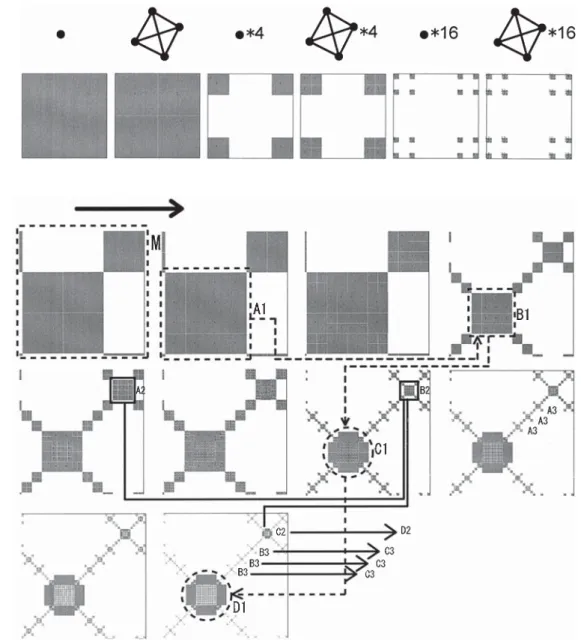
Figure 4 shows a magnification of the part of the cell con-nection map in Fig. 2 marked “M.” After 16 cells appear, which are arrayed in a square grid (A1 and B1), this part of the array becomes rounded (C1). Once this form is created, all internal cells have four neighbors, and thus keep divid-ing. The eight “big” cells surrounding these cells all have at

least 10 cells. Therefore these cells will not divide any more. This is a kind of “expanding bag,” and this bag can be seen in other parts of the body (A2, B2, C2, and A3, B3, C3, and so on). This shows that the system is growing by creating many expanding bags around the body.

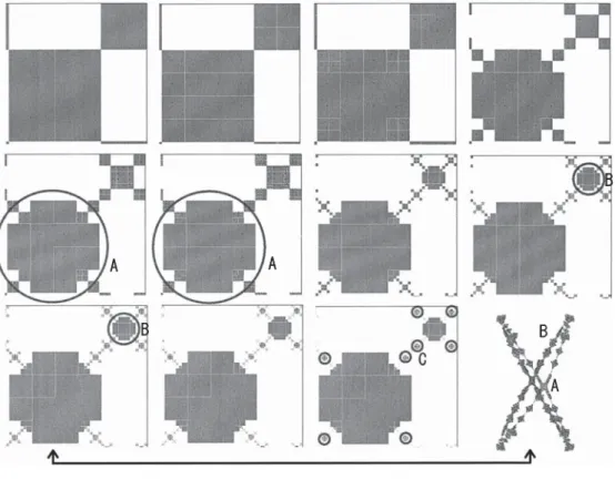
Figure 5 shows the same part of the cell connection map under a different condition of cell division and cell deletion. This time, the cell is divided if the number of neighboring cells is 0, 2, 6, or 8. A cell is deleted if that number is 1, 3, 5, 7, or 9. Although most of the conditions are the same between seq. A and seq. B, the morphogenetic processes are essentially different (see the part marked “A”). Once this shape is created, it does not change any more. That means that the number of cells included in this part does not change. (This is also seen in other parts of sequences B and C, and so on.) This system keeps generating many “gnarls” in different positions. The X–Y view is shown in the same figure. It can be seen that many gnarls are created in the form. The size of each gnarl is the same.

Fig. 3. Self-replication

Fig. 4. Detail of exponential growth sequence B

Fig. 5. Detail of the exponential growth sequence C

We show the graphs for the number of cells and the fitness value in Fig. 6 in order to quantify the difference in the characteristics of these forms between sequences B and C. In Fig. 6 left, the X-axis and the Y-axis represents steps and the number of cells, respectively, when comparing sequences B and C. As the figure shows, the fitness in se-quence B is smaller than that in sese-quence C although the number of cells in sequence B is larger than that in sequence C each time. This means that the uniformity of the whole system of sequence C per cell is larger than that of sequence B. Hence, it suggests that it is not necessary to have many kinds of differentiation rule in order to get complicated forms. In other words, sustaining an adequate cell differen-tiation rule is necessary for the morphogenesis of the model.

Conclusion

These results lead to the following conclusions.

1. Several types of morphogenetic behavior of three-dimensional sheets can be realized in an autonomous and distributed way just by counting the number of neighbors.

2. The form can be quantified easily by evaluating a cell connection map.

Some fundamental morphogenetic behaviors are obser-ved; two types of exponential growth, and self-replication, stop growth, and annihilation processes. These models were

sensitive to the cell differentiation rules, or to put it another way, sensitive to the topology of cell connections. What we intended to show here is the abundant power of morphoge-netic expression supported by the condition of spatial con-straint, and the possibility that we can evaluate complicate forms by mapping them into another method, a cell connec-tion map.

Acknowledgments We thank Peter Eggenberger Hotz for many help-ful suggestions. This research was supported by the Swiss National Science Foundation, project #200021-105634/1.

References

1. Turing AM (1952) A reaction–diffusion model for development. The chemical basis of morphogenesis. Phil Trans R Soc London, Ser B, Biol Sci 237(5):37–72

2. Honda H (2000) The mathematical and physical analysis of morpho-genesis. Kyoritsu-shuppan

3. Lindenmayer A (1968) Mathematical models for cellular interaction in development. J Theor Biol 18:280–300

4. Langton CG (1984) Self-reproduction in cellular automata. Phys D, Nonlinear Phenomena 10(1–2):135–144

5. Gardner M (1970) Mathematical games: the fantastic combinations of John Conway’s new solitaire game, life. Sci Am pp 120–123 6. Wolpert L (1969) Positional information and the spatial pattern of

cellular differentiation. J Theor Biol 25:1–47

7. Odell M, Oster G, Alberch P (1981) The mechanical basis of mor-phogenesis. Dev Biol 85:446–462

8. Sims K (1995) Evolving 3D morphology and behavior by competi-tion. Artif Life 1(4):353–372

9. Tomita K, Kurokawa H, Murata S (2002) Graph automata: natural expression of self-reproduction. Phys D, Nonlinear Phenomena 171(4):197–210