Policy Maker's Credibility with Predetermined Instruments for Forward-Looking Targets

HAL Id: halshs-02371913

https://halshs.archives-ouvertes.fr/halshs-02371913

HAL is a multi-disciplinary open access

archive for the deposit and dissemination of sci-entific research documents, whether they are pub-lished or not. The documents may come from teaching and research institutions in France or abroad, or from public or private research centers.

L’archive ouverte pluridisciplinaire HAL, est destinée au dépôt et à la diffusion de documents scientifiques de niveau recherche, publiés ou non, émanant des établissements d’enseignement et de recherche français ou étrangers, des laboratoires publics ou privés.

Policy Maker’s Credibility with Predetermined

Instruments for Forward-Looking Targets

Jean-Bernard Chatelain, Kirsten Ralf

To cite this version:

Jean-Bernard Chatelain, Kirsten Ralf. Policy Maker’s Credibility with Predetermined Instruments for Forward-Looking Targets. 2019. �halshs-02371913�

WORKING PAPER N° 2019 – 61

Policy Maker’s Credibility with Predetermined

Instruments for Forward-Looking Targets

Jean-Bernard Chatelain

Kirsten Ralf

JEL Codes: B22, B23, B41, C52, E31, O41, O47

Keywords: Determinacy, Proportional Feedback Rules, Dynamic Stochastic General Equilibrium, Ramsey Optimal Policy under Quasi-Commitment

Policy Maker’s Credibility with

Predetermined Instruments for

Forward-Looking Targets

Jean-Bernard Chatelain

Kirsten Ralf

November 14, 2019

Abstract

The aim of the present paper is to provide criteria for a central bank of how to choose among di¤erent monetary-policy rules when caring about a number of policy targets such as the output gap and expected in‡ation. Special attention is given to the question if policy instruments are predetermined or only forward looking. Using the new-Keynesian Phillips curve with a cost-push-shock policy-transmission mechanism, the forward-looking case implies an extreme lack of robustness and of credibility of stabilization policy. The backward-looking case is such that the simple-rule parameters can be the solution of Ramsey optimal policy under limited commitment. As a consequence, we suggest to model explicitly the rational behav-ior of the policy maker with Ramsey optimal policy, rather than to use simple rules with an ambiguous assumption leading to policy advice that is neither robust nor credible.

JEL classi…cation numbers: B22, B23, B41, C52, E31, O41, O47.

Keywords: Determinacy, Proportional Feedback Rules, Dynamic Stochastic General Equilibrium, Ramsey Optimal Policy under Quasi-Commitment.

1

Introduction

Throughout the years, a large number of policy rules for the central bank have been proposed. The aim of the present paper is to provide criteria of how to choose among these di¤erent rules and how to decide in the mathematical modeling whether the policy instrument should be de…ned as forward looking or predetermined and its relation to the policy target. In this context, we will compare simple rules with a predetermined policy instrument, simple rules with a forward-looking instrument, and Ramsey optimal policy with quasi commitment in a model with the new-Keynesian Phillips curve as the transmission mechanism (Gali (2015). Special importance is given to the problem of robustness and the existence of bifurcations.

In a …rst part it will be argued that one cannot deduce from a proportional simple feedback rule, i.e. a rule in which the instrument is a linear function of the deviations of Paris School of Economics, Université Paris I Pantheon Sorbonne, PSE, 48 boulevard Jourdan, 75014 Paris. Email: jean-bernard.chatelain@univ-paris1.fr

y_{ESCE International Business School, Inseec U. research center, 10 rue Sextius Michel, 75015 Paris,}

the policy targets from their long-run equilibrium, that the policy instrument is necessarily a forward-looking variable if the policy target is a forward-looking variable. An example of a simple rule is given in Leeper (1991) where the Central Bank’s short-term interest rate responds linearly to in‡ation deviations. A variable is forward-looking in an equation not derived from intertemporal optimization, such as a proportional feedback rule, if two conditions are satis…ed: Firstly, the variable should depend on its own expectations, and not only on the expectations of other variables. Secondly, these expectations should not be driven by adaptive expectations. Because these simple proportional rules do not include the expectations of the policy instrument itself, one cannot claim it is obvious that the policy instrument is a forward-looking variable.

This assumption matters a lot for policy recommendation. Simple rule theorists solve their model imposing Blanchard and Kahn’s (1980) determinacy condition following an algorithm in three steps (Leeper (1991)):

Firstly, they count the number of predetermined variables.

Secondly, the found number implies the number of stable eigenvalues inside the unit circle for discrete-time models.

Thirdly, the choice of stable and unstable eigenvalues implies a range of values of policy-rule parameters for a given policy-transmission mechanism which is labeled de-terminacy area. This dede-terminacy area corresponds to policy advice for policy-rule pa-rameters. This third implication is an outcome of Wonham’s (1967) theorem. For a controllable system, the parameters of the characteristic polynomial determining these eigenvalues are a¢ ne functions of policy-rule parameters. Eigenvalues within the unit circle correspond to a bounded interval of values speci…c to each policy-rule parame-ter. Conversely, the values of each policy rule-parameter outside their speci…c bounded interval corresponds to eigenvalues outside the unit circle.

What is missing, however, in some of the seminal papers using simple rules (Leeper (1991), Clarida, Gali and Gertler (1999), Woodford (2003), Gali (2015)), is the discussion of why the policy instrument is a forward-looking variable instead of a "backward-looking" or "predetermined" variable when its responds to the deviations of forward-looking policy targets from their set point. From their computation of the number of stable eigenval-ues, the reader can only infer that they implicitly assumed that policy instruments are always forward-looking for simple rules. If policy instruments are counted as predeter-mined variables, the number of eigenvalues inside the unit circle increases. The range of values of policy rule-parameters leading to determinacy is di¤erent. Finally, policy recommendations are di¤erent.

The second contribution of this paper is to highlight the consequences of assum-ing policy instruments forward-lookassum-ing instead of predetermined for a simple rule with forward-looking policy targets. We consider the new-Keynesian Phillips curve as a mone-tary policy transmission mechanism (Gali (2015)). There is an extreme lack of robustness and of credibility if one assumes that policy instrument is forward-looking when at least one policy target is forward-looking in a proportional feedback simple rule.

Cochrane (2019, p.345) expressed his concern of the lack of robustness and of credi-bility:

To produce those equilibria, the central bank commits that if in‡ation gets going, the bank will decrease interest rates, and by doing so it will increase subsequent in‡ation, without bound. Likewise, should in‡ation be less than the central bank wishes, it will drive the economy down to the liquidity trap...

No central bank on this planet describes its in‡ation-control e¤orts this way. They uniformly explain the opposite. Should in‡ation get going, the bank will increase interest rates in order to reduce subsequent in‡ation. It will induce stability into an unstable economy, not the other way around. I have not seen selecting among multiple equilibria on any central bank’s descriptions of what it does... That the central bank will react to in‡ation by pushing the economy to hyperin‡ation seems an even more tenuous statement about people’s beliefs, today and in any sample period we might study, than it is about actual central bank behavior.

The assumption of forward-looking policy instruments for forward-looking policy tar-gets in a simple rule corresponds to the complete lack of credibility of the policy maker. This makes sense: If a policy maker does not care at all about the future in his loss func-tion and in the policy transmission mechanism, he does not care to leave the economy with locally unstable dynamics of policy targets on future dates. Local unstability will markedly increases his loss function in the near future if he does not know the parameters of the policy transmission mechanism with an in…nite precision. Conversely, policy rules which destabilize the future dynamics of policy targets are not credible for the private sector.

With some credibility, the initial value of the current policy instrument (the funds rate) anchors the initial value of the forward-looking policy target (in‡ation) using the feedback rule. Hence, there is no longer the indeterminacy of initial in‡ation. Therefore, it does not make sense to destabilize in‡ation dynamics to rule out indeterminacy. It follows that the assumption of forward-looking policy instruments for forward-looking policy targets provides useless policy recommendations for policy makers who are usually willing to care about the future.

Including ad-hoc equations such as a simple proportional feedback rule for some agents without leads or lags of the policy instruments, leads to ambiguous and misleading results in rational expectations models. Therefore, introducing an asymmetry between a ratio-nal private sector doing intertemporal optimization and an ad-hoc policy rule for policy makers is not a good idea. Modeling the rational behavior of the policy maker would have avoided these lacks of robustness and credibility.

Accordingly, assuming the policy instrument to be backward-looking may correspond to a reduced form of the optimal model of limited commitment, when the policy maker has a non-zero probability to take into account private sector’s expectations (Roberds (1989), Schaumburg and Tambalotti (2007))). This maintains an order of stable dynamics (a number of stable eigenvalues inside the unit circle) which corresponds the order of the dynamics of the private sector’s policy targets. This guarantees the local stability of the dynamics in the space of the policy targets.

To sum up, the lack of robustness and of credibility of simple rules is an artefact grounded by a never discussed conventional assumption: policy instruments are assumed to be forward-looking when they respond to forward-looking policy targets in proportional feedback simple rules.

The rest of the paper proceeds as follows: Section two recalls the mathematical proper-ties of dynamical models putting a special importance on the concepts of predetermined versus non-predetermined variables, determinacy versus indeterminacy, feedback rules, and the convention of de…ning the policy instrument as a forward-looking variable. Sec-tion three compares the policy maker’s soluSec-tions assuming either the policy instrument to be predetermined or to be backward-looking for a new-Keynesian Phillips curve and a cost-push shock transmission mechanism. Section four concludes.

2

Mathematical modeling and economic

interpreta-tion

2.1

Predetermined versus non-predetermined variables

One of the …rst questions when choosing the variables in an economic model is the question of whether these variable are predetermined or not. Some variables, such as the stock of capital, seem to be natural candidates for predetermined variables, for others the decision is more di¢ cult. From a mathematical point of view, any variable can be predetermined or non-predetermined. Blanchard and Kahn’s (1980) start their analysis of a dynamical

system stating that the matrices A and of their dynamic model are ad hoc given

matrices, i.e. not derived from intertemporal optimal choice. The transition matrix A has a given number n of stable eigenvalues inside the unit circle and a remaining number

m of unstable eigenvalues outside the unit circle. They de…ne predetermined

(backward-looking) variables and non-predetermined (forward-(backward-looking) variables and their model as follows:

“The model is given as follows: Xt+1

tPt+1

= A Xt

Pt

+ Z_t; Xt=0 = X0 (1)

where X is an (n 1)vector of variables predetermined at t; P is an (m 1)

vector of variables non-predetermined at t; Z is an (k 1)vector of exogenous variables;tPt+1is the agents expectations of Pt+1held at t; A, are (n + m)

(n + m) and a (n + m) k matrices, respectively.

tPt+1 = Et(Pt+1 p t) : (2)

where Et( ) is the mathematical expectation operator; t is the information

set at date t,.... A predetermined variable is a function only of variables

known at date t, that is of variables in t that Xt+1 = tXt+1 whatever the

realization of the variables in t+1. A non-predetermined variable can be

a function of any variable in t+1, so that we can conclude that Pt+1=tPt+1

only if the realization of all variables in t+1 are equal to their expectations

conditional on t.” Blanchard and Kahn (1980), p.1305.

Blanchard and Kahn (1980) thus assume that the property of whether a variable is predetermined or forward-looking and their respective numbers n and m is given. In practice, they allow that n, m, n, m are discretionary ad hoc choices done by the researcher as it is done by other ad hoc linear rational expectations models of the 1970s. As an example they give an ad hoc multiplier accelerator model including only one non-predetermined (or forward-looking or jump) variable: output (example 4). They show that a researcher can choose which variable is a predetermined or a non-predetermined variable and that this choice is independent from an economic criterion such as real versus nominal variables (p.1307):

This example also shows the absence of necessary connection between "real," "nominal" and "predetermined," "non-predetermined".

Set aside this sentence, Blanchard and Kahn’s (1980) paper does not provide any cri-terion for deciding when a variable is forward-looking or not. In their example of the mul-tiplier accelerator model, the demand components of output: consumption, investment and government expenditures may all have been assumed to depend on forward-looking speci…c expectations of consumption, investment and government expenditures, instead of depending only on aggregate output expectations.

2.2

Optimal control and feedback rule

The next choice of the researcher when modeling monetary policy concerns the type of feedback rule of the central bank. Currie and Levine (1985), Leeper (1991), Clarida, Gali and Gertler (1999), Woodford (2003) and Gali (2015) add to Blanchard and Kahn’s (1980) dynamic system at least one policy instrument it with non-zero correlation (B 6= 0) with

policy targets (Xt; Pt): Xt+1 tPt+1 = A Xt Pt + Z_t+ Bit; Xt=0= X0: (3)

In their examples, Kalman controllability, i.e. the property that policy instruments have a direct of indirect e¤ect on the policy target, is satis…ed:

rank B; AB; A2B; :::An+m 1B = n + m:

The policy maker’s rule is assume to be an ad hoc (behavioral) proportional feedback rule or "simple rule" with policy-rule parameters FX, FP and FX:

it= FXXt+ FPPt+ FZZt: (4)

Restrictions on the policy-rule parameters are often imposed. For example, Leeper’s (1991) interest-rate rule responds only to forward-looking in‡ation and to an exogenous auto-regressive variable (FX = 0).

These proportional feedback rules exhibit no dynamics:

- The policy instrument it does not depend on its lagged values it 1; it 2::. It is not

included in the set of predetermined variables in the …rst row of Blanchard and Kahn (1980) system: Xt+1= AnnXt+ :::where Ann is the upper left n n square block matrix

in matrix of matrix A.

- The policy instrument it does not depends on its expected value: tit+1= Et(it+1). It

is not included in the set of non-predetermined (forward-looking) variables in the second

row of Blanchard and Kahn (1980) system: tPt+1 = AmmPt + ::: where Amm is the

bottom right m m square (block matrix of matrix A.

The following choice of a policy rule, however, would allow the policy instrument to be forward looking or backward looking:

it= FXXt+ FPPt+ FZZt+ 1it 1+ 2it 2+ ::: + b1Et(it+1) : (5)

If the policy instrument depends on its lagged value i 6= 0 and not on its expectation

b1 = 0, then it is a backward-looking variable. If the variable does not depend on its

lagged value i = 0, but it depends on its expected value b1 6= 0 and the expectations

are not adaptive expectations, i.e. its expected value does not depend on the current and lagged values of the policy instrument so that they "cause" the current value it, then itis

on its lagged value i 6= 0 and also on its expected value b1 6= 0, the policy instrument it

is still assumed to be forward-looking variable (Chatelain and Ralf (2018)).

If the feedback rule has no dynamics such that i = 0 and b1 = 0, the above cited

de…nitions of predetermined versus non-predetermined variables of Blanchard and Kahn (1980) do not imply that the policy instrument is forward-looking when at least one policy target is forward-looking.

2.3

Determinacy versus indeterminacy

An important feature of a rational expectations equilibrium in a dynamic model is the indeterminacy or determinacy of the perfect foresight dynamics. Determinacy requires the steady state equilibrium to be locally unique, whereas in the case of indeterminacy a large number of nonstationary solutions of the dynamical system converging to the steady state exist. Then it is for the individual of no importance which future state of nature he expects because for any choice of today’s actions the economy approaches the steady state, no rational decision is possible. To avoid this kind of ambiguity, Blanchard and Kahn (1980) set a stability boundary condition in the in…nite horizon, like the in…nite horizon transversality conditions assumed in optimal control and derive conditions for determinacy, indeterminacy and for a bounded solution:

“This condition in e¤ect rules out exponential growth of the expectations of Xt+1 and Pt+1 held at time t. (This in particular rules out "bubbles"...).”

Blanchard and Kahn (1980), p.1307.

“Proposition 1: If m = m, i.e., if the number of eigenvalues of A outside the unit circle is equal to the number of non-predetermined variables, then there exists a unique solution.” Blanchard and Kahn (1980), p.1308.

“Proposition 2: If m < m, i.e., if the number of eigenvalues of A outside the unit circle exceeds the number of non-predetermined variables, there is solution satisfying both (1) and the non-explosion condition.” Blanchard and Kahn (1980), p.1308.

“Proposition 3: If m > m, i.e., if the number of eigenvalues of A outside the unit circle is less than the number of non-predetermined variables, there is an in…nity of solutions.” Blanchard and Kahn (1980), p.1308.

Optimal intertemporal choice models always satisfy the determinacy condition under adequate concavity and boundary conditions: this has been proven in papers of optimal control before Blanchard and Kahn (1980), such as Vaughan (1970) and Kalman (1960). Blanchard and Kahn’s (1980) solution is an extension to ad hoc models (not derived from maximization) of Vaughan (1970) solution of the maximization of a quadratic function subject to linear constraints (linear quadratic regulator, LQR).

“How likely are we to have m = m in a particular model? It may be that the system described by (1) is just the set of necessary conditions for maximization of a quadratic function subject to linear constraints. In this case, the matrix A will have more structure than we have imposed here, and the condition m = m will always hold.” Blanchard and Kahn (1980), p.1309.

The matrix A2n of the Hamiltonian system of the LQR is symplectic (its transpose

is the unit circle is equal to its number m of eigenvalues outside the unit circle. This number is equal to its number n of predetermined state variables and its number m = n of non-predetermined costate variables.

The linear quadratic model is also a local approximation around an equilibrium of non-quadratic non-linear optimal control problems such as optimal saving and optimal growth models under adequate concavity assumptions. These optimal saving and optimal growth models can be solved by the Lagrange method (but not necessarily) with Hamiltonian systems having the same saddle-point property as the linear quadratic regulator:

“The condition m = m is also clearly related to the strict saddle point property discussed in the context of growth models: the above proposition (1) states in e¤ect that a unique solution will exist if and only if A has the strict saddle point property.” Blanchard and Kahn (1980), p.1309.

Since Blanchard and Kahn (1980) has been published, the macroeconomic theory of dynamic stochastic general equilibrium (DSGE) models shifted to models based on intertemporal optimization of the private sector agents linearized around an equilibrium. Hence, Blanchard and Kahn’s (1980) determinacy condition is always ful…lled for the private sector part of the new-Keynesian DSGE models or models of the …scal theory of the price level.

Blanchard and Kahn’s (1980) determinacy condition is only a contribution which matters for ad hoc linear models including forward-looking variables. In linearized DSGE models, Blanchard and Kahn’s (1980) indeterminacy condition only matters because of the assumption of policy maker’s ad hoc proportional feedback rule ("simple rules") such as a Taylor or funds-rate rule.

2.4

The Convention of a Policy Instrument as a Forward-Looking

Variable: Leeper (1991)

Leeper’s (1991) is one of the …rst papers where the private sector follows an explicit optimal intertemporal behaviour and where the policy maker behaviour is described by proportional feedback rule. This seminal paper is an example of how was set the conven-tion that a policy instrument is a forward-looking variable when at least one of its policy target is forward-looking in the simple proportional feedback rule.

Leeper (1991) considers an intertemporal frictionless consumption model where the representative household receives every period a constant endowment of consumption goods and saves in public debt or in money. There is no production. Lump-sum taxes and nominal rates of return on bonds can vary over time.

Public debt is a private sector state variable. The accounting stock ‡ow equation for public debt does not involve expected values. Public debt can be deduced to be a predetermined variable even though Leeper does not state this explicitly nor gives its initial condition.

Consumption is the private sector optimal decision variable. It is related to a costate variable. Because the endowment of consumption goods is the same for every period, consumption is also the same in all periods. The Euler conditions boils down to a Fisher equation. The nominal return on bonds less expected in‡ation is equal to the time-invariant household’s real discount rate.

Final boundary (transversality) conditions are assumed for the stocks of real debt and real balances, but not for in‡ation. The model is frictionless in the sense that

prices are not set by households. In‡ation expectations are described as conditional expectation taken with respect to an information set containing all current and past individual variables. Hence, we deduce in‡ation is a forward-looking variable.

Leeper introduces an ad hoc interest rate rule where the monetary authority sets the current nominal rate as a function of current in‡ation (which is a forward-looking variable) and an auto-regressive shock with additive normal disturbances (which is a backward-looking variable).

He introduces an ad hoc …scal rule where the …scal authority adjusts direct lump-sum taxes in response to the level of real government debt outstanding (which is a backward-looking variable) and to an auto-regressive shock (which is a backward-backward-looking variable). He substitutes the nominal rate by the interest rate rule in the Fisher equation. Expected in‡ation is correlated with current in‡ation, after elimination of the nominal rate. He substitutes lump-sum tax in the stock-‡ow accounting equation for public debt. He then has two dynamic equations for predetermined public debt and for forward-looking in‡ation where the policy instruments (nominal funds rate and lump-sump taxes) have been eliminated. He states "A su¢ cient condition for a unique saddle-path equilibrium is that one root of the system lies inside the unit circle and one root lies outside [Blanchard and Kahn (1980)] ". At this stage only, we deduce that the nominal rates and lump-sum taxes have been assumed to be forward-looking, without any explanation.

This assumption and the determinacy condition implies one root of the system lying inside the unit circle and one root outside the unit circle instead of two roots of the system lying inside the unit circle. Leeper’s (1991) determinacy solution implies the local instability of the policy targets dynamics in the space of dimension two of the two policy targets (in‡ation and public debt).

Finally, the stock of money is a function of the current nominal return without leads or lags of money, hence, without dynamics. Later in the paper it is mentioned to have an initial value. Hence, it is a predetermined variable, by contrast to policy instruments.

2.5

The Analogy of Game against Nature versus Dynamic

Stack-elberg game in Leeper (1991)

Blanchard and Kahn (1980) is a transpose by analogy to ad hoc models of Vaughan (1970) optimal linear quadratic regulator solution, which corresponds to a game against nature. A single agent is controlling the local stability of predetermined state variables given by nature, using forward-looking co-state variables.

We can equally transpose by analogy the Stackelberg dynamic game optimal solution also mentioned as Ramsey optimal policy since Kydland and Prescott (1980). The policy maker is a leader minimizing a loss function which takes into account state variables (from the point of view of the policy maker) which include private sector’s predetermined state variables and private sector’s forward-looking (co-state) variables. The policy maker will then have its own forward-looking co-state variables for the private sector’s predetermined state variables.

The policy maker’s co-state variable of a private sector co-state variable corresponds to the marginal value of the policy maker’s loss function with respect to this private sector co-state variable (for example, forward-looking in‡ation). The policy maker …rst-order condition implies that the policy maker’s co-state variable of a private sector forward-looking variable is predetermined at zero at the initial date. This optimal initial transver-sality condition provides the initial value of the policy maker’s instrument and of the

private sector forward-looking variable (for example in‡ation). As a Stackelberg leader, the policy maker decides (or anchors) optimally the initial value of private sector’s jump variables, using the initial value of his policy instrument, if he has at least a minimal credibility.

Transposing Stackelberg dynamic game to a proportional feedback rule where the policy instrument responds to at least one forward-looking private sector variable, the analogy suggests that the policy instrument is a predetermined variable.

In Leeper’s model, the nominal rate is controlling the dynamics of forward-looking in‡ation. From the proportional feedback rule equation without leads or lags of nominal rates, nothing forbids to assume that the nominal rate is a predetermined variable. Then, the initial condition for in‡ation is found inverting the rule: 0 = F 1i0+ F 1z0, where

z0 is the initial value of the monetary policy shock and F the policy rule parameter.

By contrast, lump-sum tax is controlling the dynamics of predetermined public debt. The initial value of the lump-sum tax is then a forward-looking variable where the initial

value is given by the initial public debt and the initial value of the …scal shock: 0 =

Gb0+ u0 where z0 is the initial value of the monetary policy shock and G the …scal rule

parameter.

If one follows the analogy with a Stackelberg dynamic game, there are two predeter-mined variables: the private sector’s public debt and the policy maker’s funds rate. Two roots of the system lie inside the unit circle and satisfy Blanchard and Kahn’s (1980) determinacy condition. The dynamic system implies locally stable dynamics in the space of the two policy target variables which has two dimensions.

3

Example: New-Keynesian Phillips curve

In order to clarify the possible choice of a policy instrument, we will present di¤erent scenarios of forward-looking or predetermined instruments in a model where the trans-mission mechanism is based on the New-Keynesian Phillips curve.

Some researchers may appeal to a criterion based on an analogy with another un-derlying model in order to ground that policy instruments are forward-looking or pre-determined. For example, the criterion: "The central bank can choose its funds rate without any reference to the past" corresponds to the underlying model of discretion in Gali (2015), chapter 5.

Conversely, the case for a predetermined policy instrument so that "The central bank can choose its funds rate with some reference to the past" corresponds to Ramsey op-timal policy under quasi-commitment (Schaumburg and Tambalotti (2007)) where the probability of not reneging commitment can be very close to zero, but not exactly zero as it is the case in the discretion model.

3.1

Policy transmission mechanism

Following Gali (2015), the monetary policy transmission mechanism is derived from the new-Keynesian Phillips curve:

t = Et t+1+ xt+ zt where > 0, 0 < < 1, (6)

where xt represents the output gap, i.e. the deviation between (log) output and its

discount factor. Etdenotes the expectation operator. The cost push shock zt includes an

exogenous auto-regressive component:

zt= zt 1+ "t where 0 < < 1 and "ti.i.d. normal N 0; 2" ; (7)

where denotes the auto-correlation parameter and "t an exogenous shock,

identi-cally and independently distributed (i.i.d.) following a normal distribution with constant

variance 2

".

The transmission mechanism can be written:

Et t+1 zt+1 = Ayy = 1 _A yz = 1 Azy = 0 Azz = t zt + By = Bz = 0 xt+ 0 1 "t+1: (8) The system is already written in the Kalman canonical form which is de…ned such

that the bottom left block matrix of A is equal to zero Azy = 0 and the bottom block

matrix of B is zero: Bz = 0. It does not, however, satisfy the Kalman controllability

condition: AB= 1 1 0 0 = 2 0

rank (B_{jAB) = rank} 2

0 0 = 1 < n = 2:

To make the system controllable two additional assumptions can be made. Assump-tion 1: Considering only the …rst equaAssump-tion, there is one policy target, n = 1, which leads

to the Kalman controllability condition: rank (By) = rank = n = 1, if 6= 0.

If we assume that the slope of the new-Keynesian Phillips curve is not equal to zero: 6= 0, then in‡ation is controllable by the output gap. There is a non-zero correlation between the policy instrument (output gap ut) and the expected value of the policy target

(in‡ation Et t+1).

Assumption 2: Considering only the second equation, the Kalman controllability condition is: rank (Bz) = rank (0) = 0 < 1. The cost-push shock is not controllable

by the output gap. There is a zero correlation between the policy instrument (output gap ut) and the future value of the cost-push forcing variable zt+1. If we assume that

the non-controllable cost-push forcing variable is stationary, 0 < Azz = < 1, then the

dynamic system including both equations can be stabilized.

3.2

Simple rule with a predetermined policy instrument

Clarida, Gali and Gertler (1999) and Gali (2015, chapter 5) label a rule where the policy instrument is the output gap xt and the policy target is forward-looking in‡ation a

"tar-geting" rule. The policy maker follows a feedback rule where the output gap does not depend on its expectations nor on its lagged values:

xt= F t+ Fzzt:

Et t+1 zt+1 = SR= 1 F 1 Fz 0 t zt + 0 1 "t+1:

When the policy instrument is pegged at its long run optimal value xt = 0at all dates

(F = Fz = 0), the dynamics is de…ned as "open-loop dynamics". Because 1 > 1, the

open-loop dynamics of in‡ation is unstable.

Let us assume that the policy instrument is predetermined with a given initial value

of the policy instrument x0 and of the auto-regressive cost-push shock z0. Blanchard

and Kahn’s (1980) determinacy condition implies two stable eigenvalues. As 0 < < 1, this implies 1 F < 1. As a de…nition, "negative feedback" values of the policy rule parameter F are such that the closed-loop system has stable dynamics. Blanchard and Kahn’s (1980) determinacy condition implies the following "determinacy set" DN F for

the negative-feedback values of the policy-rule parameter for given parameters of the transmission mechanism ( ; ):

F _{2 D}N F = F 2 R such that

1 F

< 1 = 1 ;1 + :

Finally, the policy rule allows to …nd the initial value of the forward-looking variable. x0 = F 0+ Fzz0 ) 0 = F 1 0 F 1Fzz0.

The dynamic system is given in table 1 on the row where x0 is known.

3.3

Ramsey optimal policy with quasi commitment

Schaumburg and Tambalotti (2007) introduce a sequence of policy regimes indexed by j, in which a policy maker j may re-optimize, i.e. minimize again its loss function, on each

future period with exogenous probability 1 q strictly below one. The length of their

tenure or “regime" depends on a sequence of exogenous i.i.d. Bernoulli signals f tgt 0

with Et[ t]_{t 0} = 1 q, with 0 < q < 1. If t = 1; a new policy maker indexed by k

takes o¢ ce at the beginning of time t, otherwise the policy maker j stays on. A higher probability q can be interpreted as a higher credibility. Starting from regime j till a regime change to k, the policy maker maximizes the following function:

Vjk(u0) = E0 t=+1_X t=0 ( q)t 1 2 2 t + "x 2 t + (1 q) V jk_(u t) ; (9) s.t. t = xt+ qEt t+1+ (1 q) Et t+1k + zt (Lagrange multiplier t+1) zt = zt 1+ t,8t 2 N, z0 given.

The loss function corresponds to households welfare with = _" > 0, where " = > 1 is the elasticity of substitution between di¤erentiated goods (Gali (2015)). The policy target is in‡ation and the policy instrument is the output gap (Gali (2015)). The utility of the central bank if next period objectives change is denoted Vjk_{. In‡ation expectations}

depend on two terms. The …rst term with weight q, is the in‡ation that would prevail under the current regime j to which the central bank has made a commitment to. The

alternative regime k, which is taken as exogenous by the current central bank. The key change is that the narrow range of values for the discount factor usually around 0:99 for quarterly data (4% discount rate) is much wider for the "credibility weighted discount factor" of the policy maker: q _{2 ]0; 0:99]. A policy maker with lower credibility gives} more weight to the present and near future welfare losses.

Di¤erentiating the Lagrangian with respect to the policy instrument (output gap xt)

and to the policy target (in‡ation t) yields the …rst order conditions: @L @ t = 0 : t+ t+1 t = 0 @L @xt = 0 : "xt t+1= 0 ) _x xt= xt 1 " t t = " t+1= "( t t)

t = 1; 2; ::: The central bank’s Euler equation (_@@L

t = 0) links recursively the future or current value of central bank’s policy instrument xt to its current or past value xt 1,

because the central bank’s relative cost of changing her policy instrument is strictly positive x = _" > 0. This non-stationary Euler equation adds an unstable eigenvalue

when analyzing the central bank’s Hamiltonian system including three laws of motion of one forward-looking variable (in‡ation t) and of two predetermined variables (zt; xt)or

(zt; t).

Using Chatelain and Ralf’s (2019) algorithm, the root of the dynamic system, that we denote "in‡ation eigenvalue" , is inside an interval belonging to the unit circle for "_{2 ]1; +1[:} = 1 F q = 1 2 1 + 1 q + " q s 1 4 1 + 1 q + " q 2 1 q 2 0; 1 q :

The optimal policy-rule parameters of a linear quadratic optimal program do not depend on the initial conditions (x0; 0; z0) (Simon (1956)) but only on policy

transmis-sion mechanism parameters ( ; ) and on the policy maker’s cost of changing the policy instrument ( > 0):

F = 1 q = "

1 and Fz =

1

1 q F :

This leads to a smaller set D_{N F} DN F when varying the policy maker’s preferences

for " 2 ]1; +1[:

F _{2 DN F} = F (")_{2 R such that 0 <} 1 F (")

q <

1

q for " 2 ]1; +1[ DN F: The natural boundary condition minimizes the loss function and leads to an optimal choice of the policy instrument at the initial date. This …rst order condition is equivalent

to state that the Lagrange multiplier (co-state variable) of forward-looking in‡ation t

is a backward-looking variable. It is predetermined at its optimal value equal to zero at the initial date. Because the Lagrange multiplier of in‡ation is a function of the policy instrument, this implies that the policy instrument is optimally predetermined at the initial date at the value x₀:

@L

@ t _{= 0}

The policy rule is used to anchor initial in‡ation 0 on the policy instrument and the

initial value of the autoregressive shock:

0 = F 1x0 F 1Fzz0 =

1

"x0 = 1 z0:

Expected impulse response functions are given in table 1. For given values of the

policy parameter > 0 and of transmission parameters ( ; ), Ramsey optimal policy

has reduced form rule parameters which are observationally equivalent to the ones of a simple rule such that F = F _{2 DN F}, Fz = Fz, and a backward-looking (predetermined)

policy instrument such that its initial value is x0 = x0.

Let’s now do a thought experiment assuming that in‡ation is a backward-looking variable with known initial value 0 (in mathematics, an "essential natural condition").

The recursive dynamics of the new-Keynesian Phillips curve can now be interpreted as backward-looking, assuming expected in‡ation is caused by the lagged value of in‡ation. The only change for optimal policy is that an initial boundary condition is an essential

boundary condition 0 = 0 instead of a natural boundary condition. This does not

change the optimal values of the policy rule parameters (F ; F_z)which do not depend on initial values (x0; 0; z0). In this case, the optimal policy rule determines the initial value

of the policy instrument, knowing the initial value of the policy target: x0 = F 0+ Fzz0:

To sum up, if in‡ation is forward-looking, its Lagrange multiplier is optimally

pre-determined. The optimal decision of x₀ according to the natural boundary conditions

anchors initial in‡ation 0 using the optimal policy feedback rule.

Conversely, if we do the thought experiment that in‡ation is backward-looking, its policy maker’s Lagrange multiplier is forward-looking. The optimal initial value of the

policy instrument x0 is found using the optimal policy feedback rule: it jumps as a

forward-looking variable.

3.4

Simple rule with forward-looking policy instrument

In the next step, we assume that both, the policy target and the policy instrument, are forward-looking variables without initial values. The cost-push forcing variable is then the only predetermined variable. Blanchard and Kahn’s (1980) determinacy condition leads to the requirement that one eigenvalue should lie strictly inside the unit circle and one eigenvalue outside the unit circle for the closed-loop system. The eigenvalue of the cost push shock is assumed to be inside the unit circle 0 < < 1. Then the policy rule

parameter F for given transmission parameters and , should be chosen such that the

eigenvalue of the in‡ation dynamics of the closed loop system is outside the unit circle:

SR = 1 F > 1 or 1 F < 1. These "positive-feedback" values of the policy-rule

parameter enforces the local instability of the closed-loop dynamical system of dimension two.

This implies the following "positive-feedback determinacy set" DP F which is the

com-plement of the determinacy set RnDN F = DN F with respect to the case when the policy

F _{2 D}P F = DN F = F 2 R such that 1 F 1 ₎ DN F = 1; 1 [ 1 + ; +_{1 .}

For given values of the transmission mechanism ( ; ), the policy-rule parameter F is a bifurcation parameter. Indeed, if ( ; ) are not given, they are also bifurcation parame-ters of the closed-loop system. However, the common practice in new-Keynesian models is to present the determinacy sets DP F for the feedback-rule parameters (Woodford (2003)).

When F = 1 + , with a small real number, shifts with a small change to

F = 1 , the dynamical system shifts from having = 1 F < 1 to 1 which

corresponds to a saddle-node bifurcation. When F = 1+ , with a small real

number, shifts with a small change to F = 1+ + , the dynamic system shifts from

having > 1 to 1 which corresponds to a ‡ip bifurcation. A bifurcation is a

qualitative change of the behavior of the dynamical system.

Both, in‡ation and the policy instrument (output gap), have to be proportional to the cost-push auto-regressive forcing variable. Then, for identi…cation the policy rule Fz

has to be restricted to zero, as it is useless to respond to two variables when the dynamics evolves in a space of dimension one. Using Blanchard and Kahn’s (1980) method, the solution is given by the slope of the eigenvectors of the given stable eigenvalue 0 < < 1 of the cost-push shock:

1 F 1 0 t zt = t zt ) 1 F t= 1 zt: (10)

The solution is such that:

t = 1 1 F zt= 1 1 F zt and xt = 1_F 1 F zt for t = 0; 1; 2; :::

The dynamical system is given in table 1 on the third row with x0 unknown.

3.5

Discretion

If the policy maker re-optimizes with certainty in each future periods we call this an in…nite-horizon zero-credibility policy. This zero-credibility policy is labeled "discre-tionary policy" (Clarida, Gali and Gertler (1999)). It is equivalent to the optimal simple rule for the new-Keynesian Phillips curve.

When the probability of not reneging commitment is exactly zero (q = 0), the policy maker’s loss function boils down to a static utility (( ; 0)0 = 1, ( ; 0)t = 0; t = 1; 2; :::): the policy maker only values the current instantaneous period, as he knows he will be replaced next period, whatever the duration of the next period:

Vjk(u0) = E0 t=+1_X t=0 ( q)t 1 2 2 t + "x 2 t + (1 q) V jk_(u t) = 1 2 2 0 + "x 2 0 :

In the transmission mechanism, the policy maker knows for sure that another policy maker will take his o¢ ce. For him, the new-Keynesian Phillips curve boils down to a static Phillips curve where he sets a probability zero of taking into account expected in‡ation:

s.t. 0 = x0 + v0+ ( ; 0) Et 1 where v0 = (1 0) E0 1k + u0 with u0 given.

Gali (2015) interprets this term as follows: "the term vt = Et[ t+1] + zt is taken

as given by the monetary authority, because zt is exogenous and Et t+1k is a function

of expectations about future output gaps (as well as future zt’s) which, by assumption,

cannot be currently in‡uenced by the policymaker".

As expected in‡ation is not taken into account by the policy maker j, this removes one order in the dynamics of in‡ation in the transmission mechanism, which removes one dimension of the dynamical system. Shifting from a dynamic new-Keynesian Phillips curve to a static Phillips curve is the origin of the bifurcation of the dynamical system be-tween the case of extreme discretion (q = 0) and the alternative case of quasi-commitment (q 2 ]0; 1]), where at least a non-zero weight is set on expected in‡ation by the policy maker.

The optimality condition implies a policy rule with perfect negative correlation of the policy instrument (output gap) with the policy target (in‡ation) with a constant parameter given by the opposite of the household’s elasticity of substitution between goods:

xt= F t with F =

"

= " _{2 DP F} = ] _{1; 1[ because " 2 ]1; +1[ , for t = 0; 1; 2; :::} Clarida, Gali and Gertler (1999) and Gali (2015), chapter 5, assume that both, the policy instrument and the policy target, are forward looking and that the cost-push shock is the only predetermined variable. Then Blanchard and Kahn’s (1980) determinacy solution is given by the unique slope of the eigenvectors of the given stable eigenvalue 0 < < 1 of the cost-push shock:

1 _{+ "} 1 0 t zt = t zt ) 1 + " t= 1 zt: (11)

The discretion solution for the policy target and the policy instrument are both pro-portional to the only predetermined variable: the cost-push auto-regressive shock:

t=

1

1 + " zt and xt= "

1

1 + " zt. (12)

When varying the policy maker’s preferences (" 2 ]1; +1[), a subset DP F of the

positive-feedback determinacy set DP F of the policy-rule parameters is the same as for

the simple rule, assuming that both, the policy target and the policy instrument, are forward-looking which corresponds to a reduced form of discretion:

F _{2 DP F} = ] _{1; 1[} DP F = DN F = 1;

1

[ 1 + ; +₁

tar-get corresponds to a policy maker’s static model where the weight on the private sector rational expectations is zero. When setting his policy instrument, the central banker does not care at all about the future.

3.6

Bifurcation and robustness

For all nonzero probabilities of the policy maker to remain in o¢ ce, fq 2 ]0; 1]g, the monetary policy corresponds to Ramsey optimal policy under quasi-commitment. Even an extremely small level of credibility (e.g. a probability of not reneging commitment equal to 10 7_{) still involves taking into account the expectations of in‡ation by the policy}

maker. This means taking into account an additional dimension of the dynamical system (order two) as compared to extreme discretion. Only the event fq = 0g corresponds to a Dirac distribution, with a zero prior probability for this event.

With quasi-commitment, the probability of not reneging commitment can be in…nitely small (near-zero credibility), but it remains strictly positive: for example, q = 10 7 _{> 0}

with q 2 ]0; 1], hence q 2 ]0; 0:99]. The following table 1 compares the solutions of the di¤erent scenarios of backward or forward looking instruments and targets:

Table 1: Expected impulse response functions: Backward-looking policy instrument,

Ramsey optimal policy, forward-looking policy instrument.

Expected impulse response functions following z0 1 F F 2 Fz

x0 given _zt t = 1 F ₌ 1 _F u 0 t F 1Fzz0 F 1x0 z0 j IBLj < 1 DN F 2 E(1) x₀ = "₁ z0 t zt = 1 F ₌ 1 _F u 0 t 1 z0 z0 0 < < 1 D DN F _{1 q} F x0 unknown t zt = 1 F ₌ IF L 1 0 t ₁₌ IF L z0 z0 j IF Lj > 1 DN F 0 Discretion t zt = 1 F ₌ D 1 0 t ₁₌ IF L z0 z0 DD DN F 0

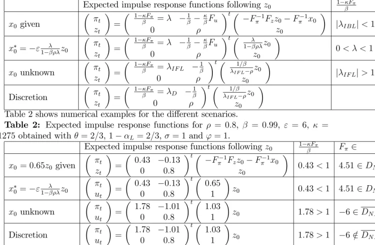
Table 2 shows numerical examples for the di¤erent scenarios.

Table 2: Expected impulse response functions for = 0:8, = 0:99, " = 6, =

0:1275 obtained with = 2=3, 1 L= 2=3, = 1 and ' = 1.

Expected impulse response functions following z0 1 F F 2 Fz

x0 = 0:65z0 given t zt = 0:43 0:13 0 0:8 t F 1Fzz0 F 1x0 z0 0:43 < 1 4:51 _{2 D}N F 6:83 x₀ = "₁ z0 t ut = 0:43 0:13 0 0:8 t 0:65 1 z0 0:43 < 1 4:51 2 DN F 6:83 x0 unknown _ut t = 1:78 1:01 0 0:8 t 1:03 1 z0 1:78 > 1 62 DN F 0 Discretion t ut = 1:78 1:01 0 0:8 t 1:03 1 z0 1:78 > 1 6 =2 DN F 0

Giordani and Söderlind (2006) demonstrated that the simple-rule solution with forward-looking policy instruments and forward-forward-looking policy targets does not satisfy robustness to misspeci…cation as de…ned by Hansen and Sargent (2008). The evil agent of robust control trying to fool the policy maker as much as he can is turned into the most helpful angel agent which tries to help as much as he can the policy maker to save his locally un-stable path in the space of policy target variables. Macroeconomists advise policy makers

that the local instability of the dynamics of the policy maker’s state variables is necessary in order to achieve macroeconomic stabilization. This solution is turning upside down the theories of classic, optimal and robust control and of Stackelberg dynamic games. Its policy recommendations have zero robustness and zero credibility (Cochrane (2019) p.345).

The uncertainty on the knowledge of parameters is strictly restricted, so that the local instability of the equilibrium in the space of n state variables of the solution with forward-looking hypothesis does not matter. A shock on one parameter is instantaneously o¤set by another shock on another parameter (by the virtue of the angel agent) so that the dynamics of the n state variables remains in a stable subset of dimension m < n.

In our example, assume that the policy rule F is chosen by the policy maker and the stable subspace projection parameter G anchoring in‡ation on the non-observable cost-push auto-regressive shock is chosen by the private sector.

t= Gzt and xt = F t with G =

1

1 F :

This solution remains stable only if the uncertainty on the parameters , and

satis…es this restriction:

= 1

F 1

G+ 1 :

A deviation of should be instantaneously compensated by a deviation of so

that G and F remain unchanged. There is the underlying assumption of a angel agent who creates an exact negative-feedback correlation between exogenous shocks. Hence, the local instability in the space of policy targets of dimension two does not change the stable dynamics of in‡ation and of the policy instrument in a subspace of dimension one. When , , vary in continuous intervals of real numbers, this restriction has a probability equal to zero. Robustness of misspeci…cation can also be ruled out by assuming the knowledge of all the parameters of the policy transmission mechanism with in…nite precision.

4

Conclusion

After having analyzed the di¤erent scenarios of forward or backward looking policy in-struments and their relation to the policy targets, we will propose two criteria for choosing the appropriate economic model. The …rst concerns the robustness of the model:

Criterion 1 A model of policy maker’s behavior should provide policy recommendations

which are robust to misspeci…cation when the policy maker is facing uncertainty on the values of the parameters of the economy. A necessary (but not su¢ cient) condition is to use negative-feedback policy rule parameters.

The second criterion concerns the way the central bank’s behavior is modeled. Sim-ple rules with proportional feedback as used in New-Keynesian DSCG models where a policy instrument responds to forward-looking policy targets does not imply that policy instruments are forward-looking variables. These models are sometimes considered to have better theoretical foundations due to optimal behavior with respect to agent-based models using behavioral simple rules. Consistency implies that this argument of the ra-tional micro-foundation of optimal choice should also apply to the policy maker. The

…rst best method is to abandon once and for all ambiguous simple-rule models and to shift to models of Ramsey optimal policy under quasi-commitment. If simple rules are still assumed as a second best theory, the outcome of their model should be as close as possible to Ramsey optimal policy under quasi-commitment.

Criterion 2 Simple-rule parameters should be reduced forms of the rules of Ramsey

op-timal policy under quasi-commitment, which would imply a minimal robustness to mis-speci…cation and a minimal credibility of stabilization policy.

As seen in the example, this criterion can be satis…ed with the backward-looking hypothesis for a range of values of the policy-rule parameters.

This paper suggest that new-Keynesian DSGE models and the …scal theory of the price level are currently locked in to the inferior technology path of having chosen the convention of forward-looking policy instrument if policy targets are forward-looking, as it happened for QWERTY typewriter keyboard with respect to DVORAK (David (1985)).

References

[1] Blanchard O.J. and Kahn C. (1980). The solution of linear di¤erence models under rational expectations. Econometrica , 48, 1305-1311.

[2] Chatelain J. B. and Ralf K. (2019). A Simple Algorithm for Solving Ramsey Optimal Policy with Exogenous Forcing Variables. Economics Bulletin, 39, 2429-2440. [3] Chatelain J. B. and Ralf K. (2018). Publish and Perish: Creative Destruction and

Macroeconomic Theory. History of Economic Ideas, 26, 65-101.

[4] Clarida R., Gali J. and Gertler M. (1999). The science of monetary policy: a new Keynesian perspective. Journal of Economic Literature, 37, 1661-1707.

[5] Cochrane, J. H. (2019). The Fiscal Theory of the Price Level. Manuscript. URL https://faculty. chicagobooth. edu/john. cochrane.

[6] Currie, D., & Levine, P. (1985). Macroeconomic policy design in an interdependent world. In: International Economic Policy Coordination. Cambridge University Press, 228-273.

[7] David P. A. (1985). Clio and the Economics of QWERTY. The American economic review, 75, 332-337.

[8] Gali J. (2015). Monetary Policy, In‡ation and the Business Cycle. 2nd. edition, Princeton University Press, Princeton.

[9] Giordani P. and Söderlind P. (2004). Solution of Macromodels with Hansen-Sargent Robust Policies: some extensions. Journal of Economic Dynamics and Control, 12, 2367-2397.

[10] Hansen L.P. and Sargent T. (2008). Robustness. Princeton University Press, Prince-ton.

[11] Kalman R.E. (1960). Contributions to the Theory of Optimal Control. Boletin de la Sociedad Matematica Mexicana, 5, 102-109.

[12] Kydland, F. E., & Prescott, E. C. (1980). Dynamic optimal taxation, rational expec-tations and optimal control. Journal of Economic Dynamics and control, 2, 79-91. [13] Leeper E. M. (1991). Equilibria under ‘active’ and ‘passive’ monetary and …scal

policies. Journal of Monetary Economics, 27, 129-147.

[14] Ljungqvist L. and Sargent T.J. (2012). Recursive Macroeconomic Theory. 3rd edition. The MIT Press. Cambridge, Massachusetts.

[15] Roberds W. (1987). Models of policy under stochastic replanning. International Eco-nomic Review, 28, 731-755.

[16] Schaumburg E. and Tambalotti A. (2007). An investigation of the gains from com-mitment in monetary policy. Journal of Monetary Economics, 54, 302-324.

[17] Vaughan D. (1970). A nonrecursive algebraic solution for the discrete Riccati equa-tion. IEEE Transactions on Automatic Control, 15, 597-599.

[18] Wonham W.N. (1967). On pole assignment in multi-input controllable linear system. IEEE transactions on Automatic Control. 12, 660-665.

[19] Woodford M. (2003). Interest and prices: Foundations of a theory of monetary policy. Princeton University Press, Princeton.