HAL Id: hal-03210014
https://hal.archives-ouvertes.fr/hal-03210014
Submitted on 30 Apr 2021
HAL is a multi-disciplinary open access
archive for the deposit and dissemination of sci-entific research documents, whether they are pub-lished or not. The documents may come from teaching and research institutions in France or
L’archive ouverte pluridisciplinaire HAL, est destinée au dépôt et à la diffusion de documents scientifiques de niveau recherche, publiés ou non, émanant des établissements d’enseignement et de recherche français ou étrangers, des laboratoires
Southern Hemisphere westerly wind changes during the
Last Glacial Maximum: model-data comparison
Louise Sime, Karen Kohfeld, Corinne Le Quéré, Eric Wolff, Agatha de Boer,
Robert Graham, Laurent Bopp
To cite this version:
Louise Sime, Karen Kohfeld, Corinne Le Quéré, Eric Wolff, Agatha de Boer, et al.. Southern Hemi-sphere westerly wind changes during the Last Glacial Maximum: model-data comparison. Quaternary Science Reviews, Elsevier, 2013, 64, pp.104-120. �10.1016/j.quascirev.2012.12.008�. �hal-03210014�
Southern Hemisphere Westerly Wind Changes during
the Last Glacial Maximum: Model-Data Comparison
Louise C. Simea, Karen E. Kohfeldb, Corinne Le Qu´er´ec, Eric W. Wolffa, Agatha M. de Boerd, Robert M. Grahamd, Laurent Boppe
aBritish Antarctic Survey, Cambridge, CB3 0ET, U.K.
bSimon Fraser University, 8888 University Drive, Burnaby, V5A 1S6, Canada
cSchool of Environmental Sciences, University of East Anglia, Norwich, NR4 7TJ, U.K
dDepartment of Geological Sciences, Stockholm University, 106 91 Stockholm, Sweden
eCentre National de la Recherche Scientifique, CEA, Saclay, 91191, France
Abstract
The Southern Hemisphere (SH) westerly winds are thought to be critical
1
to global ocean circulation, productivity, and carbon storage. For example,
2
an equatorward shift in the winds, though its affect on the Southern Ocean
3
circulation, has been suggested as the leading cause for the reduction in
at-4
mospheric CO2 during the last glacial period. Despite the importance of
5
the winds, it is currently not clear, from observations or model results, how
6
they behave during the last glacial. Here, an atmospheric modelling study
7
is performed to help determine likely changes in the SH westerly winds
dur-8
ing the Last Glacial Maximum (LGM). Using LGM boundary conditions,
9
the maximum in SH westerlies is strengthened by ∼ +1 ms−1 and moved
10
southward by∼2◦at the 850 hPa pressure level. Boundary layer stabilisation
11
effects over equatorward extended LGM sea-ice can lead to a small
appar-12
ent equatorward shift in the wind band at the surface. Further sensitivity
13
analysis with individual boundary condition changes indicate that changes
14
in sea surface temperatures are the strongest factor behind the wind change.
15
The HadAM3 atmospheric simulations, along with published PMIP2 coupled
16
climate model simulations, are then assessed against the newly synthesised
17
database of moisture observations for the LGM. Although the moisture data
18
is the most commonly cited evidence in support of a large equatorward shift
19
in the SH winds during the LGM, none of the models that produce realistic
20
LGM precipitation changes show such a large equatorward shift. In fact,
21
the model which best simulates the moisture proxy data is the HadAM3
22
LGM simulation which shows a small poleward wind shift. While we cannot
prove here that a large equatorward shift would not be able to reproduce the
24
moisture data as well, we show that the moisture proxies do not provide an
25
observational evidence base for it.
26
Keywords: glacial-interglacial cycles, westerly winds, Southern Ocean, LGM, atmospheric modelling, PMIP2, data-model comparison
1. Introduction
27
The location and the strength of Southern Hemisphere (SH) westerly
28
winds play a critical role in global climate, with glacial-interglacial change
29
in CO2 strongly linked to ocean-atmosphere circulation feedbacks mediated
30
through the SH wind field (Sigman and Boyle, 2000; Toggweiler et al., 2006;
31
Levermann et al., 2007; Toggweiler and Russell, 2008; Toggweiler, 2009;
Den-32
ton et al., 2010; De Boer et al., 2010). For example, oceanic carbon
seques-33
tration depends strongly on Southern Ocean circulation, which is influenced
34
by this wind field (Toggweiler, 1999; Wunsch, 2003; Le Qu´er´e et al., 2007;
35
Toggweiler and Russell, 2008). If glacial period equatorward positioned
west-36
erlies occurred, it is thought that they would curtail deep water ventilation
37
and lead to a more stratified ocean (Toggweiler and Samuels, 1995, 1998).
38
Isolated deep water traps carbon and leads to a reduction in atmospheric
39
CO2 (Toggweiler, 1999; Watson and Naveira Garabato, 2006; Skinner et al.,
40
2010; Sigman et al., 2010).
41
In addition to this primary ocean-CO2 modulation mechanism, other
po-42
tential oceanic impacts of wind changes have been identified. The impact of
43
SH winds on North Atlantic Deep Water (NADW) formation through
dy-44
namical processes has been established (Toggweiler and Samuels, 1993, 1995;
45
Rahmstorf and England, 1997; Nof and De Boer, 2004; De Boer and Nof,
46
2005; De Boer et al., 2008). Another hypothesis that has recently gained
47
prominence is the suggestion that SH westerly winds affect NADW
forma-48
tion though its modulation of Agulhas Leakage (Sijp and England, 2009; Beal
49
et al., 2011; Caley et al., 2012), the idea being that an equatorward shift in
50
the SH winds forces a similar shift in the Subtropical Front, in turn
reduc-51
ing the amount of high salinity Indian Ocean water that enters the Atlantic
52
Ocean. The decrease in Atlantic salt input then translates into a weaker
53
Atlantic meridional overturning.
54
Outwith the ocean, changes in the SH westerlies may also modify other
55
parts of the climate system that are critical to the ocean-atmospheric CO2
balance. For example, iron rich dust borne by SH winds affects Southern
57
Ocean productivity, thereby influencing the ocean-atmosphere carbon budget
58
(Kohfeld et al., 2005).
59
Given this critical importance of SH westerly winds for the ocean
circula-60
tion and climate, it is thus important that we both understand what controls
61
their changes and how we can read wind changes from paleo-enviromental
62
evidence.
63
Kohfeld et al. (submitted) discussed how the location and strength of
64
the westerly winds during the glacial period have been inferred using
recon-65
structed paleo-changes in moisture conditions and sometimes oceanic front
66
shifts (Bard and Rickaby, 2009; Kohfeld et al., submitted). Inferred changes
67
in precipitation reconstructed from vegetation regimes, lakes, glaciers, and
68
other precipitation sensitive paleo-environments have been interpreted as
69
equatorward shifts in the winds as large as 7-10◦ relative to their interglacial
70
position (Heusser, 1989; Lamy et al., 1999; Moreno et al., 1999; Toggweiler,
71
1999; Toggweiler et al., 2006; Toggweiler and Russell, 2008; Toggweiler, 2009).
72
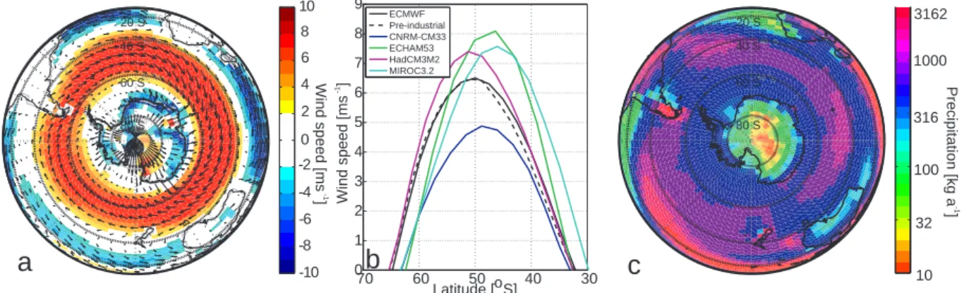
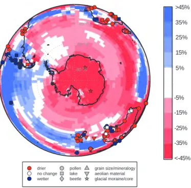
We note here that this interpretation has arisen from the relationship between
73
present-day SH westerlies and precipitation (Fig. 1ac). Thus, in places such
74
as South America, an equatorward shift in westerly winds during the last
75
glacial period has been inferred from data that demonstrate enhanced
pre-76
cipitation to the north of the modern-day position of the SH westerlies, and
77
colder drier conditions in more southerly locations (Heusser, 1989; Lamy
78
et al., 1999; Moreno et al., 1999). This proposed shift has often been
asso-79
ciated with a proposed glacial weakening of the Hadley cell (Williams and
80
Bryan, 2006; Toggweiler and Russell, 2008; Toggweiler, 2009; Denton et al.,
81
2010). See Kohfeld et al. (submitted) for additional details and other possible
82
interpretations of this data.
83
Model studies do not agree on the position and strength of the westerly
84
winds during the Last Glacial Maximum (LGM - 19-23 ky) conditions.
Stud-85
ies using coupled Atmosphere-Ocean General Circulation Models (AOGCM)
86
have suggested that the westerlies move equatorward (Williams and Bryan,
87
2006) and weaken (Kim et al., 2002, 2003); move poleward and strengthen
88
(Shin et al., 2003); move poleward (Kitoh et al., 2001); or increase in strength
89
with no latitudinal shift (Otto-Bliesner et al., 2006). Analysis of more recent
90
AOGCM Paleoclimate Modelling Intercomparison Project 2 (PMIP2) wind
91
results still shows similar variation between different models (Menviel et al.,
92
2008; Rojas et al., 2009). Likewise, studies using atmosphere-only General
93
Circulation Models (AGCMs) have shown both equatorward (Drost et al.,
2007) and poleward shifts (Wyrwoll et al., 2000).
95
This apparent disconnect between modelling results and paleo-observations
96
represents a serious gap in our knowledge about the nature of changes in
97
westerly winds, and our ability to understand the impacts of these changes.
98
This paper represents the second of two research contributions to examine
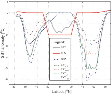
99
how westerly winds behaved during the LGM. In our first paper (Kohfeld
100
et al., submitted), we synthesize and summarise interpretations of
paleo-101
enviromental observations relating to the SH westerlies during the LGM. We
102
conclude that resolving the position and strength of the westerly winds based
103
on this data alone remains difficult because of several possible interpretations.
104
Kohfeld et al. (submitted) shows that that although atmospheric evidence
105
has been frequently used to support the hypothesised large equatorward shift
106
or strengthening, the assumptions used have not been tested previously.
107
Here, our goal is to make progress through modelling, and by an
atmo-108
spheric data-model intercomparison. To this purpose we perform a set of
109
atmospheric modelling experiments to simulate the glacial winds using LGM
110
boundary conditions. We further test the sensitivity of the winds to each
in-111
dividual LGM boundary condition change. In section 2 we lay out the design
112
of the atmospheric modelling experiments, note the PMIP2 AOGCM coupled
113
simulations to which we compare our results, and explain how we quantify
114
the comparison of model output with observations. In section 3, we explore
115
how SH westerly winds change in response to individual LGM boundary
con-116
dition changes. In section 4, we explore the SH moisture changes, comparing
117
HadAM3 AGCM and PMIP2 AOGCM moisture changes with the main
Ko-118
hfeld et al. (submitted) moisture observation synthesis. Implications of the
119
results are discussed within the context of observed dust and oceanic front
120
changes in section 5.
121
2. Experiment design
122
2.1. AGCM (HadAM3) model description
123
To test the sensitivity of SH winds and moisture to changes in
glacial-124
interglacial atmospheric boundary conditions, experiments are set-up using
125
an atmospheric-only model HadAM3 on a regular latitude longitude grid
126
with a horizontal resolution of 2.5 ◦× 3.75◦, and 20 hybrid coordinate levels
127
in the vertical (Pope et al., 2000). HadAM3 features a good representation of
128
present day model climatology (Pope et al., 2000). Where the model is run in
129
its coupled state (HadCM3), it features a reasonable representation (Fig 1b)
of the mean annual SH westerlies (Russell et al., 2006) and produces
realis-131
tic simulations of coupled wind dependent low frequency variability (Gordon
132
et al., 2000; Collins et al., 2001; Sime et al., 2006). This suggests that the
133
atmospheric response to sea surface temperature and sea-ice change is
re-134
liable. A pre-industrial control simulation is performed along with 9 LGM
135
sensitivity experiments.
136
2.2. Simulation boundary conditions
137
The prescribed boundary conditions for each model integration includes
138
values for sea surface temperature, sea-ice, land-ice, solar insolation, and
139
atmospheric gas concentrations.
140
The sea surface temperature and sea-ice data for our pre-industrial (PI)
141
control simulation are based on a twenty year monthly average of HadiSST
142
data (Rayner et al., 2003). Ice-sheet volume (and therefore also the land-sea
143
masking) and insolation conditions are taken from the present-day, but
at-144
mospheric gas composition is set to pre-industrial values (CO2 is 280 ppmv;
145
CH4 is 0.76 ppmv; and N2O is 0.27 ppmv). SH westerly winds in this
pre-146
industrial simulation (Fig. 1a) are close to the early period European Centre
147
for Medium-Range Weather Forecasts (ECMWF) zonal winds (Fig. 1b);
148
early period data are used to validate the model simulation to minimise the
149
effect of warming or ozone changes on the comparison (Shindell and Schmidt,
150
2004). Similarly, the pre-industrial precipitation, is also in reasonable
agree-151
ment with ECMWF precipitation. The comparison between ECMWF and
152
the control simulation suggests that the SH westerlies and the precipitation
153
regime in the HadAM3 pre-industrial experiment are reasonable in
compar-154
ison with coupled model results (Russell et al., 2006).
155
For the LGM, the most recent compilation of sea surface temperature data
156
is from the MARGO project MARGO Project Members (2009). We treat it
157
here as the best observational estimate available of glacial sea surface
condi-158
tions. However, at present, the MARGO compilation has not been
interpo-159
lated to produce a globally gridded dataset. A global dataset is required to
160
drive a global atmospheric general circulation model. The most recent
grid-161
ded version of the GLAMAP LGM (19-22 ky) sea surface conditions (Paul
162
and Sch¨afer-Neth, 2003a,b) is therefore used to drive the HadAM3
experi-163
ments (Fig. 2). Fig. 3a shows the difference between the gridded GLAMAP
164
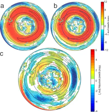
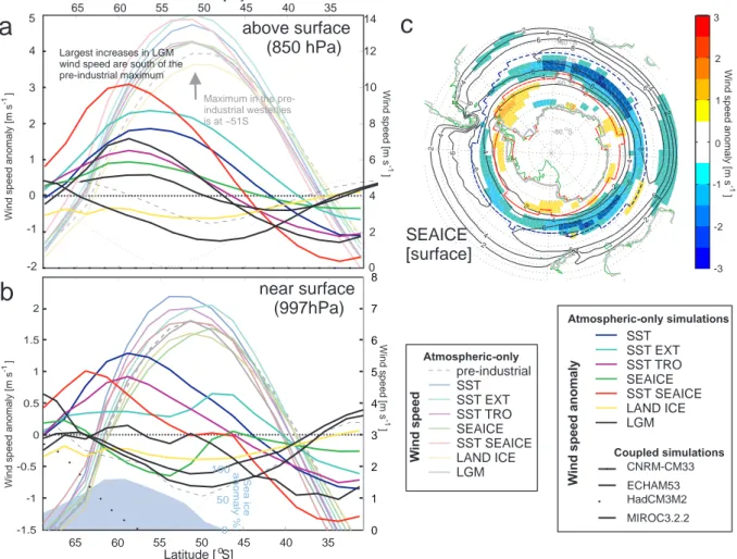
sea surface temperatures and sea-ice values and the MARGO data. The
165
GLAMAP LGM sea surface temperatures are mainly within 1-2 K of the
nearest MARGO values. However, some larger regional discrepancies
oc-167
cur, particularly around New Zealand, GLAMAP values here are generally
168
2-4 K too warm. The GLAMAP dataset is also used for our LGM sea-ice
169
conditions.
170
LGM sea surface temperature data is rather sparse poleward of 40◦S,
lead-171
ing to difficulty in establishing accurate meridional temperature gradients in
172
this region (MARGO Project Members, 2009). However, paleo-observations
173
of sea-ice extent allows estimation of the sea surface temperatures near the
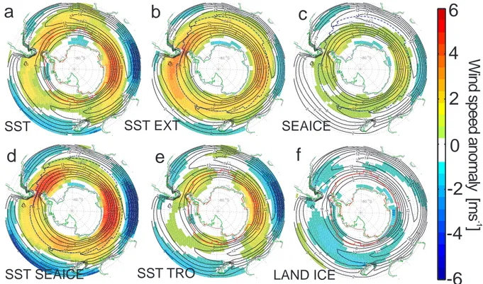
174
geographical LGM sea-ice limit (at about 55◦S), at roughly minus 2◦C
(Ger-175
sonde et al., 2005). Thus we have reasonable confidence that there was a
176
steeper LGM extra-tropical temperature gradient (Paul and Sch¨afer-Neth,
177
2003b). Compared with the polar regions, there are more glacial sea surface
178
temperature observations from the tropical regions (Paul and Sch¨afer-Neth,
179
2003b; MARGO Project Members, 2009). These extra observations improve
180
confidence in the tropical boundary conditions.
181
Orbitally dependent insolation for the LGM (Laskar et al., 2004) and
182
the atmospheric greenhouse gas composition (CO2 is 185 ppmv; CH4 is 0.35
183
ppmv; and N2O is 0.20 ppmv) is taken from the specified PMIP2
bound-184
ary conditions (Braconnot et al., 2007)) and are known relatively well.
Al-185
though there is uncertainty about detailed aspects of the East Antarctic
186
glacial ice-sheet morphology, we have used the broad-scale glacial-interglacial
187
ICE-5G(VM2) model mass changes in which there is reasonable confidence
188
(Peltier, 2004).
189
2.3. AGCM (HadAM3) sensitivity simulations
190
In addition to the PI control simulation,nine atmospheric-only GCM
sim-191
ulations are used to assess the LGM SH wind and moisture changes. The
192
most realistic LGM experiment, named LGM, applies all the known boundary
193
conditions for that period as described in the previous section. The
individ-194
ual sensitivity experiments are designed to simulate the effect of the various
195
observed LGM changes in sea surface temperatures, sea-ice, ice-sheets,
in-196
coming solar radiation, and atmospheric gas composition. The experiments
197
are generated by varying one boundary condition at a time from the PI to
198
the LGM conditions (Table 1). The atmospheric simulations are run for
199
30 years, which is long enough to allow the atmosphere to reach an
equi-200
librium state with the specified boundary conditions (for atmospheric-only
201
simulations, an equilibrium state is reached after approximately two to four
weeks). Results are presented as differences between pre-industrial and the
203
LGM-based simulations.
204
The details of the sensitivity experiments are as follows. The SST
exper-205
iment is identical to PI except using LGM sea surface temperature values.
206
The SEAICE experiment is identical to PI, except that LGM sea-ice
con-207
ditions are applied, i.e. this experiment uses LGM sea-ice-conditions, but
208
pre-industrial sea surface temperatures. This means that in the experiment
209
SEAICE sea-ice is prescribed in some areas where the surface temperature
210
is above −1.8◦C. The individual SST and SEAICE experiments are not
in-211
tended to represent realistic simulations of past conditions, but are useful
212
as they allow us to investigate separately the boundary condition effect of
213
sea surface temperature and sea-ice changes. SST SEAICE is more realistic
214
since it combines the sea surface temperature and sea-ice conditions from
215
the SST and SEAICE experiments. The TRO and EXT experiments are
216
variations of the SST SEAICE experiments. SST TRO is based on PI but
217
has the LGM GLAMAP reconstruction imposed equatorward of 20◦ with a
218
linear reduction in the anomaly imposed between 20◦ and 30◦: poleward of
219
30◦ SST TRO is identical to PI. Similarly, SST EXT has the GLAMAP sea
220
surface reconstruction imposed between 90◦ and 30◦, with a linear reduction
221
to zero between 30◦ and 20◦, and PI conditions equatorward of 20◦. LAND
222
ICE ice-sheet volume, ice-sheet topography, and land-sea masking is adjusted
223
to LGM conditions. ORBIT varies from the PI experiment in orbital
param-224
eters. GAS uses LGM atmospheric gas composition values. The HadAM3
225
LGM experiment combines all the different LGM changes.
226
To help examine the impact of uncertainties in the sea surface
temper-227
ature observations, twelve additional sensitivity simulations were also
per-228
formed. See Appendix A for these additional experiments.
229
2.4. Description of AOGCM (PMIP2) simulations
230
To assess the robustness of the results from the AGCM HadAM3
ex-231
periments, the published AOGCM PMIP2 simulations are also analysed
232
where surface and 850 HPa wind and precipitation fields are available. The
233
AOGCM pre-industrial simulations are similar in specification to the full
234
LGM AGCM simulation, except that they are run with a full dynamic ocean
235
and sea-ice model, rather than with specified sea surface conditions (Table 1).
236
The simulations are run for long enough to allow the atmosphere and oceans
237
reach quasi-equilibrium state to the specified boundary conditions and for
trends to become small (Rojas et al., 2009). In these ocean-atmosphere
sim-239
ulations, the pre-industrial SH westerlies band is less well simulated compared
240
to our atmospheric-only simulation, with a general bias towards westerlies
241
that are too intense and located too far north (Fig. 1b). These pre-industrial
242
simulation errors hinder comparison with the glacial simulation winds. This
243
difficulty can cloud the picture of interglacial to glacial wind changes obtained
244
from AOGCM simulations (Rojas et al. 2009). However, their atmosphere,
245
ocean, and sea-ice components are dynamically consistent with each other
246
(Rojas et al., 2009) and analysis of these coupled simulations sheds light on
247
the sensitivity of our results to model choice.
248
Analysing coupled AOGCM LGM multi-model simulations, alongside
249
core AGCM simulations, ensures that a wide possible range of LGM model
250
results are considered. The comparison between MARGO sea surface
tem-251
perature data and the two PMIP2 simulations, for which we have the
com-252
parative sea surface temperature output, suggests that as we might expect
253
the LGM sea surface conditions are slightly better represented by the
obser-254
vationally based GLAMAP AGCM boundary condition data, compared to
255
the AOGCM simulations (Fig. 3). Some problems in the accuracy of
sim-256
ulated LGM sea surface conditions from coupled atmospheric-ocean models
257
may be due to difficulties in accurately parameterising glacial ocean mixing
258
terms (Wunsch, 2003; Watson and Naveira Garabato, 2006), and also partly a
259
problem of model resolution. Both of these problems affect the simulation of
260
the narrow Southern Ocean frontal jets which dominate the Southern Ocean
261
surface temperature patterns. Further improvements in ocean model
param-262
eterisation, and also in model resolution, may in future help to resolve these
263
glacial ocean simulation problems. These type of ocean modelling problems
264
also afflict coupled PMIP2 pre-industrial simulations (Russell et al., 2006),
265
thus errors in the pre-industrial ocean surface temperature simulation may
266
be the cause of errors in the simulated pre-industrial SH westerly winds (Fig.
267
1b).
268
2.5. Data-model comparison metrics
269
The Kohfeld et al. (submitted) paleo-observational study compiles
evi-270
dence of widespread glacial-interglacial moisture changes in the SH.
Simula-271
tion results are evaluated against 105 observations from 97 locations in this
272
new synthesized moisture dataset, by visual inspection and using two
quan-273
titative approaches.The first quantitative approach compares simulated and
274
observed changes at the ‘exact’ observation location, whilst the second checks
for a ‘local’ match. The local-match approach helps allow for model-inability
276
to represent small scale topographic features that are not represented in
277
GCMs but may affect observations. Both model evaluation techniques allow
278
the use of simple percentage statistics (Tables 1-3). This independent
evalu-279
ation of the goodness of model simulations helps in allowing investigation of
280
both glacial-interglacial SH circulation and moisture changes.
281
The assessment of the exact-type and local-type agreement between
mod-282
elled and observed moisture matches is made by classing simulated
precip-283
itation changes as positive or negative, if they are larger than ±5 %. This
284
5% threshold allows for a total 10% to be attributable to uncertainty in the
285
interpretation of proxies, or simulation of the changes. A simulated change
286
of less than 5 % is classified as no change. This threshold is narrow compared
287
to discussion on pollen-proxy sensitivity (Bartlein et al., 2011), however
re-288
cent evaluations of model simulations against paleo-data have shown that
289
models tend to underestimate the magnitude of precipitation changes,
par-290
ticularly regional changes (Braconnot et al., 2012). Our result here support
291
the Braconnot et al. (2012) finding: the 5% threshold gives a better match
292
with paleo-data compared with using a wider ±10 % threshold (not shown).
293
In the exact-type approach, simulation change values are linearly
inter-294
polated to the exact observation site before the threshold is applied. The
295
number of sites which match the observed changes can then be presented as
296
simple percentage statistic, i.e. if 20 of 100 observations match, then the
sim-297
ulation scores 20% (Table 1). For a local-type approach, simulation changes
298
are calculated as above (using the same threshold), but rather than
interpo-299
late directly to the observation site, the simulation results (on the original
300
model grid) are searched within a given radius for a locally correct match
301
(Table 1, last column). This local approach helps allow for model inability
302
to represent localised effects of gradients on moisture: small-scale features
303
affect observations but relatively coarse resolution models cannot simulate
304
them. Even given the local-type method, it is unlikely that any relatively
305
coarse resolution model study will achieve a perfect observation match.
306
The local-type percentage agreements are checked using a variety of
spa-307
tial search radiuses. The main local-type match results given in Table 1 use
308
a radius of 400 km. This radius is used because it matches the approximate
309
resolution of the model grid at the equator (3.75◦distance in longitude at
310
0◦ latitude is 417 km). However, as one moves towards the poles this
dis-311
tances decreases (e.g. it is 341 km at 35◦S, 295 km at 45◦S, 268 km at 50◦S,
312
and so on). Largely because of this variation, it is not possible to choose
a search radius where the ’local’ and ’exact’ model-observation agreement
314
results are in perfect agreement. However, in general, reducing the radius
315
towards about 250 km brings these results into rough agreement, since that
316
means that usually about one model grid point is within the local search
317
radius. We also present metrics in Table 2 and 3 using these alternative
318
search radii. It can be argued that data-model metrics for the extra-tropical
319
region, from 35◦S to 90◦S are the more relevant for understanding Southern
320
Ocean westerly wind changes. We therefore also provide results for separate
321
tropical (0-35◦S) and extra-tropical (35-90◦S) sub-domains in Tables 2 and
322
3, and compare these results to those for the whole SH domain.
323
Due to the three-value nature of our results (wetter, drier, or no change)
324
we cannot apply common statistical tests to the datasets. However, by
ran-325
domising the relationship between the given observations against simulation
326
results, we can calculate null agreement values for the simulations. Assuming
327
the simulation of equal areas or wetter, drier, and no change in precipitation,
328
the exact-type null value is 33%, and the local-type null value is 57% for a
329
400 km radius, and 44% for 250 km. Thus percentage values higher than
330
these numbers indicate skill in the model simulation. Note whilst local-type
331
null values vary slightly between simulations (due to the variable
geograph-332
ical pattern of changes), using the ECHAM5, MIROC3.2.2, and HadCM3
333
AOGCM LGM simulation, null results are within two percentage points of
334
each other.
335
Moisture observations tend to reflect moisture flux (i.e. P-E). However,
336
for HadAM3 simulations, the precipitation and moisture flux
observation-337
model local-type match comparisons are quite similar: within 10% of each
338
other for simulations that do not involve ICE-5G; and with a maximum
dif-339
ference of 12% for simulations using ICE-5G. Since we do not have PMIP2
340
moisture flux fields available, observations are tested against simulation
pre-341
cipitation changes for both HadAM3 and coupled PMIP2 simulations (Table
342
1, right columns).
343
3. Simulated changes in LGM winds
344
In our atmospheric LGM simulation full glacial boundary conditions are
345
imposed and the results compared to the pre-industrial control. For this
346
simulation, the 850 hPa westerlies show a small increase poleward of 50◦S
347
(+1.5 ms−1 at 60◦S) and a small decrease northward of 50◦S (−1 ms−1 at
348
40◦S) leading to a maximum that is shifted poleward by about 2◦ (Fig. 4).
At 2◦ the latitudinal shift of the 850 hPa wind band obtained here is rather
350
small and in the opposite direction from what has often been suggested
(Tog-351
gweiler et al., 2006; Toggweiler and Russell, 2008; Toggweiler, 2009). In the
352
core region of the westerlies, at about 52◦S, the maximum increases by
ap-353
proximately +1 ms−1. We concentrate here on wind changes at 850 hPa
354
level, which are similar to those at the surface but do not include boundary
355
layer effects due to sea-ice cover. Surface wind effects and moisture changes
356
are considered in the later sections. Our sensitivity experiments (Table 1)
357
allow the effect of various LGM boundary conditions to be compared to their
358
individual impact on the atmospheric circulation (Fig. 5). The experiments
359
are used to examine LGM changes in the westerlies due to: [1] extra-tropical
360
and tropical sea surface conditions; and [2] orbitally dependent insolation,
361
atmospheric gases, and the morphology of the Antarctic ice-sheet.
362
3.1. The role of sea surface changes
363
In the SST EXT simulation where tropical sea surface temperatures are
364
held at pre-industrial levels and glacial sea surface temperatures are imposed
365
poleward of 20◦, a small ∼1◦ poleward shift in the location of the winds
366
maximum occurs. Pronounced cooling near the edge of the LGM Southern
367
Ocean sea-ice (Fig. 5ab) and extended sea-ice coverage (Fig. 5c) drives a
368
small intensification of the westerlies. The wind intensification is largest
be-369
tween 56-58◦S; approximately 5◦poleward of the pre-industrial maximum in
370
the winds location (Fig. 6a). This pattern of change drives the small
pole-371
ward shift in the location of the winds maximum. Observational evidence for
372
extended Antarctic sea-ice (Gersonde et al., 2005), supports an increase in
373
the glacial meridional temperature gradient around 55◦S. This steeper
South-374
ern Ocean surface meridional temperature gradient (Paul and Sch¨afer-Neth,
375
2003b; Gersonde et al., 2005), is associated with increased available
poten-376
tial energy (Wyrwoll et al., 2000; Wunsch, 2003), and increased potential
377
atmospheric baroclinicity. Similar intensifications in the westerlies, due to
378
southern cooling, are visible in the poleward intensifications of westerlies in
379
some previous studies (Wyrwoll et al., 2000; Yin and Battisti, 2001; Kitoh
380
et al., 2001).
381
In the SST TRO tropical simulations, sea surface temperatures
equa-382
torward of 20◦are set to glacial values, while Southern Ocean sea surface
383
temperatures are set at pre-industrial values. In contrast to local
temper-384
ature gradient effects discussed above, the tropical sea surface temperature
385
changes affect atmospheric temperature gradients in regions distant from
the band of SH westerlies. Reduced tropical sea surface temperatures cause
387
pressure changes through modifications of the Rossby wave pattern
(Lachlan-388
Cope et al., 2007), particularly in the SH wavenumber-3 pattern (Marshall
389
and Connolley, 2006). This leads to geographical variability in wind changes
390
around the Southern Ocean (Yin and Battisti, 2001). The Indian Ocean
391
sector experiences the largest changes, but every ocean basin sector sees an
392
intensification of the glacial westerlies south of 50◦S and a reduction to the
393
north (Fig. 5de). This leads to a small∼1◦poleward shift in the location of
394
the winds maximum (Fig. 6a).
395
The detail of the glacial tropical sea surface temperatures is still a matter
396
of ongoing research (MARGO Project Members, 2009), however analysis of
397
additional sensitivity experiments (Appendix A) confirms that this small
398
poleward shift in the SH westerlies appears to be a robust response to tropical
399
cooling. Note a much larger uniform −4K tropical cooling causes a very
400
similar, but intensified, pattern of wind changes (not shown).
401
3.2. The roles of orbit, greenhouse gases, and ice volume
402
In the orbital forcing and greenhouse gas simulations, these boundary
403
conditions are changed to glacial values, whilst all other conditions are kept
404
pre-industrial. The direct forcing of glacial-interglacial changes in orbital
405
parameters and atmospheric gas composition on atmospheric circulation is
406
small. Our results confirm that orbital changes do not lead to substantial
407
changes between the pre-industrial and the LGM westerlies, whilst
green-408
house gas changes lead to small reductions in the strength of the average
409
westerlies (of 0.25-0.5 ms−1). These glacial boundary conditions only cause
410
larger changes in the westerlies in ocean-atmosphere coupled GCMs where
411
sea surface temperature and sea-ice feedbacks may amplify initial forcings
412
(Rojas et al., 2009).
413
In the glacial ice volume simulation, glacial ice-sheets are imposed (Peltier,
414
2004), whilst other boundary conditions are kept pre-industrial. The changes,
415
in continents other than Antarctica, have little effect on hemispheric scale
416
wind patterns. However, the intensity of the westerlies south of 40◦S
de-417
creases according to the prescribed size of the Antarctic ice-sheet (Fig. 5f
418
and 6ab, yellow line). Katabatic winds drain out from the Antarctic
con-419
tinental ice-sheet, causing northerly and weak easterly surface flows around
420
the edge of the Antarctica (Fig. 1a, vectors). The higher ICE-5G (Peltier,
421
2004) LGM Antarctic ice-sheet results in steeper ice-sheet margin slopes,
422
with resultant increases in the strength of the katabatic winds (Heinemann,
2003). These more intense katabatic winds reduce the southward penetration
424
of cyclones (Parish et al., 1994), which reduces the average intensity of the
425
westerlies (Fig. 5f).
426
The Antarctic glacial ice volume increase (Peltier, 2004), together with
427
the extra-tropical surface temperature effects, reduce the simulated East
428
Antarctic Plateau LGM precipitation by approximately 70% (Fig. 7). This
429
reduction is larger than the observed decrease of about 50% (Parrenin et al.,
430
2007), and supports independent gas pressure evidence that the East
Antarc-431
tic ICE-5G ice-sheet elevation is probably too high (Masson-Delmotte et al.,
432
2006). In this case, our simulations using the ICE-5G ice reconstruction
433
may produce poleward westerly winds that are too weak; our Fig 6ab results
434
suggest somewhere from 0.2-0.5 ms−1 too weak.
435
3.3. The impact of wind prognostic choice
436
One factor which has affected comparison of previous glacial-interglacial
437
modelling studies is the choice of wind prognostic. Studies of SH
circu-438
lation change have used: surface winds (Kim et al., 2003); above-surface
439
winds; or surface shear stress (Otto-Bliesner et al., 2006). Where sea-ice
re-440
places pre-industrial open water, each of these prognostics shows a different
441
response. The intensity of surface winds is sensitive to the sea-ice extent
442
because expanded sea-ice cover leads to weak turbulent fluxes, strong
sta-443
ble stratification of the air layer above, and weaker surface winds (Fig. 5c
444
and 6c). Conversely, turbulent fluxes over the open ocean, or water with a
445
high fraction of leads, acts to intensify the surface winds (Heinemann, 2003).
446
Boundary layer sea-ice effects are also visible in some other model studies
447
which show a substantial weakening of the surface westerlies at high latitudes
448
(Kim et al., 2003). Outside the sea-ice zone, glacial-interglacial changes in
449
all atmospheric boundary conditions have a very similar impact on surface
450
and 850 hPa winds (Fig. 6ab). Whilst prognostic choice will depend on
sci-451
entific purpose, the above surface (around 850-hPa) winds may be the most
452
consistent prognostic between models for glacial-interglacial studies of the
453
SH westerlies because they do not suffer from boundary layer effects.
454
3.4. The impact of errors in the simulation of Southern Ocean sea surface
455
temperatures
456
A second factor, affecting coupled glacial-interglacial modelling studies is
457
errors in simulated pre-industrial Southern Ocean sea surface temperature
458
gradients. This leads to difficulty in interpreting some PMIP2 changes. For
example, the PMIP2-HadCM3M2 atmosphere-ocean simulation does not
fea-460
ture an enhanced glacial meridional temperature gradient and wind increases
461
in this region (Rojas et al., 2009; Drost et al., 2007). However, this is largely
462
due to overly strong temperature gradients and SH westerlies in the control
463
pre-industrial simulation (Fig. 1b). Some caution is therefore required in the
464
interpretation of Southern Ocean temperature gradient driven wind changes
465
in these coupled AOGCM simulations.
466
4. Simulated and observed moisture changes
467
Evaluating model results against the moisture observations offer a unique
468
means to assess the veracity of the simulated glacial-interglacial SH
circu-469
lation changes (Fig. 7-10). Examination of the the wind and
precipita-470
tion changes shows that the proposed glacial weakening of the Hadley cell
471
(Williams and Bryan, 2006; Toggweiler and Russell, 2008) occurs in several
472
of the LGM simulations, including the HadAM3 LGM simulation. Glacial
473
easterly winds weaken around 20◦S in each ocean basin (Fig. 4), and LGM
474
precipitation increases on the west side of South America and South Africa
475
south of 20◦S (Fig. 7). The reduced Hadley cell strength leads to reduced
476
subsidence related drying around 30◦S. However, contrary to what has been
477
suggested, the weakening of the Hadley cell does not lead to a significant
478
equatorward shift (Toggweiler, 2009; Denton et al., 2010) or to a weakening
479
(Williams and Bryan, 2006; Toggweiler and Russell, 2008) of the westerlies.
480
4.1. Interpreting Western Seaboard and wider SH LGM moisture changes
481
The local-type match between the annual mean atmospheric-only LGM
482
simulation and observed moisture changes is 100% on the west of all SH
con-483
tinents. This is important because most paleo-observational interpretations
484
which support a northward shift in the SH westerlies come from western
sea-485
board observations, between these latitudes (Kohfeld et al., submitted). If
486
we more simply restrict the spatial domain to between 35 and 90◦S (Table 2),
487
the match is 97%. An excellent model-observation match in these regions,
488
without a significant change in winds, provides a strong counter-argument
489
to the hypothesis that an equatorward shift in winds is required to explain
490
these observations.
491
The general pattern of moisture changes can be described thus. Due to
492
the extended sea-ice and Southern Ocean cooling, the extra-tropical
atmo-493
sphere cools and reduces the moisture holding capacity of atmosphere above
the Southern ocean (Fig. 9ac). This extra-tropical drying poleward of 50◦S
495
occurs in the AGCM and AOGCM LGM simulations (Fig. 7 and 10).
Equa-496
torwards, distinct regional patterns emerge from both the observational and
497
model analysis: sites between 30◦S and 45◦S in western South America all
498
experienced wetter conditions at the LGM compared to pre-industrial
con-499
ditions, due to reduced dry air subsidence (Fig. 9d). Sites south of 45◦S are
500
drier than pre-industrial conditions due to general atmospheric cooling and a
501
reduced moisture retaining capacity (Fig. 9ac 10). In addition to some
dry-502
ing on the central to east regions of the tip South America and Africa, there
503
is also some moistening on the south-west tips of Africa and New Zealand, in
504
both the simulations and in the paleo observations, some of which is related
505
to glacial-ice volume changes (Fig. 9b).
506
The exact-local type match analysis shows that the atmospheric-only
507
LGM simulation captures 57-83% of the moisture change observations. The
508
remaining unmatched 17% of moisture change paleo-observations include
ge-509
ographically closely spaced observations (of various signs) at about 5◦S in the
510
east of Africa, at 20◦S on the east coast of South America, and a few from
511
central southern region of Australia. These unmatched observations, from
512
the east or central tropical continental regions, may relate to uncertainties in
513
the tropical zonal gradient changes in our imposed sea surface temperatures
514
(MARGO Project Members, 2009). However, since simply imposing a
uni-515
form tropical cooling gives a relatively similar SH westerlies change pattern
516
(Appendix A), it is unlikely that plausible gradient errors could induce a
517
completely different simulated pattern of LGM SH westerlies.
518
4.2. Seasonal moisture and precipitation changes
519
Some moisture proxies, such as paleo-vegetation reconstructed from pollen,
520
are likely to reflect seasonal conditions (e.g. Heusser, 1990; Pickett et al.,
521
2004; Williams et al., 2009; Bartlein et al., 2011). Precipitation patterns
522
in parts of the Southern Hemisphere are distinctly seasonal in nature, and
523
the season reflected in the vegetation depends on the region examined (e.g.
524
Williams et al., 2009). Summer precipitation is influenced by southeast trade
525
winds (Gasse and Williamson, 2008; Zech et al., 2009) or the migration of
526
the Intertropical Convergence Zone near the equator (e.g. Barker and Gasse,
527
2003; Williams et al., 2009), and winter precipitation can be influenced by
528
winter migrations of the modern westerly winds (e.g. Gasse and Williamson,
529
2008; Lamy et al., 1999; Williams et al., 2009). Thus, it is valid to ask
whether the LGM moisture patterns inferred from paleo-data could
there-531
fore be mainly driven by one particular season, such as wintertime changes
532
influenced by the westerly wind band.
533
The HadAM3 LGM simulation provides a means to explore which
sea-534
sonal changes in precipitation patterns contribute to the observed changes in
535
our paleo-moisture reconstruction.
536
There are distinct changes to the precipitation patterns that persist
through-537
out the year (Fig. 8). However, there are also some seasonal changes. In
538
zones influenced by the modern-day westerlies band, all seasons show
en-539
hanced precipitation along the west coasts of South America and Africa
dur-540
ing the LGM, but the latitudes of enhanced precipitation can depend on
541
season. The overall effect is that the mean annual conditions show higher
542
precipitation all along the west coasts of these continents during the LGM,
543
and thus provide a better match to the data than individual seasons. In
con-544
trast, the simulated LGM increases in precipitation off southern Australia
545
and southern New Zealand are more seasonal, occurring predominantly in
546
austral autumn and winter. In this case, the increased winter precipitation
547
is not enough to offset the strength of the summer drying in the model. This
548
could decrease the coherence between the simulated mean annual
precipita-549
tion and observations.
550
Overall we find that the simulated mean annual conditions provide a
551
better match to the paleo-proxy data than simulated conditions for any
par-552
ticular season. It is possible that this is because the spatial extent of our
553
comparison covers regions in which different seasonal precipitation regimes
554
dominate, and the simulated mean annual precipitation is best able to
in-555
tegrate the net changes seen in all of these regions. When the exact match
556
model-data agreement metrics are calculated for these individual seasons we
557
find that the match is: 57% for the annual mean; 57% for the austral summer
558
(DJF); 55% for the austral autumn (MAM); 30% for austral winter (JJA);
559
and 47% for austral spring (SON) (see also Fig. 7). This suggests that it will
560
usually be more robust to use mean annual, rather than any individual
sin-561
gle season, results when testing LGM model simulations against the Kohfeld
562
et al. (submitted) moisture database. Finally, we note that given the
ocean-563
wind carbon hypothesis is constructed in terms of mean annual wind changes,
564
it is perhaps reassuring that the model-data match to the glacial-interglacial
565
moisture reconstruction is highest for mean annual conditions.
4.3. Hadley Cell induced changes
567
The sub-tropical moistening across each continent is related to the
tropi-568
cal sea surface changes (Fig. 9d), and an associated weakening of the Hadley
569
cell strength. Fig. 9-10, alongside Table 1 and Appendices A, show that
570
simulations which feature the weakening of the Hadley cell strength, tend to
571
have the strongest model-observation agreements. None of the simulations
572
which feature this change in the Hadley Cell strength feature a significant
573
equatorwards shift in the LGM SH westerlies.
574
Results from coupled ocean-atmosphere glacial PMIP2 simulations (Table
575
1) indicate that two AOGCMs, HadCM3M2 and MIROC3.2.2, also have
576
good matches of at least 53-70% (exact-local) to observed glacial-interglacial
577
moisture change. In common with the atmospheric only simulations, the
578
Hadley cell weakens in these simulations. Two other AOGCM simulations
579
feature lower model-observational scores of 44-63% (exact-local) and show
580
little or no reduction in Hadley cell strength. These less good matches to
581
observations suggest that these atmospheric simulations are less likely correct
582
in the SH. This PMIP2 data-model comparison supports the idea that that
583
the glacial Hadley cell was reduced in strength, but that the reduction was
584
not associated with a large (greater than 2◦) latitudinal shift in the position
585
of the westerly wind band.
586
5. Discussion of relation of results to a wider set of paleo-environmental
587
evidence
588
The section above indicates that LGM moisture changes, which comprise
589
the bulk of the available LGM Southern Hemisphere paleo-enviromental
at-590
mospheric change evidence (Kohfeld et al., submitted), can be explained
591
without a strengthening of westerly winds, except over the southerly areas
592
of the Southern Ocean. However, Kohfeld et al. (submitted) also discusses
593
and compiles other types of data which indicate LGM paleo-enviromental
594
changes. Whilst many of these observed changes were found to be too
diffi-595
cult to interpret as evidence which might support any wind change
hypoth-596
esis, here we nevertheless briefly discuss the implications of dust and ocean
597
front evidence in the context of our simulated LGM Southern Hemisphere
598
wind and moisture changes.
5.1. Observed LGM dust changes
600
One piece of paleo-enviromental evidence which has previously
inter-601
preted in terms of wind changes, is the enhanced dust fluxes to the ocean
602
surface and Antarctic continent during the LGM. Several factors could
con-603
tribute to greater dust: expanded source areas, reduced entrainment
thresh-604
olds (due to moisture reductions), stronger winds over these source regions,
605
greater residence times of dust, and increased transport lengths (due to
in-606
creased wind strengths). Although using a dust cycle model is beyond the
607
scope of this work, the LGM simulation shows drying in the areas we
as-608
sociate with LGM dust entrainment (Patagonia and shelf areas; Australia,
609
southern Africa; Fig. 7). Furthermore, stronger winds in the modern-day
610
Antarctic Circumpolar Current region and a drier atmosphere over much of
611
the Antarctic region (Fig. 4c and Fig. 7) suggest that the transport lengths,
612
and atmospheric residence time for dust, may have increased facilitating
613
greater amounts of dust transport to the Southern Ocean and Antarctica.
614
In addition, a lower LGM sea-level exposed more continental shelf, which
615
would have increased the potential dust source region size. Thus it is
possi-616
ble that the LGM atmospheric changes simulated here are in agreement with
617
observed LGM dust flux changes.
618
5.2. Observed ocean front changes: The Southern Ocean and the Agulhus
619
Current
620
On the position of Southern Ocean fronts, previous studies have argued
621
that equatorward shifts in these fronts may indicate an equatorward shift
622
of the westerly winds at the LGM (Howard and Prell, 1992; Kohfeld et al.,
623
submitted). This question cannot be addressed using our atmospheric
sim-624
ulations since the HadAM3 model use ocean surface conditions as an input.
625
The PMIP2 coupled simulations are also incapable of addressing this
ques-626
tion because their oceanic model components have a resolution too coarse
627
to resolve individual oceanic fronts. However, as a general comment on this,
628
Kohfeld et al. (submitted) both shows that the position of these fronts at the
629
LGM is presently under constrained in most sectors of the Southern Ocean,
630
and suggests that the nature of the relationship between winds and fronts is
631
also quite poorly understood.
632
Available paleo-evidence for the strength of the Southern Ocean Antarctic
633
Circumpolar Current (ACC) suggest that during the LGM it could either be
634
stronger than today (Noble et al., 2012) or of similar intensity (McCave
635
and Kuhn, 2012). If the ACC was a wind-driven current the observations
also indicate similar or stronger SH westerlies. However, this interpretation
637
is too simplistic because the ACC is now thought to be driven by both
638
buoyancy and wind forcing (Hogg, 2010; Allison et al., 2010; Munday et al.,
639
2011) . Recent oceanic modelling has also shown that significant changes in
640
ACC transport occur when diapycnal mixing changes in far-field sites ocean
641
basin (Munday et al., 2011), and such mixing changes have been proposed
642
for the LGM in response to sea level lowering (Wunsch, 2003). Thus, it is
643
probably not currently possible to draw any useful conclusion about whether
644
our simulated winds are in agreement with the LGM ACC strength.
645
We also note that LGM changes in Southern Ocean water masses and
646
ocean productivity cannot easily be interpreted in terms of wind changes
647
(Kohfeld et al., submitted).
648
Outside the Southern Ocean, a number of studies have indicated that
649
the volume of Agulhas Leakage was probably reduced during glacial periods
650
(Flores et al., 1999, 2003). It has been hypothesized that this is due to an
651
equatorward shift of the westerly wind belt and Subtropical Front (Bard and
652
Rickaby, 2009). However, a reduction in Agulhas Leakage may also be caused
653
by increased wind stress at the southern tip of South Africa, increasing the
654
wind stress curl over the subtropical gyre circulation in the Indian Basin
655
(Beal et al., 2011). Consistent with this particular hypothesis, our LGM
656
simulation shows increased wind speeds over this region.
657
6. Conclusions and implications for glacial winds
658
Whilst Southern Hemisphere (SH) westerly winds are thought to be
crit-659
ical to global ocean circulation, productivity, and carbon storage, it is
cur-660
rently not clear, from observations or model results, how they behave during
661
the last glacial (Kohfeld et al., submitted). Here we performed a set of
at-662
mospheric model simulations, including sensitivity simulations to examine
663
the impact of individual LGM boundary condition changes. We examined
664
the Southern Hemisphere westerly wind changes which occur as a result of
665
these boundary changes. Additionally, we compare both these simulations,
666
and PMIP2 coupled AOGCM simulations, with the new Kohfeld et al.
(sub-667
mitted) synthesised moisture database.
668
In our main atmospheric-only LGM simulation, the SH westerlies are
669
strengthened by ∼ +1 ms−1 and moved southward by ∼2◦at the 850 hPa
670
pressure level. However, boundary layer stabilisation effects over
equator-671
ward extended LGM sea-ice can lead to a small apparent equatorward shift
in the wind band at the surface. It is likely that this boundary layer effect,
673
due to extended LGM sea-ice, is one reason why some previous model studies
674
have suggested an equatorward shift in SH westerly winds. Thus the impact
675
of the choice of wind prognostic can lead to a divergence in the the apparent
676
SH westerly wind changes.
677
Interestingly, we find here that a reduction in Hadley Cell strength does
678
not equate to an equatorward shift of the westerlies. However, the weakening
679
does result in a wetting of the usually dry subsidence regions, which we
680
find can explain most of the observed LGM SH moisture changes. It also
681
appears to be more robust to use mean annual, rather than individual single
682
season, results when testing LGM model simulations against the Kohfeld
683
et al. (submitted) moisture database.
684
Our data-model comparison suggests that glacial-interglacial changes in
685
atmospheric circulation are being simulated with a relatively good
accu-686
racy, according to the available atmospheric observational constraints. The
687
HadAM3 LGM simulation, which shows small poleward wind shift, produces
688
the best fit with the moisture proxy data. This implies that current models
689
perform quite well at capturing these paleo-environmental changes. As a
690
result, whilst this does not fully exclude the possibility that an equatorward
691
shift of the westerlies could result in moister conditions around 40◦S, we
692
conclude there is no direct evidence in moisture change observations for any
693
equatorward shift in the SH wind band. Our model experiments are carried
694
out at a resolution of 2.5◦× 3.75◦. Finer model resolutions can improve the
695
representation of Southern Hemisphere winds (e.g. Matsueda et al., 2010),
696
thus it is possible that a better simulation of the observed moisture and wind
697
changes may be possible using models run at higher resolutions.
698
Whilst the wind changes simulated here seem to be in good agreement
699
with observed LGM moisture changes, and may also be in agreement with
ob-700
served LGM-dust trends, it has not been possible here for us to test the wind
701
changes against observed LGM ocean front data. Recent ocean modelling
702
work (e.g. Section 5.2) has again highlighted the difficulty in interpreting
703
the LGM ocean changes from sparse observations (Wunsch, 2003). Thus it
704
is probably not presently possible to discern if our simulated atmospheric
705
changes may be in agreement with oceanic observations. A detailed high
706
resolution ocean and biogeochemical modelling study might be one possible
707
avenue to attempt to explore this intriguing question.
708
In terms of the implications for the longer Quaternary record of
atmo-709
sphere CO2 changes, cold glacial periods other than the LGM have
cient paleoclimate observations (sea surface conditions and moisture changes)
711
with which to make a similar SH westerly wind assessment. However,
ad-712
ditional sensitivity experiments, in which sea surface temperature patterns
713
and gradients are changed (temperature reductions of between 1 and 4◦C),
714
suggest that the maximum equatorward shift in the wind band that can be
715
induced is about 3◦(Appendix A). This is much smaller than the 7-10 degree
716
shift of wind hypothesised for the LGM which was posited as the cause of
717
the observed rise in atmospheric CO2 into the Holocene (Toggweiler et al.,
718
2006).
719
In summary, although Kohfeld et al. (submitted) shows that observational
720
evidence has most often been interpreted as indicating a 3 to 15◦ LGM
equa-721
torward shift in SH westerly winds, the synthesis of LGM paleo-environmental
722
change evidence and discussion of it’s interpretation suggests that there is no
723
unambiguous observation evidence which supports the shift idea. The broad
724
analysis of GCM behaviour presented here suggests that an equatorward SH
725
westerly wind shift of more than 3◦ may be unlikely. Although we cannot
726
prove here that a large equatorward shift would not be able to reproduce the
727
moisture data as well, we have shown here that the moisture proxies do not
728
provide an observational evidence base for it.
729
Acknowledgements
730
PMIP2 for their role in making available the multi-model dataset; and
731
William Connolley for assistance with model setup. It was funded by The
732
Natural Environment Research Council and forms a part of the British
733
Antarctic Survey Polar Science for Planet Earth Programme.
734
References
735
Allison, L.C., Johnson, H.L., Marshall, D.P., Munday, D.R., 2010. Where
736
do winds drive the Antarctic Circumpolar Current? Geophysical Research
737
Letters 37, L12605+.
738
Bard, E., Rickaby, R.E.M., 2009. Migration of the subtropical front as a
739
modulator of glacial climate. Nature 460, 380–383.
740
Barker, P., Gasse, F., 2003. New evidence for a reduced water balance in
741
east africa during the last glacial maximum: implication for model-data
742
comparison. Quaternary Science Reviews 22, 823–837.
Bartlein, P.J., Harrison, S.P., Brewer, S., Connor, S., Davis, B.A.S.,
Gajew-744
ski, K., Guiot, J., Harrison-Prentice, T.I., Henderson, A., Peyron, O.,
745
Prentice, I.C., Scholze, M., Sepp¨a, H., Shuman, B., Sugita, S., Thompson,
746
R.S., Viau, A.E., Williams, J., Wu, H., 2011. Pollen-based continental
cli-747
mate reconstructions at 6 and 21ka: a global synthesis. Climate Dynamics
748
37, 775–802.
749
Beal, L.M., De Ruijter, W.P.M., Biastoch, A., Zahn, R., 2011. On the role of
750
the Agulhas system in ocean circulation and climate. Nature 472, 429–436.
751
Braconnot, P., Harrison, S.P., Kageyama, M., Bartlein, P.J.,
Masson-752
Delmotte, V., Abe-Ouchi, A., Otto-Bliesner, B., Zhao, Y., 2012.
Eval-753
uation of climate models using palaeoclimatic data. Nature Clim. Change
754
2, 417–424.
755
Braconnot, P., Otto-Bliesner, B., Harrison, S., Joussaume, S., Peterchmitt,
756
J.Y., Abe-Ouchi, A., Crucifix, M., Driesschaert, E., Fichefet, T.,
He-757
witt, C.D., Kageyama, M., Kitoh, A.; Laˆın´e, A., Loutre, M.F., Marti,
758
O., Merkel, U., Ramstein, G., Valdes, P., Weber, S.L., Yu, Y., Zhao, Y.,
759
2007. Results of PMIP2 coupled simulations of the Mid-Holocene and Last
760
Glacial Maximum - Part 1: Experiments and large-scale features. Climate
761
of the Past 3, 261–277.
762
Caley, T., Giraudeau, J., Malaiz´e, B., Rossignol, L., Pierre, C., 2012. Agulhas
763
leakage as a key process in the modes of Quaternary climate changes.
764
Proceedings of the National Academy of Sciences .
765
Collins, M., Tett, S.F.B., Cooper, C., 2001. The internal climate variability
766
of HadCM3, a version of the Hadley Centre coupled model without flux
767
adjustments. Climate Dynamics 17, 61–81.
768
De Boer, A.M., Nof, D., 2005. The island wind-buoyancy connection. Tellus
769
A 57, 783–797.
770
De Boer, A.M., Toggweiler, J.R., Sigman, D.M., 2008. Atlantic Dominance of
771
the Meridional Overturning Circulation. J. Phys. Oceanogr. 38, 435–450.
772
De Boer, A.M., Watson, A.J., Edwards, N.R., Oliver, K.I.C., 2010. A
com-773
prehensive, multi-process box-model approach to glacial-interglacial
car-774
bon cycling. Climate of the Past Discussions 6, 867–903.
Denton, G.H., Anderson, R.F., Toggweiler, J.R., Edwards, R.L., Schaefer,
776
J.M., Putnam, A.E., 2010. The last glacial termination. Science 328,
777
1652–1656.
778
Drost, F., Renwick, J.A., Bhaskaran, B., Oliver, H., McGregor, J., 2007.
779
Features of the zonal mean circulation in the Southern Hemisphere during
780
the Last Glacial Maximum. J. Geophys. Res. 112.
781
Flores, J.A., Gersonde, R., Sierro, 1999. Pleistocene fluctuations in the
agul-782
has current retroflection based on the calcareous plankton record. Marine
783
Micropaleontology 37, 1–22.
784
Flores, J.A., Marino, M., Sierro, F.J., Hodell, D.A., Charles, C.D., 2003.
785
Calcareous plankton dissolution pattern and coccolithophore assemblages
786
during the last 600 kyr at ODP site 1089 (cape basin, south atlantic):
pale-787
oceanographic implications. Palaeogeography, Palaeoclimatology,
Palaeoe-788
cology 196, 409–426.
789
Gasse, F., C.F.V.A.W.M., Williamson, D., 2008. Climatic patterns in
equa-790
torial and southern africa from 30,000 to 10,000 years ago reconstructed
791
from terrestrial and near-shore proxy data. Quaternary Science Reviews
792
27, 2316–2340.
793
Gersonde, R., Crosta, X., Abelmann, A., Armand, L., 2005. Sea surface
794
temperature and sea ice distribution of the last glacial. Southern Ocean
-795
A circum-Antarctic view based on siliceous microfossil records. Quaternary
796
Science Reviews 24, 869–896.
797
Gordon, C., Cooper, C., Senior, C.A., Banks, H., Gregory, J.M., Johns, T.C.,
798
Mitchell, J.F.B., Wood, R.A., 2000. The simulation of SST, sea ice extents
799
and ocean heat transports in a version of the Hadley Centre coupled model
800
without flux adjustments. Climate Dynamics 16, 147–168.
801
Heinemann, G., 2003. Forcing and feedback mechanisms between the
kata-802
batic wind and sea ice in the coastal areas of polar ice sheets. The Global
803
Atmosphere-Ocean System 9, 169–201.
804
Heusser, C., 1989. Southern westerlies during the last glacial maximum.
805
Journal of Quaternary Science 31, 423–425.