Development of framework for soil model input parameter selection procedures

(1)

Development of Framework for Soil Model Input

Parameter Selection Procedures

by

Attasit Korchaiyapruk

Bachelor of Engineering (1998)

Chulalongkorn University, Bangkok, Thailand

Submitted to the Department of Civil and Environmental Engineering in Partial Fulfillment of the Requirements for the Degree of Master of Science in Civil and Environmental Engineering

at the

Massachusetts Institute of Technology MA June 2000

A. SSACHUSETTS INSTITUTE OF TECHNOLOGY

MAY 3 0 2000

LIBRARIES Signature of A uthor...

Department of Civil and Environmental Engineering May 5, 2000

Certified by... . ...

John T. Germaine Principal Research Associate Thesis Supervisor

A ccep ted b y ... ... ... Daniele Veneziano Chairman, Departmental Committee on Graduate Studies

(2)

(3)

Development of Framework for Soil Model Input

Parameter Selection Procedures

by

Attasit Korchaiyapruk

Submitted to the Department of Civil and Environmental Engineering on May 5, 2000 in Partial Fulfillment of the Requirements for the Degree of

Master of Science in Civil and Environmental Engineering

ABSTRACT

Developments in laboratory testing equipment and techniques and advanced soil models have changed the world of geotechnical design and analysis. In conjunction with the high capability of computers, the design and analysis of engineering projects tend to include more complicated computer analysis, especially for large engineering projects. Soil models have become more complex and the selection of model input parameters which control the prediction results, are not as straightforward and simple as before.

This thesis presents a general framework for selecting soil model input parameters. The framework is developed to provide guidelines on how to obtain reliable and representative input parameters of soil models for both general and specific cases. The MIT-E3 effective stress soil model is selected to use in this thesis because of its capability of modeling complex soil behavior. Totally nine best quality test results are selected from a series of triaxial tests as a reference for the model input parameter selections and for comparisons of the prediction results. The Strain Path Method (SPM) is utilized to predict the strain history caused by the standard Shelby Tube sampling. The proposed Sampling Disturbance Simulation combines the strain history predicted by the SPM with the hydrostatic swelling at the end of shear stress release process to account for more realistic simulation.

This thesis serves as the first development of the general framework for soil model input parameter selection procedure by incorporating the Sample Disturbance Simulation processes into the advanced soil model simulations. Hence, the comparable simulation results can be achieved and used to obtain appropriate input parameters for uses in the engineering design and analysis.

Thesis Supervisor: John T. Germaine Title: Principal Research Associate

(4)

(5)

Acknowledgements

The author would like to thank the following persons who have contributed to the success of this research.

Dr. John T. Germaine, my thesis supervisor, who taught me so much about laboratory testing and soil behavior, who is always there when I needed helps. I greatly admire his talent and enthusiasm. I am extremely grateful to have had the opportunity to work with him. Without his contributions, this research can never be completed.

I would like to thank Professor Charles C. Ladd for his enthusiasm and invaluable advices. Thank you for all the knowledge he gave, for the great introduction to the world of soil behavior, for his deeply participations in this research and for all precious guidance he always gave to me.

Professor Andrew J. Whittle for all his invaluable advices on the formulation and characteristic of the MIT-E3 soil model.

Special thanks for Amy Varney, who provides all the CRSC test data and invaluable advises. John, Twarath Sutabutr, for all the knowledge on probe penetration simulation and the MIT-E3 soil model. Marika, Maria Santagata, for all the data and advices she always give to me.

Yo-Ming Hseih, Christoph Hass, my officemates who always giving me advices and for all the experiences we shared.

Greg, Gregory Da Re and Kurt Sjoblom, for all the advices and invaluable supports they gave to me.

To all my "soils and rocks" friends on the third floor, who had made my stay at MIT a more memorable one. To Lainyang Zhang and Sanjay Pahuja, Gouping Zhang, Jorge Gonzalez, Martin Nussbaumer, Alex Liakos, Federico Pinto, Yun Sun Kim, Marulanda Catalina, "Thank you."

Nick, Chanathip Pharino, who always beside me and helps me pass all the difficult times and whose relationship and patience I deeply admire.

Finally, but most importantly, my parents and my family, for continuing love and encouragement during a very challenging time of my life. All of my efforts are dedicated to them.

(6)

(7)

-6-Dedication

To my parents Apichat and Jutarat Korchaiyapruk

(8)

(9)

-8-Table of Contents

Page

Abstract

3 Acknowledgement

5 Dedication

7

9 List of Tables

15 List of figures

17 List of Symbols

29 1. Introduction

33

1.1 Problem Statement 33 1.2 Research Objectives 34 1.3 Thesis Organization 35 1.4 References 36

2. Background

39

2.1 Background of 1-95 Site 39

2.2 Soil Profile and Summary of Soil Properties of The Natural

Boston Blue Clay 40

2.2.1 Fundamental Properties of The Natural Boston Blue Clay 40

2.2.2 Preconsolidation Pressure 41

2.2.3 Compressibility and Coefficient of Consolidation 42

2.2.4 Soil Profile 43

2.3 MIT-E3 Soil Model 43

2.4 Sampling Disturbance 44

(10)

-9-2.4.1 Ideal Tube Sampling Process 46

2.4.2 Actual Tube Sampling Process 46

2.5 References ₄₈

3. Developments in Triaxial Test Equipment and Results

from Triaxial Testing Program

71

3.1 Soil Sample Selection 71

3.2 Sample Quality Assessment 72

3.2.1 Mesri's Recommended Techniques 72

3.2.2 Proposed Alternative Technique to Assess The Relative

Quality of Samples 73

3.3 Development of Triaxial Test Equipment and Procedures 73

3.3.1 SHANSEP technique 74

3.3.2 Small Strain Undrained Modulus Interpretation and Results 75

3.4 Summary of The Triaxial Tests 76

3.4.1 Consolidation Behavior 76

3.4.1.1 Preconsolidation Pressure 77

3.4.1.2 Coefficient of Earth Pressure at Rest, K0 77 3.4.1.3 Comparisons of Consolidation Behavior of Triaxial

and CRSC Tests 77

3.4.2 Undrained Shearing Behavior 78

3.4.2.1 Normalized Shear Strength and Critical State Line 78

3.4.2.2 Normalized Undrained Modulus 80

3.5 References 81

4. Development of Element Simulation Program

117

4.1 Introduction 117

4.2 Element Simulation Program 117

4.2.1 Element Simulation Input Files 118

4.2.1.1 e3_09 119

4.2.1.2 e3_28 121

(11)

-10-4.2.2 Element Simulation Output Files 123 4.2.3 Steps Used in The Conventional Element Simulation 124

4.3 Sample Disturbance Simulations 125

4.3.1 Steps Used in The Proposed Sample Disturbance Simulations 125 4.3.2 Constraints and Limitations of The Proposed Sampling

Disturbance Simulation 126

4.4 Yield Surface Drawing Subroutine 127

4.5 Other Minor Developments of The Program 129

4.6 References 130

5. MIT-E3 Soil Model and The Simulation Results

149

5.1 Formulation of MIT-E3 Soil Model 149

5.1.1 Incremental Effective Stress-Strain Relationship 150

5.1.2 Hysteretic Model 156

5.1.3 Bounding Surface Model 158

5.2 Purposed Element Simulation Processes 160

5.3 Summary of Input Parameters for MIT-E3 and Parametric

Studies of The Model 160

5.3.1 Summary of Input Parameters for MIT-E3 Soil Model 160 5.3.2 Effects of Input Parameters on the Predicted Consolidation

and Undrained Shearing Behavior 160

5.3.2.1 Reference Void Ratio, eo 161

5.3.2.2 A 162 5.3.2.3 C and n 162 5.3.2.4 h 163 5.3.2.5 Ko(NC) 163 5.3.2.6 2G/K 164 5.3.2.7 $'Tc and ' TE 164 5.3.2.8 c 165 5.3.2.9 St 165 11

(12)

-5.3.2.10 c) 166

5.3.2.11 y 166

5.3.2.12 Ko ₁₆₆

5.3.2.13 l/o 167

5.4 Comparisons of Predictions from MIT-E3 and Results

Obtained from Laboratory Triaxial Test Program 168

5.4.1 Consolidation Behavior 168

5.4.2 Undrained Shearing Behavior 170

5.4.2.1 Normally Consolidated Triaxial Compression Tests 171

5.4.2.2 Normally Consolidated Triaxial Extension Tests 171

5.4.2.3 Overconsolidated Triaxial Compression Tests (OCRs of 2) 172

5.5 References 173

6. A Framework for Soil Model Input Parameter Selection

217

6.1 Basic Rule for Soil Modeling 217

6.2 General Framework for Soil Model Input Parameter Selection 218 6.3 Framework for Input Parameter Selection for The MIT-E3 Soil Model 220

6.3.1 Best Fit Consolidation Prediction 221

6.3.2 Best Fit Undrained Shearing Prediction 222

6.3.3 Best Fit Prediction for Both Consolidation and Undrained 224 Shearing Behavior

6.3.4 A Conclusion on The Iteration Process 226

6.4 References 226

7. Conclusions and Further Research

243

7.1 Conclusions 243

7.2 Recommendations for Future Research 246

7.3 References 247

Appendix A

249

(13)

-Appendix B

277 Appendix C

284

(14)

(15)

-List of Tables

Page

Table 2.1 Summary of sources of disturbances

(After Jamiolkowski et al., 1995). 50

Table 3.1 Summary of consolidation phase of the triaxial tests. 83 Table 3.2 Summary of undrained shearing phase of the triaxial tests 85 Table 3.3 Summary of the maximum normalized undrained modulus

and maximum undrained modulus compared to those predicted

by the equation (3.2) proposed by Santagata, 1998 87 Table 4.1 Summary of input parameters for MIT-E3 effective stress

soil model (After Whittle and Kavvadas, 1994) 132

Table 4.2 Summary of state variables used in MIT-E3 effective stress

soil model (After Whittle, 1987) 133

Table 4.3 Summary of the formula for the calculation of the input

state variables (After Whittle, 1987). 134

Table 5.1 Summary of Input Parameters with the corresponding physical

contribution for MIT-E3 soil model 175

Table 5.2 Summary of input parameters for MIT-E3 categorized into two groups as 1) those can be obtained directly from the appropriate

laboratory tests and 2) those can be obtained from parametric studies 176 Table 6.1 Summary of the Best Fit consolidation and undrained shearing

parameters for natural Boston Blue Clay, layer C, Saugus,

Massachusetts 227

Table 6.2 Summary of the Best Fit consolidation and undrained shearing parameters for natural Boston Blue Clay, layer D, Saugus,

Table 6.3 Summary of the Best Fit consolidation and undrained shearing parameters for natural Boston Blue Clay, layer E, Saugus,

(16)

(17)

-16-List of Figures

Page

Figure 2.1 Detailed plan of 1-95 Station 246 site and locations of

the sampling borehole (After Varney, 1998). 51

Figure 2.2 Plasticity chart (After Varney, 1998). 52

Figure 2.3 Water content profile (uncorrected from salt concentration)

-(CRSC data after Varney, 1998). 53

Figure 2.4 Salt concentration profile (After, Varney, 1998). 54 Figure 2.5 Water content profiles (corrected from salt concentration)

(CRSC data after Varney, 1998). 55

Figure 2.6 Total Unit Weight Profile (After Varney, 1998). 56 Figure 2.7 Preconsolidation Pressure Profile of Natural BBC at 1-95 Site 57

(a) Data from Ladd et al., 1994

(b) Data from CRSC (data from Varney, 1998) and TX (data from this research)

Figure 2.8 OCR profile at the 1-95 site. 58

Figure 2.9 Compressibility of the BBC at the 1-95 site. 59 (a) Data from Ladd et al., 1994

(b) Data from CRSC tests (Varney, 1998) and triaxial tests (this research).

Figure 2.10 Normally consolidated coefficient of consolidation of the 60 BBC at the 1-95 site.(a) Data from Ladd et al., 1994

(b) Data from CRSC tests (Varney, 1998).

Figure 2.11 Soil profile used in this research and locations of undisturbed 61 tube samples (After Varney, 1998).

Figure 2.12 Yield surface for normally consolidated clays used in MIT-E3 62 (After Whittle, 1987).

Figure 2.13 Effects of disturbance on shearing behaviors 63 (a) normalized stress-strain, (b) stress path and approximate

yield envelopes from CKoU tests on James Bay B-6 Marine

(18)

-Clay (After Jamiolkowski et al., 1995).

Figure 2.14 Effects of disturbance on oedometer compression curves 64 (a) Orinoco Clay [Azzouz et al., 1982], (b) Champlain Clay,

St. Louis [La Rochelle and Lefebvre, 1971]. (After Jamiolkowski et al., 1995).

Figure 2.15 _{Effects of disturbances on the Resedimented Boston Blue} ₆₅ Clay shearing behaviors (After Santagata, 1994).

Figure 2.16 Effects of disturbances on the compressibility of Resedimented 66 Boston Blue Clay with different strain cycles

(After Santagata, 1994).

Figure 2.17 Strain histories at the centerline of tube samples 67 (After Baligh et al., 1987).

Figure 2.18 Typical predicted ESP from MIT-E3 soil model for ideal tube 68 sampling processes.

Figure 2.19 Cycles of undrained shearing and shear stress releasing during 68 the ideal tube sampling processes.

Figure 2.20 Hypothetical ESP for the actual tube sampling 69

(After Ladd and Lambe, 1963).

Figure 3.1 Disturbance analysis based on Mesri's recommendation 88 technique.

Figure 3.2 Schematic drawing illustrates the effect of state of stress 89 on Mesri's recommendation technique of sample disturbance.

Figure 3.3 Purposed alternative technique to assess the relative quality 90 of soil samples.

Figure 3.4 Schematic drawing of triaxial cell and small strain 91 measurement device (After Da Re G., 2000).

Figure 3.5 Compression curve of layer C obtained from triaxial tests 92

(plotted in e vs log(o'ocr) space).

Figure 3.6 Compression curve of layer D obtained from triaxial tests 93

(plotted in e vs log(c'ocT) space).

(19)

18-Figure 3.7 Compression curve of layer E obtained from triaxial tests 94

(plotted in e vs log(a'ocT) space).

Figure 3.8 Summary of compression curve in Ea-log(a'v) space and 95

Strain Energy plot of layer C: (a) Compression curve, (b) Strain Energy plot.

Figure 3.9 Summary of compression curve in Ea-log('v) space and 96

Strain Energy plot of layer D: (a) Compression curve, (b) Strain Energy plot.

Figure 3.10 Summary of compression curve in Ea-log(a'v) space and 97 Strain Energy plot of layer E: (a) Compression curve,

(b) Strain Energy plot.

Figure 3.11 Schematic drawing shows the Casagrande's technique used 98 to obtain the preconsolidation pressure.

Figure 3.12 Schematic drawing shows the Strain Energy's technique 98 used to obtain the preconsolidation pressure.

Figure 3.13 Preconsolidation pressure profile of 1-95 site. 99

Figure 3.14 Variations of K with log(a'v) for layer C. 100

Figure 3.15 Variations of K with log(a'v) for layer D. 101

Figure 3.16 Variations of K with log(a'v) for layer E. 102

Figure 3.17 Ko profile of 1-95 site. 103

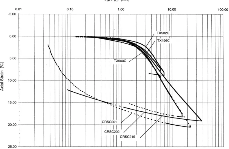
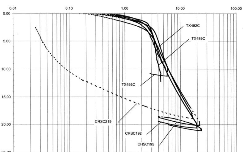
Figure 3.18 Summary of compression curve obtained from CRSC tests 104 (data from Varney, 1998) and triaxial tests (data from this

research) of layer C.

Figure 3.19 Summary of compression curve obtained from CRSC tests 105 (data from Varney, 1998) and triaxial tests (data from this

research) of layer D.

Figure 3.20 Summary of compression curve obtained from CRSC tests 106 (data from Varney, 1998) and triaxial tests (data from this

- research) of layer E.

Figure 3.21 Recompression and Compression ratio of 1-95 site. 107

(20)

-Figure 3.22 Summary of the normalized undrained shearing behaviors 108 of the natural BBC obtained from the CKoUC (NC) tests.

Figure 3.23 Summary of the normalized undrained shearing behaviors 109 of the natural BBC obtained from the CKoUC (OCRs of 2) tests.

Figure 3.24 Summary of the normalized undrained shearing behaviors of 110 the natural BBC obtained from the CKQUE (NC) tests

Figure 3.25 Indication of critical state shear stress. 11

Figure 3.26 SHANSEP plot 112

Figure 3.27 Capability of small strain measurement device compared to 113 the conventional LVDTs based external strain measurements.

Figure 3.28 Summary of the normalized undrained modulus of the natural 114 BBC obtained from the CKOUC (NC) tests.

Figure 3.29 Summary of the normalized undrained modulus of the natural 115 BBC obtained from the CKoUC (OCRs of 2) tests.

Figure 3.30 Summary of the normalized undrained modulus of the natural 116 BBC obtained from the CKOUE (NC) tests

Figure 4.1 Example of input file e3_09. 135

Figure 4.2 Example of input file e3_28. 135

Figure 4.3 Definition of Load Reversal Point for the swelling and 137 reloading case.

Figure 4.4 Reference frame used for the strain input of the element 138 simulation program.

Figure 4.5 Example of output file monoTC.res and a compression 139 curve generated from the file.

Figure 4.6 Example of output file bounding.res with an example plot 140 of bounding surface generated from the output file.

Figure 4.7 Example of the output file ccdraw.res with a compression 141 curve plotted based on the data in ccdraw.res.

Figure 4.8 Example of the output file uudraw.res with a normalized 142 undrained shearing curve generated from the file.

(21)

-Figure 4.9 Usual steps of simulations used to obtain a comparable shearing 143 prediction to the laboratory test results.

Figure 4.10 One of the conventional steps of simulation used to obtain 143 a comparable consolidation prediction to the laboratory

test results.

Figure 4.11 Strain histories at the centerline of tube samples 144 (After Baligh et al., 1987).

Figure 4.12 Diagram shows the proposed steps of simulation used in 145 this research

Figure 4.13 Yield surface used in MIT-E3 soil model for normally 146 consolidated clays(After Whittle, 1987).

Figure 4.14 Example of output from Yield Surface drawing subroutine 147 Figure 5.1 Graphical illustration of Elasto-Plasticity definition. 177 Figure 5.2 Yield surface used in MIT-E3 soil model for normally 178

consolidated clays.

Figure 5.3 Schematic drawing illustrated the Stress Reversal Point (SRP) 179 and the state of stress defined by the distance from the SRP

and loading direction

Figure 5.4 Definition of 4 for hydrostatic conditions. 180

Figure 5.5 Steps used in the new proposed simulations including the 181 Sample Disturbance Simulation (SDS) processes.

Figure 5.6 Effects of eo parameter on the consolidation behavior. 182 Figure 5.7 Effects of eo on the undrained shearing behavior. 182 Figure 5.8 Effects of A parameter on the consolidation behavior. 183 Figure 5.9 Effects of A parameter on the undrained shearing behavior. 183 Figure 5.10 Effects of C parameter on the consolidation behavior. 184 Figure 5.11 Effects of C parameter on the undrained shearing 184

behavior.

Figure 5.12 Effects of n parameter on the consolidation behavior. 185 Figure 5.13 Effects of n parameter on the undrained shearing 185

behavior.

(22)

-Figure 5.14 Figure 5.15 Figure 5.16 Figure 5.17 Figure 5.18 Figure 5.19 Figure 5.20 Figure 5.21 Figure 5.22 Figure 5.23 Figure 5.24 Figure 5.25 Figure 5.26 Figure Figure Figure Figure Figure 5.27 5.28 5.29 5.30 5.31

Effects of h parameter on the predicted consolidation behavior.

Effects of h parameter on the predicted undrained shearing behavior.

Comparison of the variation of Ko(oc) versus OCR obtained from MIT-E3 and that obtained from the empirical equation

(5.42) and the test data (After Ganendra and Potts, 1995).

Effects of 2G/K parameter on the predicted consolidation behavior. Effects of 2G/K parameter on the predicted undrained shearing

behavior.

Effects of changing $'Tc on the predicted compression undrained shearing behavior.

Effects of changing O'TE on the predicted extension undrained shearing behavior.

Effects of c parameter on the predicted consolidation behavior. Effects from c parameter on the predicted undrained shearing

behavior.

Effects from S, parameter on the predicted undrained shearing behavior.

Minor effects from S, parameter on the predicted consolidation behavior.

Effects of c> parameter on the predicted normalized undrained modulus.

Effects of yparameter on the predicted undrained shearing behavior.

Minor effect of yparameter on the predicted compression curve. Effects of 1o parameter on the predicted consolidation behavior.

Effects of ico parameter on the predicted undrained shearing behavior.

Schematic drawing illustrated the definition of Ko.

Effects of Wo on the predicted compression curve.

- 22 -186 186 187 187 188 188 189 189 190 191 192 192 193 193 194 194 195 196

(23)

Figure 5.32 Figure 5.33 Figure 5.34 Figure 5.35 Figure 5.36 Figure 5.37 Figure 5.38 Figure 5.39 Figure 5.40 Figure 5.41 Figure 5.42 Figure 5.43 Figure 5.44 Figure 5.45 Figure 5.46

Effects of yo on the predicted normalized undrained shearing curve.

Predicted compression curve based on the parameter obtained from the triaxial tests and those proposed by Whittle, 1993. Evolutions of yield surface during the simulation processes. Variation of the predicted compression curve with varying Vo parameter as compared to the triaxial test results.

The variation of the predicted octahedral stress at the end of 1-dimensional consolidation with varying y1o parameter as

compared to the octahedral stress obtained from the corresponding triaxial tests.

Comparison of the predicted compression curve based on the original parameters with that of TX485 test.

Comparison of the predicted compression curve based on the Best Fit parameters with that of TX485 test.

Comparison of the predicted compression curve based on the Best Fit parameters with that of TX486 test.

-23 -196 197 197 198 198 199 199 200 200 201 201 202 202 203 203

(24)

Figure 5.47 Figure 5.48 Figure 5.49 Figure 5.50 Figure 5.51 Figure 5.52 Figure 5.53 Figure 5.54 Figure 5.55 Figure 5.56 Figure 5.57 Figure 5.58 Figure 5.59 Figure 5.60

Comparison of the predicted compression curve based on the Best Fit parameters with that of TX495 test

Comparison of the predicted normalized undrained compression (NC) shearing behavior based on the original parameters, with

that of TX485 test.

Comparison of the predicted undrained compression shearing based on Best Fit parameters with that of TX485 test.

that of TX489 test.

Comparison of the predicted undrained compression shearing based on Best Fit parameters with that of TX489 test.

that of TX500 test.

Comparison of the predicted undrained compression shearing based on Best Fit parameters with that of TX500 test

- 24 -204 204 205 205 206 206 207 207 208 208 209 209 210 210

(25)

Figure 5.61 Figure 5.62 Figure 5.63 Figure 5.64 Figure 5.65 Figure 5.66 Figure 5.67 Figure 5.68 Figure 5.69 Figure 5.70

Comparison of the predicted normalized undrained extension shearing (NC) based on the original parameters with that of TX486 test.

Comparison of the predicted undrained extension shearing behavior based on the Best Fit parameters with TX486 test results.

Comparison of the predicted undrained compression shearing (OCRs of 2) based on the original parameters with that of TX488 test.

Comparison of the predicted undrained compression shearing (OCRs of 2) based on the Best Fit parameters with TX488 test results.

Comparison of the predicted undrained compression shearing (OCRs of 2) based on the original parameters with that of TX495 test.

Comparison of the predicted undrained compression shearing (OCRs of 2) based on the Best Fit parameters with TX495 test results.

- 25 -211 211 212 212 213 213 214 214 215 215

(26)

Figure 5.71 Comparison of the predicted undrained compression 216 shearing (OCRs of 2) based on the original parameters

with that of TX502 test.

Figure 5.72 Comparison of the predicted undrained compression 216 shearing (OCRs of 2) based on the Best Fit parameters

with TX502 test results

Figure 6.1 Strain history due to tube sampling processes 230 (After Baligh et al., 1987).

Figure 6.2 Flowchart shows the general framework for soil model 231 input parameter selection procedures.

Figure 6.3 Flowchart shows framework for MIT-E3 input parameter 232 selection procedures.

Figure 6.4 Comparison of the predicted compression curve based on 233 the Best Fit input parameters with that of TX485 test.

Figure 6.5 Comparison of the predicted normalized undrained shearing 233 curve based on the Best Fit input parameters with that of

TX485 test.

Figure 6.6 Comparison of the predicted compression curve based on 234 the Best Fit input parameters with that of TX489 test.

Figure 6.7 Comparison of the predicted normalized undrained shearing 234 curve based on the Best Fit input parameters with that of

TX489 test.

Figure 6.8 Comparison of the predicted compression curve based on 235 the Best Fit input parameters with that of TX500 test.

Figure 6.9 Comparison of the predicted normalized undrained shearing 235 curve based on the Best Fit input parameters with that of

TX500 test.

Figure 6.10 Comparison of the predicted compression curve based on 236 the Best Fit input parameters with that of TX486 test.

(27)

-Figure 6.11 Figure 6.12 Figure 6.13 Figure 6.14 Figure 6.15 Figure 6.16 Figure 6.17 Figure 6.18 Figure 6.19 Figure 6.20 Figure 6.21

Comparison of the predicted normalized undrained shearing curve based on the Best Fit input parameters with that of TX486 test.

Comparison of the predicted compression curve based on the Best Fit input parameters with that of TX492 test.

Comparison of the predicted compression curve based on the Best Fit input parameters with that of TX495 test. Comparison of the predicted normalized undrained shearing

curve based on the Best Fit input parameters with that of TX495 test.

Comparison of the predicted compression curve based on the Best Fit input parameters with that of TX502 test. Comparison of the predicted normalized undrained shearing

curve based on the Best Fit input parameters with that of TX502 test. - 27 -236 237 237 238 238 239 239 240 240 241 241

(28)

(29)

-28-List of Symbols

b Orientation tensor for bounding surface

S Deviatoric stress tensor

P Direction of plastic flow at first yield for OC clays

P Direction of plastic strain increments (flow direction tensor)

BBC Boston Blue Clay

C Material constant controls the non-linearity in the volumetric response c Ratio of major/minor semi-axes of bounding surface ellipse

CKoUC/E Ko-consolidated undrained shear test, compression/extension

CR Virgin compression ratio

CRSC Constant rate of strain consolidation

C, Coefficient of Consolidation

DSS Direct simple shear test

e Void Ratio

eo Void ratio at the reference stress, a'OCT = 1 unit

Eu Undrained Modulus

Eu(max) Maximum Undrained Modulus

G Elastic Shear Modulus

Gmax Maximum elastic shear modulus at small strain level

H Elasto-plastic modulus

K Elastic Bulk Modulus

Ko Coefficient of lateral earth pressure at rest LVDT Linear voltage displacement transducer

h Material constant for bounding surface plasticity

n Material constant controls the non-linearity in the volumetric response

NC Normally consolidated

OC Overconsolidated

OCR Overconsolidation Ratio

(30)

-OCR, OED PI PL RBBC rc rx sec SHANSEP SR SSM St tan TX VCL a a0 Ea Evol $'TC O'TE Y KO A V v H - 30 -Overconsolidated ratio at K0 of 1 Oedometer test Plasticity Index Plasticity Limit

Resedimented Boston Blue Clay Scalar distance mapping for flow rule

Scalar distance mapping for hardening rule for bounding surface rotation Secant

Stress History And Normalized Soil Engineering Properties Swelling ratio

Small Strain Measurement Device

Material constant controls the post-peak undrained shearing behavior tangent

the undrained shearing Triaxial test

Virgin compression line Natural water content

Size of bounding surface

Size of load surface for OC clay Size of load surface at first yield Axial strain

Volumetric strain

Friction angle at large strain, triaxial compression test Friction angle at large strain, triaxial extension test

Material constant for bounding surface mapping of flow direction Compressibility parameters at load reversal

Slope of the Virgin Compression Line in the e-loga'OCT space Poisson's ratio

Octahedral effective stress Horizontal effective stress

(31)

G'ocT Octahedral effective stress

G' PPreconsolidation pressure G v Vertical effective stress

o Material constant controls the behavior at the small strain level during 4, s Scalar distance parameters used in perfectly hysteretic model

yo Material constant controls rate of yield surface evolution and changes in its size

(32)

(33)

Chapter 1 Introduction

1.1 Problem Statement

One of the most challenging problems for the geotechnical profession is the prediction of ground movement. Incorporated with complex soil behavior and usually very small allowance in the predictions, the task becomes very difficult. The problem is much more difficult when dealing with a large-scale project in the urban area where the ground deformation is the most concerning issue. There are numerous efforts in the development of advanced laboratory testing techniques (i.e., Sheahan, 1991, Santagata, 1998) and soil models (i.e., Kavvadas, 1982, Whittle, 1987, Pestana, 1994) to help describe and enhance the prediction capability of the geotechnical profession.

Nevertheless, precise predictions can only be achieved when careful investigation of soil behavior and appropriate uses of soil models including an appropriate selection of model input parameters are employed. The calibration or the method of selecting a set of representative input parameters for the soil model used in the engineering projects has now become a very important issue. The input parameters, essentially, control the predicted results and therefore the appropriate set of input parameters is required in order to obtain reliable predictions for use in the engineering projects.

For a complicated and advanced soil model, the input parameters are separated into two categories: 1) direct input parameters and 2) Indirect input parameters. The direct input parameters can be directly obtained from the interpretation of a set of reliable laboratory tests while the indirect input parameters can only be obtained via a parametric study using the element simulation program. While the input parameters play an important role in the prediction of ground movement, there is no established rational framework for soil model input parameter selection procedures.

The existing method of selection of input parameter is ambiguous especially for the consolidation behavior simulations of natural soils. The initial state of stress is subjectively

(34)

-selected and no sampling disturbance effect is assessed in the existing method. Based on the existing method, the input parameters are obtained from appropriate laboratory tests (for those can be obtained directly) and from suitable parametric studies based on the conventional simulation procedure (for those cannot be obtained directly from the laboratory tests). The conventional simulation assumes no Sampling Disturbance effects in the simulation process. The simulation is, generally, start with the element consolidation

along the Virgin Compression Line (VCL) and then follows K-unloading to the selected octahedral effective stress prior performs the consolidation simulation. The starting point of the consolidation simulation (after K-unloading) is subjectively selected and limited by the capability of the selected model to predict the overconsolidated behavior of soils.

1.2 Research Objectives

The overall objective of this research is to develop a rational framework of soil model input parameter selection to account for the Sampling Disturbance effects. The Sampling Disturbance processes are incorporated into the element simulation program to simulate the strain (or stress) history that the soil specimen experienced prior to laboratory testing. The Strain Path Method (SPM) (Baligh, 1985) is utilized to predict the strain history due the standard Shelby Tube sampling processes. The complete strain history used in this research combines the ideal tube sample processes with the hydrostatic swelling after shear stress release process to account for more realistic soil behaviors.

The MIT-E3 effective stress soil model (Whittle, 1987) is used throughout the research in the element simulation program. The model is selected based on its capability in modeling the complex soil behavior including changes in anisotropic directions and behaviors in the lightly to moderately overconsolidated range (OCRs of 2 to 4).

This research program is also designed to extend the database of natural Boston Blue Clay properties and the understanding of its behaviors. The natural Boston Blue clay samples used in this research were obtained from 1-95 site, Saugus, Massachusetts (Varney, 1998). The site has been the MIT testing site since the mid-1960's. Series of triaxial tests are performed in this research to investigate the stress-strain-strength behavior of the natural Boston Blue Clay. Totally, nine best quality tests are selected to use in this research as a reference for the MIT-E3 soil model. All specimens used in the triaxial tests

(35)

-performed in this research are equipped with the Small Strain Measurement devices (Santagata, 1998) to investigate the soil behavior at the small strain region.

1.3 Thesis Organization

The research began with the investigation of natural Boston Blue Clay behavior through a series of triaxial tests following the SHANSEP1 technique, which is-used as a standard of testing at MIT Geotechnical Laboratory. All samples were obtained from 1-95 site, Saugus, Massachusetts because the soil data and behavior of natural BBC at this site are well defined and studied. Background of the research is presented in Chapter 2 including the fundamental properties of natural BBC and soil profile, brief background of MIT-E3 soil model, and the basic theory of sampling disturbances and their effects on the compressibility and shearing behavior of soils.

Chapter 3 presents details of triaxial test procedures and results of the test program. A series of triaxial tests were performed and nine of the best quality tests are selected for the simulations. Two methods of quality assessment are used in this research. Terzaghi et al., 1996 proposes the first method investigating the strain at the insitu vertical effective stress versus the elevation. While the method is simple and can be adapted easily, it can yield misleading evaluation of the sample disturbance especially for the nearly normally consolidated soils (OCRs of 1.0 to 1.5) at depth. A proposed assessment technique is presented which bases the quality of specimens on the variation of strain at in situ vertical effective stress with OCR. Detail discussions on both techniques are provided in the Chapter 3.

All test specimens are equipped with the Small Strain Measurement devices (SSM) to investigate the soil behaviors at the small strain region (Ea of 0.0001% an higher) and the results are used in the development of the framework for MIT-E3 soil model. Three samples from each layer are used for the analyses. Two samples were tested in the mode of Ko-Consolidation Undrained Triaxial Compression and Ko-Consolidation Undrained Extension test on normally consolidated sample. The third specimen was tested in

Ko-SHANSEP is "Stress History And Normalized Soil Engineering Properties" (Ladd and Foott, 1974).

(36)

-Consolidation Undrained Compression on overconsolidated sample (OCR's of 2). The soil profile used in this research was adopted from Morrison, 1984.

Chapter 4 provides details of developments to the element simulation program. The element simulation program was developed at MIT for use in the evaluation of soil models and for the parametric study to obtain a set of representative input parameters. The theoretical basis of the sampling disturbance are provided in this chapter including the concept of ideal tube sampling processes (Baligh, 1985), actual tube sampling processes (Ladd and Lambe, 1963), and the proposed complete steps used in this research for all simulations. The new subroutine for Sample Disturbance Simulation is discussed with other important modifications of the computer program.

Chapter 5 presents the formulation of MIT-E3 soil model and the simulation results. Extensive discussions on the effects of each input parameter used in MIT-E3 soil model on the predicted consolidation and undrained shearing behaviors are provided in the Chapter. The simulation results serve as references for the development of framework for soil model input parameter selection procedures.

Chapter 6 presents the generalized framework for soil model input parameter selection procedures. The specific framework for MIT-E3 soil model is also provided in this chapter based on the extensive simulation results performed by the new proposed element simulation processes.

Discussion and conclusion of this research are provided in Chapter 7 with recommendations for further research to gain better understanding of natural clay behavior and framework for soil model input parameter selection procedures.

1.4 References

1. Baligh M.M. (1985), Strain Path Method, Journal of geotechnical Engineering, ASCE 111, No.9, pp. 1108-1135.

2. Juan Manuel Pestana-Nascimento (1994), A Unified Constitutive Model for Clays and

Sands, Massachusetts Institute of Technology, PhD Thesis.

3. Ladd C.C. (1991), Stability Evaluation During Staged Construction, Journal of Geotechnical Engineering, 117(4), pp. 537-615.

(37)

-4. Ladd C.C., Whittle A.J., Legaspi D.E. (1994), Stress-Deformation Behavior of an Embankment on Boston Blue Clay, Proceedings of Settlement' 94, Geotechnical Engineering Division/ASCE, pp. 1730-1759

5. Morrison M.J. (1984), In Situ Measurements on A Model Pile in Clay, Massachusetts Institute of Technology, PhD. Thesis.

6. Santagata M.C. (1994), Simulation of Sampling Disturbance in Soft Clays Using Triaxial Element Tests, Massachusetts Institute of Technology, SM. Thesis.

7. Santagata M.C. (1998), Factors Affecting the Initial Stiffness and Stiffness Degradation of Cohesive Soils, Massachusetts Institute of Technology, PhD. Thesis. 8. Sheahan T.C. (1991), An Experimental Study of Time-Dependent Undrained Shear

Behavior of Resedimented Clay Using Automated Stress-Path Triaxial Equipment,

Massachusetts Institute of Technology, ScD. Thesis.

9. Sheahan T.C., Germaine J.T., Ladd C.C. (1990), Automated Triaxial Testing of Soft Clays: An Upgraded Commercial System, Geotechnical Testing Journal, GTJODJ,

13(2), pp. 153-163.

10. Terzaghi K., Peck R.B., Mesri G. (1996) Soil Mechanics in Engineering Practice, John Wiley & Sons, New York, 549 pp.

11. Varney A.J. (1998), A Performance Comparison between A Novel Tapered Piezoprobe and The Piezocone in Boston Blue Clay, Massachusetts Institute of Technology, SM. Thesis.

12. Whittle A.J. (1987) A Constitutive Model for Overconsolidated Clays with Application to The Cyclic Loading of Friction Piles, Massachusetts Institute of Technology, PhD. Thesis.

13. Whittle A.J. (1993), Evaluation of a constitutive model for overconsolidated clays, Geotechniques 43, No.2, 289-313.

14. Whittle A.J., DeGroot D.J., Ladd C.C., Seah T.H. (1994), Model Prediction of Anisotropic Behavior of Boston Blue Clay, Journal of Geotechnical Engineering, 120(1), 199-224

(38)

(39)

-38-Chapter 2

Background

This chapter presents the background of the 1-95 site where there has been a MIT Geotechnical testing site for the past four decades. The samples for this laboratory test program are obtained from the site in 1997 (Varney et al., 1997). Extensive tests have been performed to improve understanding of soil behavior and as a part of database collections

for research purposes.

2.1 Background of 1-95 Site

The 1-95 site has been the MIT testing site since the mid-1960's. The site is approximately 10 miles North of MIT, located in the Rumney Marsh at the southern town line in Saugus, Massachusetts. The MIT Geotechnical group originally became involved with the site during the design phase for extending Interstate highway, 1-95, through the Metropolitan Boston. Instrumentation programs were conducted at Station 246 and 263 from 1967-1969 to monitor the deformation during the construction process. A Field Vane and laboratory testing programs were conducted by MIT and the soil properties were used in a prediction symposium, which held at MIT in 1974. The symposium included full scale loading to failure of the Station 263 where the fill was obtained from Station 246. Profession predictions of the embankment failure from many well-known geotechnical research groups served as a benchmark for the state of the profession.

Over the past 20 years, MIT has returned to the test site to evaluate new devices and collect soil samples. To prepare the site for field investigation and soil sampling, a 18 to 24 inch thick sand mat was placed over the marsh peat deposits to the East of the embankment at Station 246 and to the West of the embankment at Station 263. The sand mats served as working platforms for a number of field investigations over the past 20 years. The sand mat at Station 246 was extended to the North, increasing the area available for field testing in the early of 1980s.

(40)

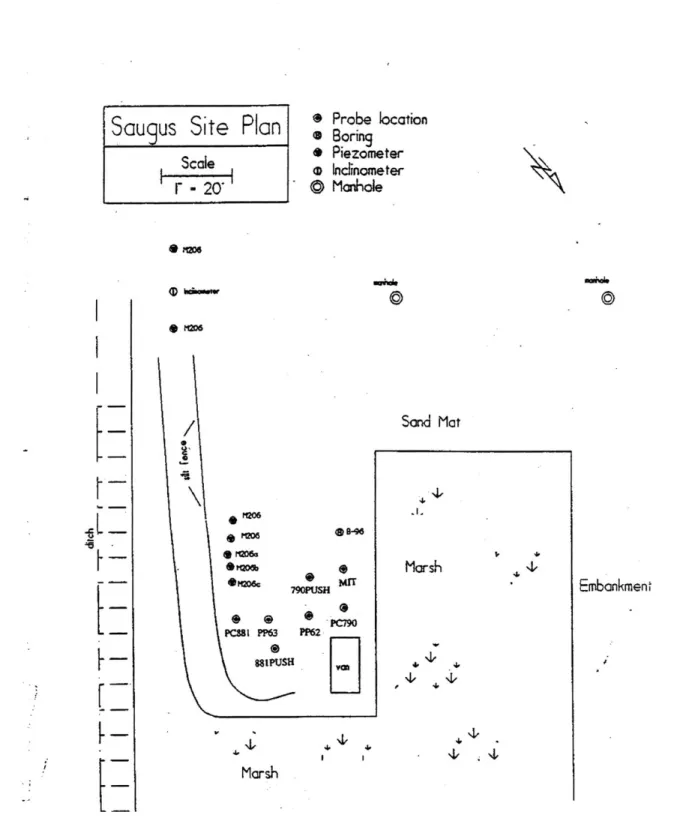
-A detailed plan of the northern extension of the Station 246 site is presented in Figure 2.1 including the locations of the boreholes for soil sampling. The plan also

includes the two manholes, which connect to the original instrumentation tunnel. These manholes serve as the reference makers for the site. The soil sampling program was conducted on the northern end of the extended mat at the Station 246. The undisturbed samples were obtained from Boring B-96 and used in this research for three series of triaxial tests (Varney et al., 1997). All elevations referred to in this research are referenced to the 1929 NGVD (National Geodetic Vertical Datum) datum.

2.2 Soil Profile and Summary of Soil Properties of The Natural

Boston Blue Clay

This section provides the summary of the soil properties and soil profile used in this research. The first three sections describe the BBC properties categorized into 1) fundamental properties including water content profile (uncorrected and corrected), salt concentration profile and total unit weight profile, 2) preconsolidation pressure and 3) compressibility and normally consolidated coefficient of consolidation. The sections summarize the soil properties based on both the prior data (Ladd et al, 1994) and the relatively new data (from Varney, 1998 and this research). The last section provides the brief descriptions of the soil profile selected as the reference for this research.

2.2.1 Fundamental Properties of The Natural Boston Blue Clay

The fundamental properties of natural BBC at 1-95 site including Atterberg limit and salt concentration are performed on samples from every tube (Varney, 1998). The Boston Blue Clay can be categorized as a low plasticity clay (CL as shown in Figure 2.2) based on the Unified Soil Classification System (USCS). The plasticity index varies between 15 to 30% and is lower and more variable in the upper 50 ft.

Figure 2.3 presents the water content profile at the site with the Plastic and Liquid Limit. Due to the salt concentration in the water, the water contents must be corrected since the salt in the pore fluid affects the engineering and index properties of the clays. Figure 2.4 shows the salt concentration profile at the site. Salt concentration of the clays is

(41)

-highest at the upper crust and decrease with decreasing elevation. The corrected water content can be obtained based on the salt concentration and measured water content, by ASTM D2216-92, based on equation (2.1).

w' = .(2.1)

1C -+W

Where w' is the corrected water content [%]

w is the measured water content from the specimens [%] C is the salt concentration in the specimen [gil]

yc is the unit weight of salt [g/cc]

The Plastic and Liquid Limit are also affected from the salt concentration and can also be corrected by the equation (2.1). Figure 2.5 presents the corrected water content from salt concentration with Atterberg limit plotted versus elevation. The water contents are increasing with depth starting from approximately 38% at the -5m elevation and increasing gradually reaching nearly constant values of 50% at -15 m elevation.

Figure 2.6 presents the summary of the total unit weight of the natural BBC at the site (Varney, 1998). The total unit weight of the BBC is in the range of 1.77 to 1.85 g/cc vary with elevation. The proposed line used in the in situ stress calculation is also presented in the Figure.

2.2.2 Preconsolidation Pressure

Natural Boston Blue Clay at the 1-95 site has been very well studied over the past 30 years. Extensive summary of soil properties at this site was presented by Ladd et al. (1994). The preconsolidation profile from Ladd et al. is presented in Figure 2.7a. The profile was obtained from the prior data at the site before 1994.

As shown in Figure 2.7a, some of preconsolidation pressures obtained from the 1966 and 1980 oedometer tests lie below the vertical effective stress line, which indicates the high degree of disturbance of the samples. The resulting preconsolidation pressures are

(42)

-41-also highly scattered both in the overconsolidated and nearly normally consolidated range, above and below approximately -22 m elevation, respectively.

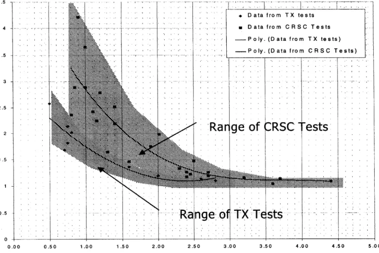
The most recent testing program at MIT, using automated controlled testing system, yielded a valuable set of data obtained from Constant Rate of Strain tests (CRSC tests). The data from the tests were collected by Data Acquisition System (DAQ), which resulted in the continuous data collection giving better defined and more reliable results as compared to the discrete data collection in the past. The preconsolidation profile was better defined. Figure 2.7b shows the preconsolidation pressure profile obtained from the CRSC and TX tests. The CRSC test results are used to compare with the triaxial testing results obtained from this research. While CRSC tests yield valuable data of consolidation behavior, the triaxial tests give both consolidation and stress-strain-strength behavior. Complete soil behaviors of 1-95 site can be achieved upon combining all test results and consider the prior data. Figure 2.8 presents the summary of OCR profile based on the data from CRSC tests (data from Varney, 1998) and triaxial tests (data from this research).

2.2.3 Compressibility and Coefficient of Consolidation

Figure 2.9 presents the summary of the compressibility of the BBC in terms of maximum compression ratio (CRmax). Figure 2.9a shows the profile of CRmax based on data from Ladd et al, 1994 and other prior data. The CRmax profile indicates that the compressibility gradually increases with depth. Figure 2.9b presents the profiles of Recompression Ratio at the in situ vertical effective stress (RR) and CRmax obtained from the CRSC tests (data from Varney, 1998) and triaxial tests (data from this research). The trend of the CRmax profile is similar to that of Figure 2.9a except at the elevation below elevation -22.00 m where the new data indicates lower and fairly constant with depth values of CRmax. It should be noted that there are two points in Figure 2.9b, which CRmax

are much differ from the general trend (noted as point A and B in the Figure). The deviations may be caused by the local variability of the natural BBC.

Figure 2.10 presents the normally consolidated coefficient of consolidation (Cv(NC)) based on data from Ladd et al. and other prior data. Figure 2.10(a) shows the Cv(NC) profile based on the data from Ladd et al. The Cv(NC) are quite scattered in the

(43)

-upper crust (at elevation higher than -12.00 m) while they are more consistent below the elevation -12.00 m.

Figure 2.10(b) presents the more recent C(NC) profile based on the data obtained from Varney, 1998. The CV(NC) presented in the Figure are selected based on the vertical effective stress of 10 ksc. In overall, the C(NC) profile is less scatter in the elevation lower than -12.00 m. The trend is, essentially, the same except that the Cv(NC) values are a little bit higher than those presented by Ladd et al. This may be caused by the-difference in the selecting of the reference vertical effective stress.

2.2.4 Soil Profile

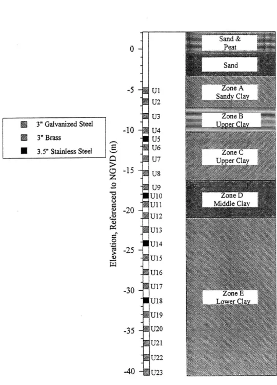
The soil profile used in this research is based on Morrison, 1984. The soil profile was selected for use in triaxial and previous CRSC tests. The profile is based on a number of the field and sampling programs performed by Morrison as the part of the study of shaft capacity of axial loaded piles driven in clay. Figure 2.11 presents the soil profile with the location of undisturbed samples (Varney et al., 1997) for this laboratory test program. The samples used in the triaxial testing program in this research are obtained from the layer C, D and E, based on the Morrison proposed soil profile. The selected layer covers a range of OCR ranging from approximately 1.1 to 3.0 where the coefficients of consolidation, C., are quite consistent.

2.3 MIT-E3 Soil Model

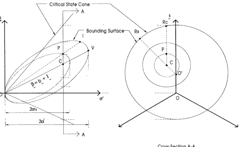
The MIT-E3 soil model is an effective stress soil model, which can describe behavior of normally to moderately overconsolidated clays (OCRs up to 4). The model is formulated based on three key elements namely 1) elasto-plasticity, 2) Hysteretic model, and 3) Bounding Surface model. Consideration of some of the key model formulations is discussed in Chapter 4. Figure 2.12 shows yield surface for normally consolidated clays used in MIT-E3 effective stress soil model.

The model was developed at MIT to predict the behavior of clays (normally to moderately overconsolidated) under cyclic loading conditions (Whittle, 1987). The model has been investigated and evaluated comprehensively for its representation of shearing

(44)

-behavior (DeGroot, 1989 and Whittle, 1990b, Seah, 1990). However, little information exists regarding the accuracy of the predicted consolidation behavior. Therefore, the simulations performed in this research focus on consolidation behavior and will serve as a database for evaluations of the model on the predictive capability of consolidation behavior of natural BBC.

2.4 Sampling Disturbance

Table 2.1 summarizes the sources of disturbance, which can occur during sampling of cohesive soils from a drill hole. The sampling disturbance changes the soil so that the laboratory measured properties are different from the in situ properties. Sampling Disturbance causes a reduction in the peak undrained strength, an increase in the drained compressibility during recompression, and a decrease in the virgin compression ratio. These effects can lead to serious misinterpretation of field behavior. Figure 2.13 shows the schematic drawing illustrating the effects from sampling disturbance on the undrained shearing behavior while Figure 2.14 presents its effects on the drained compressibility.

The development of special sampling techniques (i.e., the Sherbrooke 250 mm diameter block sampler, Lefebvre and Poulin (1979), and the Laval 200 mm diameter overcored tube sampler, La Rochelle et al. (1981)), to obtain extremely high quality samples shows significant differences in drained compressibility and peak triaxial strength (drained and undrained) as compared to those from conventional fixed piston samples, Jamiolkowski et al. (1995). However, these large diameter samplers are either too expensive for most geotechnical investigations or are not feasible for very deep sampling and for offshore exploration. Moreover, other sources like those associated with stress relief, and especially the outgassing problem often encountered in deep water deposits, are impossible to minimize without taking extreme measures.

Given the above constraints, most sampling programs must employ procedures that may yield samples of less than ideal quality. Hence, practicing engineers need techniques for assessing the sample quality and knowledge of testing techniques that might be employ to minimize the adverse effects of sample disturbance, Jamiolkowski et al. (1995).

(45)

-Numerous efforts have been employed to study the effects of sampling disturbance both theoretically (Baligh et al., 1987) and practically (Santagata, 1994). Ladd and Lambe, 1963, proposed a hypothetical stress path to emphasize the importance of the sampling disturbance effects on the laboratory test results. Baligh et al., 1987, theoretically, explained the sampling disturbance procedures of variety shapes and configurations of the tube samplers based on the Strain Path Method (SPM). Detailed discussion on the Ideal Tube Sampling process (based on SPM by Baligh, 1985) and the Actual Tube Sampling process (Ladd and Lambe, 1963) are provided in Sections 2.4.1 and 2.4.2, respectively.

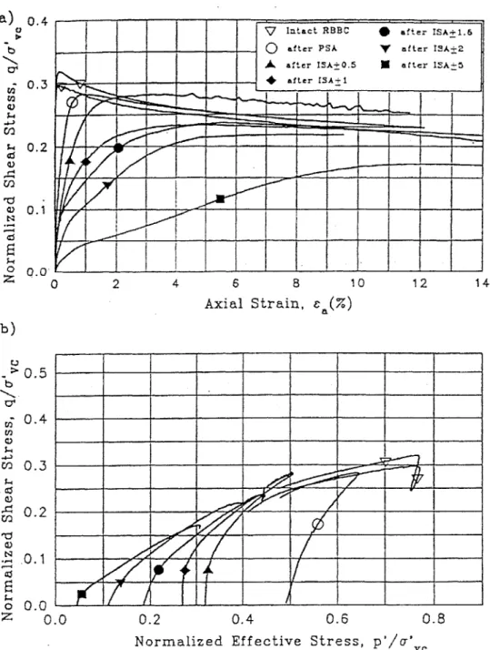
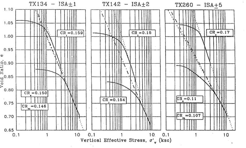
The utilization of the SPM opened a new way to investigate the sampling disturbance effects by incorporating the SPM strain predictions with the advanced soil model (i.e., MIT-E3 and MIT-S1). Santagata (1994) performed a series of laboratory tests on the Resedimented Boston Blue Clay (RBBC) simulating the stress history experienced by the soil samples during the sampling process and investigated the subsequent effects on the resulting consolidation and shearing behaviors. The test results emphasize the effects of sampling disturbances on the drained compressibility and undrained shearing. As shown in Figure 3.15, tremendous changes in undrained shearing behavior occur when the specimens are subjected to cycles of undrained shearing to various degree of disturbance (the similar processes to what the soil specimen experienced during the sampling processes). Figure 3.16 shows the effects of disturbances on the soil compressibility. It should be noted that Figure 3.16 presents data from ISA tests, which refer to Ideal Sampling Approach with varying amounts of strain cycles (denoted by number after ISA).

The following sections present the detailed discussion on the Ideal Tube Sampling process (Baligh et al., 1987) and Actual Tube Sampling Process (Ladd and Lambe, 1963). These two approaches provide the basic framework of the proposed Sampling Disturbance Simulation (SDS) process used in this research. The details of the proposed steps used in the SDS are provided in Chapter 4.