Design and control of a Two-Degree-of-Freedom powered ankle-foot prosthesis

Design and Control of a Two-Degree-of-Freedom

Powered Ankle-Foot Prosthesis

by

Tsung-Han Hsieh

B.Sc., National Taiwan University (2013)

LIBRARIES

M.Sc., Carnegie Mellon University (2015)

ARCHIVES

Submitted to the Program in Media Arts and Sciences,

School of Architecture and Planning

in partial fulfillment of the requirements for the degree of

Master of Science in Media Arts and Sciences

at the

MASSACHUSETTS INSTITUTE OF TECHNOLOGY

September 2019

©Massachusetts

Institute of Technology 2019. All rights reserved.

Signature redacted

A uthor ...

...

Program in Media Arts and Sciences,

SIAugust

8, 2019

Signature redacted

C ertified by ...

...

Hugh Herr

Professor of Media Arts and Sciences

Thesis Supervisor

Signature

redacted-A ccepted by

...

I

...

/

/

Tod Machover

Design and Control of a Two-Degree-of-Freedom Powered

Ankle-Foot Prosthesis

by

Tsung-Han Hsieh

Submitted to the Program in Media Arts and Sciences,, School of Architecture and Planning

on August 8, 2019, in partial fulfillment of the requirements for the degree of

Master of Science in Media Arts and Sciences

Abstract

Powered ankle prostheses have been proven to improve the walking economy of transtibial amputees although these powered systems are usually much heavier in weight than conventional prostheses. All commercial powered ankle prostheses that are currently available can only perform one-degree-of-freedom motion in a limited range. However, the human ankle can perform both frontal and sagittal plane mo-tions. Studies have shown that the frontal plane motion during ambulation is associ-ated with balancing. As more advanced neural interfaces have become available for amputees, it is possible to fully recover ankle function by combining neural signals and a robotic ankle. Accordingly, there is a need for a powered ankle prosthesis that can have active control on not only plantarflexion and dorsiflexion but also eversion and inversion.

The objective of this thesis is to design and evaluate a two-degree-of-freedom powered ankle-foot prosthesis that is untethered and can support an average size human for level-ground walking with full power. At present, a system with such capabilities only exists as tethered.

The prosthesis presented in this thesis is a second-iteration design based on its predecessor. The new design features a larger joint range of motion, a more robust transmission, and a more powerful battery module. Benchtop tests and walking trials were conducted to evaluate the system. The results demonstrate system characteris-tics and dynamics and the ability to support body weight in level-ground walking.

Thesis Supervisor: Hugh Herr

I

Design and Control of a Two-Degree-of-Freedom Powered

Ankle-Foot Prosthesis

by

Tsung-Han Hsieh

The following people served as readers for this thesis:

Signature redacted___

T hesis R eader ...

...

Edward Boyden

Professor of Media Arts and Sciences

Y. Eva Tan Professor in Neurotechnology

Massachusetts Institute of Technology

Signature redacted

Thesis Reader ...

.

..

/I~rtmut

Geyer

Associate P/fessor of Robotics

Carnegie Mellon University

Acknowledgments

I'd like to thank my advisor, Hugh Herr, for all the resource and support he gave me. Also a huge thank to my thesis readers, Ed Boyden and Hartmut Geyer, for supporting me through my academic endeavors.

Thanks Matt Carney, for teaching me how to do mechanical design like a pro. Thanks Seong Ho Yeon and Tony Shu, for working together during these days. Thanks Emily Rogers for helping me use the water jet machine. Thanks Mark Belanger, the best shop manager in the world. Thank you for being so patient with me and helping me with all the machining work. I love you. You are the best.

Thanks Mayday, my favorite band when I was in high school (and only in high school). I listened to your songs everyday for the past two week and turned my office into my personal karaoke. Your songs bring back a lot of high school memories.

Contents

1 Introduction 19 1.1 Motivation . . . . 19 1.2 Prior Art . . . . 20 1.3 Research Objective . . . . 21 1.4 Summary of Chapters . . . . 22

2 Mechanical Design and Analysis 23 2.1 Overall Mechanical Design . . . . 23

2.1.1 Design Specifications . . . . 23

2.1.2 Transmission Design . . . . 26

2.1.3 Timing Belt Drive Design . . . . 30

2.1.4 Timing Belt Pulley Manufacturing . . . . 32

2.2 Kinematics Model . . . . 37

2.2.1 An RR-2RSS Mechanism . . . . 37

2.2.2 Mapping Forward Kinematics . . . . 38

2.2.3 Moment Arm Calculation . . . . 40

2.3 Force Sensing . . . . 41

2.3.1 Full-Bridge Strain Gauge . . . . 42

2.3.2 Strain Gauge Selection . . . . 43

2.3.3 Installation and Packaging . . . . 45

3 Electronics and Embedded System

51

3.1 System Overview . . . . 51

3.2 Power Electronics and Microcontrollers . . . . 52

3.3 Real-Time Computer . . . . 54

3.4 Battery Module Development . . . . 54

4 Control Design and Evaluation

59

4.1 Torque Controller . . . . 59

4.2 Walking with a Knee Immobilizer . . . . 61

5 Conclusion and Future Work

67

5.1 Thesis Contributions . . . . 67

5.2 Future W ork . . . . 67

A Engineering Drawings

69

List of Figures

1-1 Commercially available powered ankle-foot prostheses can only per-form 1-DoF motions on the sagittal plane: (a) Ottobock Empower [4]

and (b) Ossur Proprio [5]. . . . . 20

1-2 State-of-the-art powered 2-DoF prostheses: (a) System proposed by Bellman et al. that features a mechanical design of a high-power 2-DoF ankle [9]; (b) Ficanha et al. achieved a 2-DoF ankle prototype that is cable-driven, with electronics separated from the system [10]; and (c) Kim et al.'s 2-DoF prosthesis emulator that is the only system that has been used in practice, and thus valuable in the study of biomechanics

[11]. . . . . 2 1

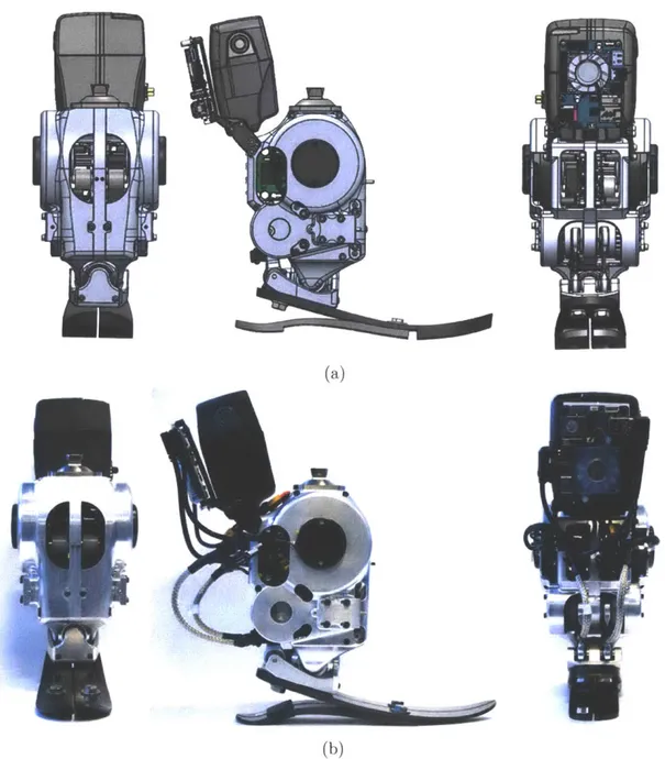
2-1 Overview of the second-iteration 2-DoF ankle. (a)Rendering (b)Physical im plem entation. . . . . 24 2-2 Key components in the transmission: (a) first-stage input pulley (12

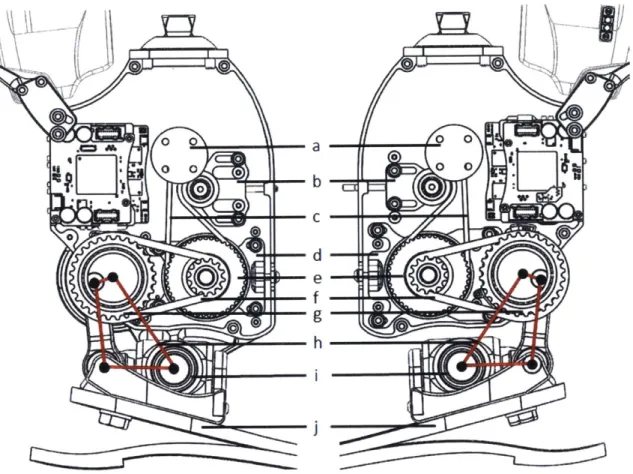
teeth) with mounting holes for the motor; (b) belt tensioner for the first-stage belt; (c) first-stage belt (3 mm pitch, 73 teeth); (d) belt tensioner for the second-stage belt; (e) first-stage to second-stage com-pound pulley (44 and 13 teeth); (f) second-stage belt (5 mm pitch, 40 teeth); (g) second-stage output pulley (28 teeth), coupled with the four-bar linkage; (h) virtual four-bar linkage that drives the foot; (i) 2-DoF joint; (j) foot prosthesis (LP Vari-Flex foot,

ossur,

Frechen, G erm any). . . . . 27

2-4 Overall transmission ratio versus sagittal plane ankle angle .. . . . . .

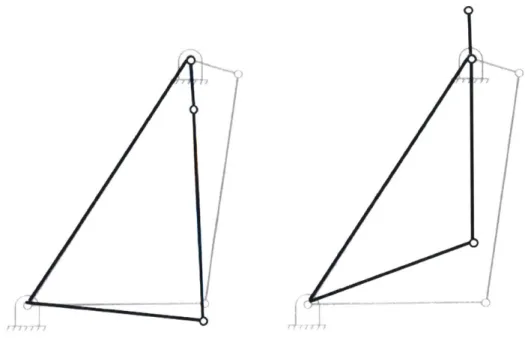
2-5 As the transmission ratio approaches infinity at the toggle positions, the system becomes non-backdrivable. . . . . 29

2-6 Physical hard stops (circled in solid red lines) were added in the second-iteration design. The hard stops were 3D printed in Nylon and backed

by the aluminum structure. Preventing the crank from moving past

the toggle positions simplifies solving the forward kinematics. . . . . . 29

2-7 Belt tensioners are on both stages. Tension can be set by adjusting the set screws. The second-stage belt is tensioned by offsetting the pulley, while the tension of the first-stage belt is set by offsetting an idler. Once the tension is set, the screws (circled in red dashed lines) must be tightened. . . . . 31

2-8 Proper flange design can not only ensure that the belts operate within the pulleys but can also prevent belt edge wear and minimize noise [19]. 33

2-9 Flanged pulleys in the ankle that were designed following the design

gu id e. . . . . 33

2-10 While the CNC milling machines are useful in making parts with com-plex geometry (such as the part on the left), cutting gears and timing pulleys require higher accuracy and repeatability. Gears and timing pulleys are typically made by CNC hobbing machines or CNC shaper cutters . . . . . 34

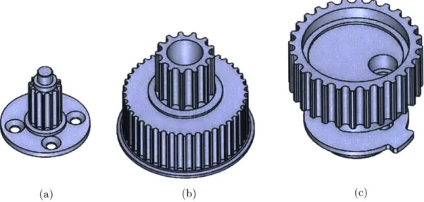
2-11 Timing pulleys in the transmission. (a) First-stage input pulley (3 mm pitch, 12 teeth). (b) First-stage output to second-stage input pulley (3 mm pitch, 44 teeth to 5 mm pitch, 13 teeth). (c) Second-stage output pulley (5 mm pitch, 28 teeth). . . . . 35

2-12 To minimize cost and reduce the effort of machining, two types of timing pulleys were designed in separate parts and press fitted together. 35

2-13 Key parameters used to calculate the pressure at the interface of the

interference fit. . . . . 36

2-14 A kinematics model of the ankle was constructed using Simulink Sim-scape Multibody to study and map forward kinematics. . . . . 38 2-15 Curve-fitting result of a 2D four-bar linkage. . . . . 39

2-16 Curve-fitting result for frontal plane motion. . . . . 40 2-17 Random motion was simulated to evaluate the fitted functions. The

simulated ground truth was compared with the motion calculated from the fitted functions. (a) Sagittal plane motion. (b) Frontal plane motion. 41 2-18 For the sagittal plane torque, the moment arm is a function of the

crank angle in the four-bar linkage. The sagittal plane torque is the sum of the torques calculated from each four-bar linkage. . . . . 42 2-19 Even at the maximum eversion and inversion positions, the connector

linkages motion on the frontal plane is negligible (smaller than 0.5 degrees). Therefore, the moment arm is approximated as a constant

(12.75 m m ). . . . . 43 2-20 The 'tendon" parts were installed with full-bridge strain gauges

(half-bridge on each side) for force and torque measurements . . . . 44 2-21 Simulation revealed that the sensing area on the part has uniform strain

distribution under load. . . . . 45 2-22 Different loads were applied in the simulation to test the linearity of

strain versus force. . . . . 46 2-23 A 'Tee Rosette" strain gauge was selected based on the aforementioned

criteria. . . . . 47 2-24 Installing strain gauges involves multiple steps, and each step must be

carefully followed. . . . . 48 2-25 Strain gauges were packaged in 3D-printed covers, and the cables were

shielded using metal-braided sleeves. . . . . 48 2-26 Setup for sensor calibration. (a) Custom fixtures were machined in 304

stainless steel. (b) Fitting the fixture in the universal test machine. (c) Test setup. . . . . 49

2-27 Calibration and curve-fitting results for (a) sensor one with R2 =

0.9998 and (b) sensor two with R2 = 0.99987 . . . . 50

3-1 Schematics of the electrical system. . . . . 52 3-2 Overall electronics system: (a) battery module, (b) power distribution

board, (c) ORDROID-XU4 single-board computer, (d) emergency stop connector, (e) absolute encoder, (f) motor, (g) FlexSEA-rigid, and (h) strain gauges. . . . . 53 3-3 Modified battery case design printed in Nylon, with a spring-loaded

button for the battery pack. . . . . 55 3-4 Custom battery module: (a) battery adapter board and (b) power

distribution and switching board. . . . . 56 3-5 Charger board designed and built for charging the battery pack that

can be charged via an ordinary Li-Po balance charger . . . . 56 3-6 Components inside the battery pack: (a) 1,600 mAh, 120 C, 22 V

Li-Po battery; (b) high-temperature silicone sealant; (c) flame-retardant silicone foam; and (d) thermally conductive high-temperature silicone foam . . . . 57

4-1 Two test fixtures were built. One is for testing and evaluating the close-loop torque controller, while the other one is for testing free space motion control: (a) Rendering ofboth fixtures; (b) Physical implemen-tation of the torque-testing fixture. . . . . 60 4-2 For the step response tests, a desired torque of 50 Nm was commanded

and repeated for 10 times. The mean and standard deviation of the 10%-90% rise time are (a) 0.0210 seconds and 0.0013 seconds, respec-tively, for motor one, and (b) 0.0193 seconds and 0.0014 seconds, re-spectively, for motor two. . . . . 62

4-3 For torque bandwidth tests, the desired torque was commanded as a 0.01 to 40 Hz chirp in 40 seconds and oscillating between -30 and 30 Nm. (a) Motor one test results. The bandwidth ranges from 28 to 37 Hz. (b) Motor two test results. The bandwidth ranges from 26 to 31 H z . . . . . 6 3 4-4 Walking trials were performed by an able-bodied person with a knee

immobilizer. The goal of the test was to evaluate torque tracking performance under body weight and to evaluate the robustness of the mechanical transmission. . . . . 64 4-5 Torque tracking results from the walking trial, averaging from all steps.

List of Tables

2.1 Design specifications. . . . . 25

Chapter 1

Introduction

1.1

Motivation

Many advances have been made in the development of bionic prostheses in the past 10 years. These so-called bionic prostheses are powered robotic devices controlled by microcontrollers, which have the capability to restore biological functions beyond conventional prostheses. Although they are much heavier than conventional ones, powered ankle-foot prostheses have been proven to improve the walking economy of transtibial amputees [1, 2, 3]. All commercially available powered ankle-foot pros-theses at present, such as Ottobock Empower [4] and

Ossur

Proprio [5] (see Figure 1-1) can only perform one degree-of-freedom (1-DoF) motions on the sagittal plane (i.e., plantarflexion and dorsiflexion). However, studies have shown that the frontal plane motions (i.e., eversion and inversion) of the ankle are associated with balance. Studies on able-body subjects found that the ankle performs active control on the frontal plane to adjust the center of pressure and maintain balance during walking [6, 7]. In addition, recent advances in peripheral neural interfaces have demonstrated the ability to preserve proprioception after lower-limb amputation, which enables ro-bust, repeatable motor control [8]. With proper robotic hardware, it is possible to fully recover the biological function of the ankle-foot complex. The above reasons emphasize the need for a powered 2-DoF ankle-foot prosthesis that is untethered, has similar weight as that of the biological ankle-foot complex, and has active control on

both sagittal and frontal plane motions. Most importantly, the ankle should generate positive net work powerful enough to support level-ground walking for an average size human. Such device does not exist yet.

(a) (b)

Figure 1: Commercially available powered ankle-foot prostheses can only perform 1-DoF motions on the sagittal plane: (a) Ottobock Empower [4] and (b) Ossur Proprio

[5].

1.2

Prior Art

Several attempts have been made to develop a powered 2-DoF ankle-foot prosthesis, as illustrated in Figure 1-2. Bellman et al. proposed a mechanical design for a high-power 2-DoF ankle for performing tasks equivalent to an able-bodied human ankle. However, the design weighs 2.1 kg, without any electronics and battery. There was also no information on how the control and electronics would look like nor test data available [9]. Ficanha et al. achieved a 2-DoF ankle prototype that is cable-driven, with electronics separate from the system. The device was able to modulate the impedance in both sagittal and frontal plane [10]. Meanwhile, Kim et al. achieved a 2-DoF prosthesis emulator that is cable-driven and can control plantarflexion and inversion-eversion torque independently [11]. Clinical trials were also performed using the same system to examine frontal plane control on balance [12]. This system is by far the only system that has been used in practice and serves as a valuable tool in

the study of biomechanics and in the search for better designs by emulating different control strategies. Conversely, as a tethered system, it is only for in-lab use.

Bowden cable termination Joint axis Medial toe Heel spring Lateral toe (a) (b) (c)

Figure 1-2: State-of-the-art powered 2-DoF prostheses: (a) System proposed by Bell-man et al. that features a mechanical design of a high-power 2-DoF ankle [9]; (b) Ficanha et al. achieved a 2-DoF ankle prototype that is cable-driven, with electronics separated from the system [10]; and (c) Kim et al.'s 2-DoF prosthesis emulator that is the only system that has been used in practice, and thus valuable in the study of biomechanics [11].

1.3

Research Objective

The objective of thesis is to build and evaluate a powered 2-DoF ankle that is unteth-ered, self-contained, and able to support level-ground walking and potentially stair ascent and descent. Such system does not exist yet.

To meet this objective, this thesis explores three research components:

" a mechanical design that can have control over frontal plane and sagittal plane motions and a robust transmission design that supports body weight and output large push-off torque during walking,

* an electronics system that is small enough to fit in the robot and a battery that has high energy density and high peak output, and

" a control system that can deliver accurate force and torque control and a con-troller that can mimic normal human walking dynamics.

1.4

Summary of Chapters

In Chapter 2, I present the mechanical design of the system. I begin this chapter by describing the design specifications of the prosthesis and the improvements made on the second iteration. I then present the kinematics model built to analyze the complex 3D motion of the proposed prosthesis. Finally, I discuss how precise force sensing can be achieved by using strain gauges.

In Chapter 3, I describe the electronics and the embedded system. I begin by in-troducing the high-level electronics system using a functional diagram and explaining the power electronics and microcontrollers used in the system. Finally, I elaborate on the design of a battery module and the associated power management circuit.

In Chapter 4, I present a control system that allows torque control and expound on how to achieve human-like walking dynamics on the prosthesis. The system's dynamics characterization and performance are also evaluated and discussed.

In Chapter 5, I discuss the contributions of this thesis and propose experiments for future research.

Chapter 2

Mechanical Design and Analysis

In this chapter, I present a second-iteration design of a 2-DoF powered ankle-foot prosthesis. The 2-DoF ankle allows for movements in the sagittal and frontal planes. I begin this chapter by describing the design specifications of the prosthesis and the improvements made on the second iteration. I then present the kinematics model built to analyze the complex 3D motion of the proposed prosthesis. Finally, I present how precise force sensing can be achieved by using strain gauges.

2.1

Overall Mechanical Design

As mentioned above, the mechanical design of the 2-DoF prosthesis in this thesis is a second iteration. The first iteration was designed and built by a former student, Luke Mooney, of the Biomechatronics Group. The design was published in a U.S. patent [13]. In this section, I compare the specifications of the two iterations and then present how the key components were redesigned.

2.1.1

Design Specifications

The design goal for both iterations is to build a 2-DoF ankle that is untethered and can support level-ground walking, stair ascent and descent, and uneven terrains for an average-sized human (75 kg, 175 cm). Locomotion data from the literature were used

[14, 15, 16]. The second iteration, displayed in Figure 2-1, has a larger joint range of motion, more robust transmission (see Section 2.1.2), and more powerful battery

(see Section 3.4) but is larger in size and heavier in weight. All the metal parts were made in 7075-T6 aluminum. Detailed design specifications of the two iterations are listed in Table 2.1.

(a)

(b) (b)

Figure 2-1: Overview of the second-iteration 2-DoF ankle. (a)Rendering (b)Physical implementation.

Table 2.1: Design specifications.

Parameter First Iteration Second Iteration

Weight without Battery (kg) 2.08 2.42

Battery Weight (kg) 0.26 0.33

Height" (mm) 210.8 210.8

Width (mm) 110.0 126.6

Max. Allowable Inversion (deg) 11 13.5

Max. Allowable Eversion (deg) 11 13.5

Max. Allowable Dorsiflexion (deg) 7 9 Max. Allowable Plantarflexion (deg) 18 21

Transmission Ratiob 67 ± 33 57 ± 28

Peak PF-DF* Torque (Nm)c 109 162.4

Peak INV-EV* Torque (Nm) 34.81 59.35

Battery Voltage (V) 22.2 22.2

Peak Current (A)

33.75d

50e

Motor Torque Constant (Nm/A) 0.095 0.112

Torque Bandwidth (Hz) 26

a. From the bottom of foot prosthesis (without cosmesis) to the bottom of pyramid adapter.

b. For most of the range of motion. See Section 2.1.2 for more detail.

c. Assuming a transmission ratio of 34:1 for iteration one and 29:1 for iteration two.

d. Limited by battery (22.2 V, 1350 mAh, 25 C).

e. Limited by on-board ceramic fuses (25 A on each motor driver).

-: Not available.

*PF-DF: Plantarflexion-Dorsiflexion; INV-EV: Inversion-Eversion.

As presented in Table 2.1, the major difference between the two iterations is the peak torques, due to the limitation from the battery. A 22.2 V lithium-polymer (Li-Po) battery module from a commercial powered ankle prosthesis (BiOM, BionX, now part of Ottobock, Cambridge, MA, USA) was retrofitted for used in the first-iteration 2-DoF ankle, which has a 1,350 mAh capacity and a discharge rate of 25C. In addition, a 15 A ceramic fuse is located inside the battery module. Therefore, to achieve the peak current of 33.75 A (1.35x25), the fuse must be removed, which can be dangerous. As a result, a new battery module (22.2 V, 1,600 mAh, 120 C) was built for the second-iteration ankle (see Section 3.4 for more detail). For the second-iteration 2-DoF ankle, a 25A ceramic fuse is placed on each motor driver board, resulting in

a current draw of 50 A from the battery during peak, while the battery itself peaks at 192 A. Note that the first-iteration ankle can output high torques similar to the second-iteration ankle, but this would require a power supply or a different battery. The new battery pack does not fit in the first-iteration ankle.

2.1.2

Transmission Design

For the transmission design, the second-iteration ankle follows the same concept as its predecessor, which uses two brushless electric motors (U8 Lite KV85, T-motor, Nanchang, Jiangxi, China) to form a differential drive: when the two motors are moving in sync, the ankle performs only sagittal plane motion, and when the motors are not moving in sync, the ankle performs coupled frontal and sagittal plane motion (see Section 2.2 for more detail). Each motor features two-stage belt drive coupled to a four-bar linkage, which drives the foot. Figure 2-2 illustrates the key components of the transmission design.

The four-bar linkage in the transmission introduces a variable transmission ratio. Figure 2-3 illustrates a more detailed representation of the four-bar linkage depicted in Figure 2-2. A planar four-bar linkage is a well-studied mechanism [17]. The transmission ratio, or mechanical advantage, from the input crank torque Tin to output rocker torque Tot can be solved via the principle of virtual work [18]:

Te=

ToutV/

(2.1)

where

T_ t _ (-abcosO sin0 - bg sin $ + abcos 0 sin V)

R = -=-=(2.2)

Tin (ag sin0

+

abcos@ sin9 - abcos0 sinp)

Using Equation 2.2, the overall transmission ratio (including the contribution from the belt drive) versus the ankle angle in the sagittal plane can be derived, as illustrated in Figure 2-4. Note that as the joint moves toward the limit positions, the transmission ratio reaches infinity; this is known as the "toggle positions" in the four-bar mechanism [17], as displayed in Figure 2-5. At the toggle positions, the

0 00

0

d

e

f

h

Figure 2-2: Key components in the transmission: (a) first-stage input pulley (12 teeth) with mounting holes for the motor; (b) belt tensioner for the first-stage belt; (c) first-stage belt (3 mm pitch, 73 teeth); (d) belt tensioner for the second-stage belt; (e) first-stage to second-stage compound pulley (44 and 13 teeth); (f) second-stage belt (5 mm pitch, 40 teeth); (g) second-stage output pulley (28 teeth), coupled with the four-bar linkage; (h) virtual four-bar linkage that drives the foot; (i) 2-DoF joint;

(j) foot prosthesis (LP Vari-Flex foot, Ossur, Frechen, Germany).

ankle is not backdrivable. The second-iteration 2-DoF added physical hard stops at the toggle positions to prevent the crank from moving beyond those toggle positions, as presented in Figure 2-6. Restricting the crank motion in the desired range (180 degrees) simplifies solving the forward kinematics, as there exists a one-to-one rela-tionship between crank and rocker angles. In other words, if the crank is able to pass the toggle positions, then the same rocker position can result in two different crank positions, making it difficult to map the forward kinematics.

The hard stops displayed in Figure 2-6 were 3D printed in Nylon (PA11 Black)

run 0 0 0

CE

0

a

b

C

Dorsiflexision

Plantarflexision

Crank (pulley)

aI=95 L .*

Base

9=56.4mm

h

b =35.5mm

/ # Rocker (foot)

Connector

=44mm

90 80 70 60 50 40 30 20 10 0

Figure 2-3: The four-bar linkage in the transmission.

-Dorsiflexion Plantarflexion

-I

I

'I

-9 -6 -3 0 3 6 9 12 15 18 21 Sagittal Plane Ankle Angle (degree)

Figure 2-4: Overall transmission ratio versus sagittal plane ankle angle.

mm" 0 0 U, U,

E

U, C U, I-

F-,~

lit)

Figure 2-5: As the transmission ratio a system becomes non-backdrivable.

pproaches infinity at the toggle positions, the

Figure 2-6: Physical hard stops (circled in solid red lines) were added in the second-iteration design. The hard stops were 3D printed in Nylon and backed by the alu-minum structure. Preventing the crank from moving past the toggle positions sim-plifies solving the forward kinematics.

(5

and backed by the aluminum structure. The Nylon hard stops provide a 10-degree cushion for the cranks beyond the toggle positions before they would hit the main aluminum structure. Software hard stops were also implemented as unidirectional springs.

2.1.3

Timing Belt Drive Design

One of the most critical issues with the first-iteration ankle concerned the timing belt drive design: when the ankle experienced high torque, the belt would "jump tooth." Several factors can contribute to the jumping of teeth. Therefore, in the second iteration, the timing belt drive was redesigned, and some improvements were made to prevent jump tooth, in addition to increasing the overall performance:

" Using more advanced belts.

* Adding belt tensioners.

" Ensure sufficient teeth are in mesh with pulleys.

" Ensure sufficient belt width and pulley width.

* Better pulley flange design.

These design changes were made by following a design guide [19]. In the second it-eration, the PowerGrip GT3 timing belts (Stock Drive Products/Sterling Instrument, Hicksville, NY, USA) were used in both stages of the belt drives (3 mm pitch, 15 mm wide, 73 teeth for the first stage and 5 mm pitch, 15 mm wide, 40 teeth for the sec-ond stage). The GT3 belts have higher load-carrying capacity (hence improved tooth jump resistance), lower noise, less backlash, and superior durability compared with the older PowerGrip HTD belts. Belt tensioners were included in the second-iteration design to enable not only proper belt tension and transmission but also easier assem-bly. Installing belts in the first-iteration ankle was a difficult task because the pulley positions were fixed. Therefore, the belts needed to be over-stretched to fit in the pulleys.

________ -I

Figure 2-7 illustrates how to adjust belt tension on the second-iteration ankle. The tension of the second-stage belt must first be set by two set screws, which moves the second-stage input pulley and adjusts the center distance between the input and output pulleys. Once the tension is set, the four screws on the mounting plate must be tightened. The tension of the first-stage belt can then be set by another set screw, with two tightening screws. The tensioner of the first-stage belt is a backside idler with a 19 mm diameter, as recommended by the design guide. The range of motion of both tensioners was designed to be capable of stretching the belts by one pitch (3 nin for the first stage and 5 mi for the second stage).

...

0)

'o.

Figure 2-7: Belt tensioners are on both stages. Tension can be set by adjusting the set screws. The second-stage belt is tensioned by offsetting the pulley, while the tension of the first-stage belt is set by offsetting an idler. Once the tension is set, the screws (circled in red dashed lines) must be tightened.

Another benefit to having belt tensioners as idlers in the first-stage belts is to increase the number of teeth in mesh with the pulleys. According to the design guide, to ensure proper torque transmission, the belt should have at least six teeth in mesh with the pulley. Following the design guide, the first-stage belt was designed to

have six teeth in mesh with the input pulley under the default tension. As the idler gets closer, the number of teeth in mesh further increases, as illustrated in Figure 2-7. Belt width also is a critical factor in tooth jump resistance, as wider belts and pul-leys have more contact area, and hence more friction, to resist tooth jump. According to the experimental data from the design guide, under normal installation tension, the minimum torques that cause tooth jump on a 3 mm pitch, 6 mm wide and a 5 mm pitch, 15 mm wide PowerGrip GT3 belt are 3.95 Nm and 35.93 Nm, respectively. In the experiment, the 3 mm pitch belt was installed on a 30-tooth pulley, while the 5 mm pitch belt was installed on a 20-tooth pulley. Estimating based on these data, the minimum tension per unit belt width that can cause tooth jump for a 3 mm and 5mm pitch GT3 belt are approximately 45.97 N/mm and 150.46 N/mm. Since the second-iteration ankle uses 15 mm wide belts for both stages, the maximum allowable

belt tension is then 689.55 N and 2,256.9 N, respectively, for each stage. Note that when the motor is at peak torque, the tension on the belts is 448 N for the first stage and 992 N for the second stage. Therefore, safety factors of 1.41 and 2.27 are on each stage of transmission.

Pulley guide flanges also were redesigned in the second-iteration ankle, following the design guide. Flanges are essential in keeping the belts operating on the pulleys. In addition, proper flange design can not only restrain belts on the pulleys but also prevent belt edge wear and minimize noise. For two pulley drives, it is suggested that flanges should be added on both sides of the pulleys, or each pulley should have flanges on the opposite sides. Figure 2-8 illustrated the flange geometry. The dimension of each term is listed in Table 2.2 [19]. Figure 2-9 displays the design of the flanged pulleys in the ankle. Note that the flange height for the pulley on the right (motor input pulley) is only 1.35 mm, which is 0.35 mm smaller than the minimum required height. This dimension was limited to fit the mounting holes of the motor.

2.1.4

Timing Belt Pulley Manufacturing

The first-iteration ankle used a computer numerical control (CNC) mill to machine the pulleys, which could be one of the factors that contributed to tooth jump. The

16I 8 Nominal No sharp corners Fia _/ NOW

/1

ke M~ovet

Figure 2-8: Proper flange design can not only ensure that the belts operate within

the pulleys but can also prevent belt edge wear and minimize noise [19].

Table 2.2: Dimensions for pulley flanges [19].

Belt Type

Minimum Flange Height (mm)

Face Widtha (mm)

3mm GT3

1.70

+1.25

5mm GT3

2.20

+1.50

a. Additional to the belt width.

17

"IN1IIIII if I

in'

.... m~~m~m~~m mmu --- -q

-.

1-.9-7-L1m

m GT3

I

Figure 2-9: Flanged pulleys in the ankle that were designed following the design

guide.

Face Wkkh

5mm GT3

tooth profile of a pulley is critical to the performance of the belt drive, as it directly

affects the mesh quality between the belt and pulley. While CNC milling machines

are useful in creating parts with complex, irregular geometry, they are not suitable

for cutting gears and pulleys, which requires high accuracy and consistency (Figure

2-10). Although a high-end CNC milling machine with the proper setup can achieve

those requirements, it is unpractical, and the price can be prohibitive.

Timing belt pulleys and gears are typically constructed via hobbing, shaper

cut-ting, or broaching. These processes use the cutting tool specific to the desired tooth

profile, resulting in high repeatability and accuracy. The timing pulley hobbing and

shaper cutting machines can maintain a tolerance within 0.00254 mm (0.0001 inch)

[20], while the tolerance of a typical CNC milling machine is approximately

+/-

0.13

mm (0.005 inch) [21].

Figure 2-10: While the CNC milling machines are useful in making parts with complex

geometry (such as the part on the left), cutting gears and timing pulleys require

higher accuracy and repeatability. Gears and timing pulleys are typically made by

CNC hobbing machines or CNC shaper cutters.

Three different timing pulleys are in the transmission, as depicted in Figure

2-2. Figure 2-11 provides a more detailed view of each pulley. To minimize cost and

reduce the effort of machining, the pulleys in Figure 2-11 (a) and (b) were designed

in separate parts and were press fitted together, as illustrated in Figure 2-12.

(b)

Figure 2-11: Timing pulleys in the transmission. (a) First-stage input pulley (3 mm pitch, 12 teeth). (b) First-stage output to second-stage input pulley (3 mm pitch, 44 teeth to 5 mm pitch, 13 teeth). (c) Second-stage output pulley (5 mm pitch, 28 teeth).

o

Figure 2-12: To minimize cost and reduce the effort of machining, two types of timing pulleys were designed in separate parts and press fitted together.

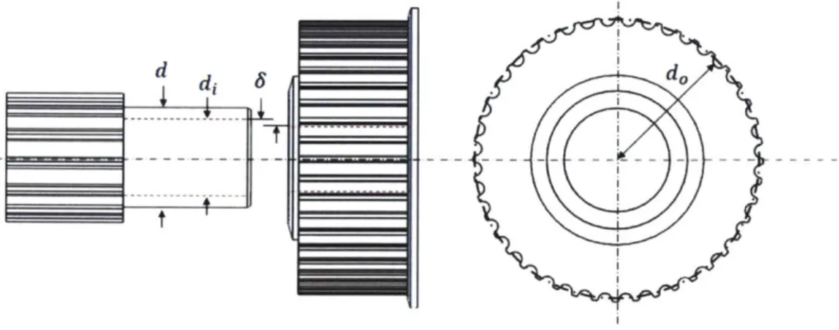
Friction analysis on the parts was performed to ensure that the press-fit pulleys can transmit the torque without slipping. The friction force of the interference fit is estimated by first calculating the pressure p generated at the interface [22]:

3

P

=

j(2.3)

where d is the nominal shaft diameter, di is the inside diameter of the shaft (if

any), do is the outside diameter of the hub,

is the diametral interference between

the shaft and hub (6

= dshaft - dhu),

E is Young's modulus, v is Poisson's ratio, with

subscripts o and i representing the hub and shaft, respectively. If the hub and shaft

are of the same material, then Equation 2.3 can be simplified as follows

[22]:

E3 [(d2 -

2

)(d

2

_d)

_(2.4)

2d3 d2 -2 4

Figure 2-13 presents the geometric relationships of each parameter, using one of

the pulleys as an example:

d _d.

-w

Figure 2-13: Key parameters used to calculate the pressure at the interface of the

interference fit.

With the pressure calculated, the friction force Ff at the interface of the

interfer-ence fit can be estimated [22]:

F5 = f N =

f

(pA) =

f

[p27r (d/2) 1| =

fprdl

(2.5)

where N is the normal force acting at the interface, 1 is the length of the hub, and

f

is the coefficient of the friction of the material. Finally, the torque capacity T can

36

199 t I

be calculated as the friction force times the moment arm d/2 [22]:

T = Ffd/2 =

fprdl

(d/2) = (r/2)

fpd

2 _(2.6)

Using Equations 2.4 and 2.6 with the material data (7075-T6 aluminum) taken from the literature [23], the pulley in Figure 2-11 (a) was designed to have a torque capacity between 43.49 Nm and 65.08 Nm, while the pulley in Figure 2-11 (b) was designed to have a torque capacity between 107.11 Nm and 268.45 Nm. The numbers vary because machining tolerance was considered, with a safety factor of around 12 at the lower tolerance and 25 at the upper tolerance. Detailed drawings of the pulleys are available in Appendix A.

2.2

Kinematics Model

As mentioned in Section 2.1.2, the ankle transmission is a type of differential drive, formed by two sets of the four-bar linkage connected to a base (foot). That is, the ankle is a 3D closed-chain mechanism. It is well known that an analytical solution to the forward kinematics of a spatial closed-chain mechanism can be difficult, sometimes impossible, to solve. Even if an analytical solution is achieved, it would be resource intensive for the embedded system. Therefore, in this section, I present how to simulate the system and map the forward kinematics in a virtual environment, in addition to how to find the moment arms.

2.2.1

An RR-2RSS Mechanism

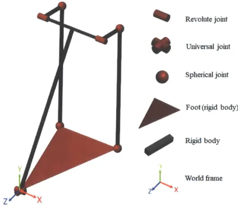
A kinematics model of the ankle was constructed in a virtual environment using MATLAB/Simulink Simscape Multibody (MathWorks Inc, Natick, MA, USA), as illustrated in Figure 2-14. The model simulates a RR-2RSS mechanism, where R represents a revolute joint, and S represents a spherical joint. A universal joint is formed by two revolute joints with mutually orthogonal axes and coincident origins. The world frame is a motionless, orthogonal, right-handed frame and serves as the

-- -_ - --- - -- - -- ~~*1 ground of all the frame networks in the model. The spherical joints model the swivel

bearings in the ankle, which have a 27-degree range of motion on the z-axis (hence a 13.5-degree inversion/eversion). Revolute joint

p

0

Universal joint Spherical joint

P

W

Foot(rigid body) - Rigid body Y World frame

Figure 2-14: A kinematics model of the ankle was constructed using Simulink Sim-scape Multibody to study and map forward kinematics.

2.2.2

Mapping Forward Kinematics

As mentioned in Section 2.1.2, the crank motion in the four-bar linkage is constrained by hard stops, providing a one-to-one relationship between the crank and rocker position. To determine the sagittal plane joint angle, the kinematics of a 2D four-bar linkage was first simulated and fitted using the

fit()

command in MATLAB. The curve fitting was performed by non-linear least squares and a two-term Fourier series as base, which has the following form:

Z/

r(6) = ao

+

a1 cos(w9)

+

b1 sin(wO)

+

a2cos(2w9)

+

b2sin(2w)

where r() is the rocker angle, and 0 is the crank angle. The parameters ao, ai, a2,

bi, b2, and w were determined by the curve-fitting function. Figure 2-15 displays the

fit result. The fitted curve has a root-mean-square error (RMSE) of 0.009 degrees.

C, 25 20 15 10 5 0 -5 -10 -60 -40 -20 0 20 40 60 80 100 120

Crank Angle (degree)

Figure 2-15: Curve-fitting result of a 2D four-bar linkage.

Note that this works only for a 2D four-bar linkage. When the two motors are not moving in sync, the ankle performs coupled frontal and sagittal plane motion. However, the sagittal plane motion <k can be easily estimated as the average position of the two rockers: <D = [r1 (01)

+

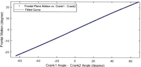
r2(92)] /2. Frontal plane motion also was also fitted

using the same method. The fit result is dipicted in Figure 2-16. Note it is assumed that the frontal plane motion is a function of the crank 1 angle minus the crank 2

angle. The fit has a RMSE of 6.446x105 degrees.

To test the fits, random motion was simulated. The simulated ground truth was compared with the motion calculated from the fitted functions, as illustrated in Figure 2-17. The RMSE is 0.1426 degrees for sagittal plane motion, and 0.3776 degrees for frontal plane motion.

Rocker Angle vs. Crank Angle

- Filled Curve

20 Frontal Plane Motbon vs. Crankl - Crank2 F ied Curve )10 0 0 -10 -20 40 40 -20 0 20 40 60

Crank1 Angle - Crank2 Angle (degree)

Figure 2-16: Curve-fitting result for frontal plane motion.

2.2.3

Moment Arm Calculation

Force sensors were installed on the connectors of the four-bar linkage (see Section 2.3

for more detail). Therefore, both sagittal and frontal plane torque can be calculated

as the measured force times the moment arm. For the sagittal plane, the moment

arm is a function of the crank angle in the four-bar linkage, as illustrated in Figure

2.7. The sagittal plane torque is the sum of the torques calculated from each four-bar

linkage.

In Figure 2-18, Oo represetns the crank angle when the rocker (foot) is at the zero

position (101.73 degrees), and

4

_{represents the angle relative to that zero position.}

To find the moment arm 1, first calculate c using the law of cosines:

c = Va2 + g2 - 2ag cos (o

+)

(2.8)

Then, set s = (c

+

h

+

b) /2. Using Heron's formula,

S= (2 s(s - a)(s - b)(s - c)) /h (2.9)

For frontal plane torque, even at the maximum eversion and inversion positions, the connector linkages motion on the frontal plane is negligible (smaller than 0.5

0 1000 2000 3000 4000 5000 6000 7000 8000 9000 10000 Time (msec) (a) 0 1000 2000 3000 4000 5000 Time (mse (b) 6000 7000 8000 9000 10000

Figure 2-17: Random motion was simulated to evaluate the fitted functions. The simulated ground truth was compared with the motion calculated from the fitted functions. (a) Sagittal plane motion. (b) Frontal plane motion.

degrees), as illustrated in Figure 2-19. Therefore, the moment arm is approximated as a constant (12.75 mm).

2.3

Force Sensing

In the first iteration of the ankle, force sensing was performed by measuring the motor current and was then converted to joint torque through joint geometry. However, due

20 15 10

-Sinuated Ground Truth .--- Caciuated fromn Filled Functio

8

5 0 -5 -10 15 101

Simtedated Ground Truth |----Caeuaed from Fitted Function

-nlildrwdrt 5 0 -5 -10 C 0 0 LL -15

Crank (pulley)

a

C _Connector BaseQ

h

Y

Rocker (foot)

b

Moment arm

I

Figure 2-18: For the sagittal plane torque, the moment arm is a function of the crank angle in the four-bar linkage. The sagittal plane torque is the sum of the torques calculated from each four-bar linkage.

to high reflected inertia in the transmission, it is difficult to sense force accurately with motor current, especially when external loads are applied, as external loads might not spin the motor at all. Here, I present how to precisely measure forces and joint torques using strain gauges.

2.3.1

Full-Bridge Strain Gauge

Full-bridge strain gauges were installed on the "tendon" parts (half-bridge on each side), which is the connector of the four-bar linkage, for force measurement, as illus-trated in Figure 2-20. Joint torques can then be easily calculated with moment arms

(see Section 2.2.3 for more detail).

This full-bridge configuration was selected because it can measure axial strain and has much better sensitivity than half-bridge and quarter-bridge configurations.

12.5 mm

Figure 2-19: Even at the maximum eversion and inversion positions, the connector linkages motion on the frontal plane is negligible (smaller than 0.5 degrees). Therefore, the moment arm is approximated as a constant (12.75 mm).

In addition, this full-bridge configuration compensates for the Poisson effect and minimizies the effects of temperature [24].

2.3.2

Strain Gauge Selection

Before selecting the correct strain gauge to use, the tendon part was tested in simu-lation to ensure the sensing area has even strain distribution under load, as displayed in Figure 2-21.

In the simulation, the pulling force was set to 1,600 N, the peak force that will be applied on the part. The strain under this peak force is approximately 0.08%. In addition, different forces were simulated to test the linearity of strain versus pulling force, as depicted in Figure 2-22.

As the simulation results revealed that the tendon part is ideal for force sensing, I selected the strain gauge according to the following criteria:

Figure 2-20: The 'tendon" parts were installed with full-bridge strain gauges (half-bridge on each side) for force and torque measurements.

" Size

" Strain range

" Ease of installation

" Grid resistance

" Gauge pattern

Each criterion is critical for the strain gauges to function properly. The size of the gauges should be as large as possible for ease of installation but still fit in the sensing area. The grid resistance should be as large as possible to reduce dissipation due to current consumption. Moreover, the strain range should be greater than the maximum strain that will appear on the part. Finally, the gauge pattern should ideally be one single gauge with a half-bridge circuit, in which the two grids are orthogonal to each other.

Based on the requirements above, a 'Tee Rosette" strain gauge (MMF307425, Micro-Measurements, Raleigh, NC, USA) was selected, which features orthogonal

R,

R3 R2 R

R,

R4 + Vo R2 R3 VE: 5V Vo : Output to microcontroller RI, R2. R3. R4: Strain gauges

t1.6kN

ESTRN

I

8.240e-004 7.554e-004 6"69e-004 &184em 5.4We004 4813e4D4 4.127e-004 3.442e.004 2.756e 4 201le-404 1.385e-W4 6.999e-0S 1A42e.D6

Figure 2-21: Simulation revealed that the sensing area on the part has uniform strain distribution under load.

grid patterns and has a 3% strain range, 350 Ohm resistance, and pre-attached ribbon leads and cable wires, as displayed in Figure 2-23.

2.3.3

Installation and Packaging

The performance of strain gauges is greatly affected by the installation process and packaging. To ensure proper installation, an installation kit (MMF307425, Micro-Measurements, Raleigh, NC, USA) from the vendor was used. The installation in-volved the following major steps [25]:

" Surface preparation

" Positioning

* Apply adhesive " Curing

0'

0 1 2 3 4 5

strain (m/m)

6 7 8

Figure 2-22: Different loads were applied in the simulation to test the linearity of

strain versus force.

For surface preparation, the part was first degreased with solvents and abraded

with conditioner, which helps the adhesive to bond better. Afterward, the gauge

was positioned using Mylar tape, which can be easily peeled off from the gauge and

does not interact with the adhesive. The adhesive is a special epoxy that ensures

permanent bonding. After applying the adhesive, the gauge must be clamped for at

least six hours. Finally, a protective polyurethane coating was applied. Figure 2-24

displayed the finished part.

As illustrated in Figure 2-24, the pre-attached ribbon leads on the strain gauges

are extremely thin (32 AWG). This serves to save space and minimize the strain

field around the gauges. However, these thin leads are prone to breaking under

dynamic environments. To protect the leads, I applied silicone rubber (3140 RTV,

Dow Corning, Midland, MI, USA) around them. The selected silicone rubber is

non-conductive, self-leveling, and has a high elongation of 420%.

Finally, protective covers were designed and 3D printed to package the strain

gauges and parts. The wires were packaged in metal-braided sleeves, which were

1600 1400

.

0 1200 1000 800 600 400 200 9 - 101 • force-strain data f(x)=1941747.5728x+-4.9487e-14

10.16mm

Figure 2-23: A 'Tee Rosette" strain gauge was selected based on the aforementioned criteria.

connected to the ground of the microcontrollers for shielding (minimizing noise), as displayed in Figure 2-25.

2.3.4

Calibration

Both sensors in Figure 2-25 were calibrated using a universal testing machine (5984, INSTRON, Norwood, MA, USA). Custom fixtures were designed and machined to hold the parts in the universal testing machine. The fixtures were machined in 304 stainless steel so that they would not yield prior to the test parts, which were made in 7075 aluminum. Figure 2-26 displays the fixture design and test setup.

During the test, the sensors were pulled and compressed at 200 N intervals un-til 2,000 N was achieved. The sensor readings were logged by the control board (FlexSEA-Rigid, Dephy, Boston, MA, USA), which has a cascaded RC low-pass filter (cutoff at 1.6 kHz) and a dual-stage, high common-mode rejection ratio (CMRR) instrumentation amplifier with the gain set to 202.6.

The test and curve fitting results are depicted in Figure 2-27, which suggest an nearly linear relationship between external forces and sensor readings.

Figure 2-24: Installing strain gauges involves multiple steps, and each step must be carefully followed.

Figure 2-25: Strain gauges were packaged in 3D-printed covers, and the cables were shielded using metal-braided sleeves.

(a) (b) (c)

Figure 2-26: Setup for sensor calibration. (a) Custom fixtures were machined in 304 stainless steel. (b) Fitting the fixture in the universal test machine. (c) Test setup.

1•strain

gauge data 1500

---

f(x)=-1289.5927x+12.0596 1000 500 R2 =0.9998

zK

0 0 IL -500 -1000 -1500 -2000 -1.5 -1 -0.5 0 0.5 1 1.5

Strain Gauge Reading (V)

(a)

Sstrain gauge data

f(x)-1360.8316x+-0.329971 1000 z 500R 2 =0.99987 0 -500 -1000 -1500 -2000 -1.5 -1 -0.5 0 0,5 1 1.5

Strain Gauge Reading (V)

(b)

Figure 2-27: Calibration and curve-fitting results for (a) sensor one with R2_{= 0.9998}

Chapter 3

Electronics and Embedded System

This chapter presents the electronics hardware used in the 2-DoF ankle, including the low-level motor drivers, mid-level embedded controllers, high-level computing plat-form, sensors, and battery. I begin this chapter by introducing the overall electronics system using a functional diagram and providing a brief description of each compo-nent. Finally, I present the custom battery module that was built to power the whole system.

3.1

System Overview

Figure 3-1 illustrates the overall electronics system of the 2-DoF ankle. The whole system is powered by a battery module that contains a 6-cell 22 V Li-Po battery. The system has a custom-made power distribution board that has a step-down volt-age regulator (D24V50F5, Pololu, Las Vegas, NV, USA) on it to convert the 22 V to 5 V (5 A maximum) to power the ODROID-XU4 single board computer

(HARD-KERNAL, AnYang, GyeongGi, South Korea). The ODROID-XU4 runs high-level

control algorithms and communicates with two FlexSEA-rigid boards (Dephy,

MAY-NARD, MA, USA) using serial bus. FlexSEA-rigid boards are mid-level and low-level

controllers that take sensor readings, which include the strain gauge, encoder, and perform control on joint position and joint torque. A 14-bit absolute motor encoder

position. A heavy-duty emergency stop (ED250, Albright International, Hampshire,

UK) can be connected to the power board for emergency shut down. This emergency

stop is optional and can be taken off and replaced by a shorted connector. Figure 3-2

illustrates a physical model of each component in the electronics system.

22V Battery -Power Switch Module Emergency Stop

I (Optiona)

Power - -Distribution

Board

5 V, 5A max.

22V,25A max 22V.25A max.

ODROID-XU4

FlexSEA-Rigid FlexSEA-Rigid

Strain Gauge Encoder Motor Strain Gauge E er Motor

Figure 3-1: Schematics of the electrical system.

3.2

Power Electronics and Microcontrollers

The FlexSEA-rigid board originates from the Flexible, Scalable Electronics

Architec-ture (FlexSEA), an open-source brushless drive and motor controller developed for

wearable robotic applications [26]. FlexSEA-rigid is a single-package solution that

integrates the features of four individual boards. The design consists of four logical

blocks named Regulate, Manage, Execute, and Communicate. The Manage module

is centered around a powerful microcontroller (Cortex-M4, ARM, Cambridge, UK). It

e

f

h

Figure 3-2: Overall electronics system: (a) battery module, (b) power distribution board, (c) ORDROID-XU4 single-board computer, (d) emergency stop connector, (e)

absolute encoder, (f) motor, (g) FlexSEA-rigid, and (h) strain gauges.

hosts mid-level control algorithms, which can be programmed by the developers. The Execute module controls the brushless motor; it runs fast, low-level controllers based on the state requested by Manage. Feedback loops are closed within the brushless drive at 1 kHz and 10 kHz for position and current, respectively. Meanwhile, the Regulate module supervises Manage and Execute. It contains on/off logic and sen-sors to monitor experiments and board state. The Communicate module groups all of the communication peripherals in FlexSEA-rigid. Wired interfaces include one USB port and one RS-485 interface. Wireless capability can be achieved by connecting a

pre-certified Bluetooth module (RN-42, Microchip, Chandler, Arizona, USA). Other peripherals are available on the expansion connector [27].

3.3

Real-Time Computer

The ODROID-XU4 single-board computer is a computing device with more power-ful, more energy-efficient hardware and a smaller form factor compared to the pop-ular Raspberry Pi single-board computer [28]. The ODROID-XU4 on the 2-DoF ankle runs the Ubuntu operating system with a Linux time kernel 3. The real-time kernel was integrated by Tony Shu, who is currently a graduate student at the Biomechatronics Group of MIT Media Lab. He also developed the software communi-cation stack between the ODROID-XU4 and the FlexSEA-rigid boards and set up the software development environment in the computer. The communication stack uti-lized multithreading technique and can communicate with each FlexSEA-rigid board at 2,000 Hz.

3.4

Battery Module Development

Custom battery module was built and integrated into the 2-DoF ankle. The design of the battery case was modified from the one on the BiOM commercial powered ankle and was 3D printed in Nylon (PA 11 Black). Using the same design, the battery pack has a spring-loaded button for it to latch in the battery box. The angle of the battery is adjustable to prevent it from hitting the shank of the wearer. Figure 3-3 illustrates the mechanical design of the battery module.

As mentioned in Section 3.1, custom circuit boards were designed and built for the battery module, as illustrated in Figure 3-4. The power adapter board shown in Figure 3-4 (a) transmits the battery power and voltage of each cell through a connector, while the power distribution board in Figure 3-4 (b) converts the battery voltage from 22 V to 5 V to power the ODROID. The 22 V power is sent to two FleaSEA-rigid boards through the emergency stop connector. When the emergency

Figure 3-3: Modified battery case design printed in Nylon, with a spring-loaded button for the battery pack.

stop is not in use, the connector is shorted. Besides distributing power and converting voltage, there is also a timing circuit in the power distribution board to ensure that the battery can power the two FleaSEA-rigid boards and the ODROID computer at the same time with a single-pole, single-throw rocker switch.

Another custom board was designed and built for charging the battery (see Fig-ure 3-5). With this charging board, the battery pack can be charged via an ordinary Li-Po balance charger. Figure 3-6 displays the components inside the battery pack. The battery used is a 1,600 mAh, 120 C, 22 V Li-Po battery. To protect the battery, the power connection pads were covered with high-temperature silicone sealant. The battery is fixed in place by flame-retardant silicone foams. Notably, there is a ther-mally conductive high-temperature silicone foam between the battery adapter board