The death knells of mature technologies

I

IT

m

HD28

The

International

Center

for Research

on

the

Management

of

Technology

The

Death

Knells

of

Mature

Technologies

Carl W.I. Pistorius*

James

M.

Utterback

February

1995

WP

#

135-95

Sloan

WP

#

3859-95

''Institute for

Technological

Innovation

University of Pretoria

Will

appear

in

Technological

Forecasting

and

Social

Change

©

1995

Massachusetts

Institute of

Technology

Sloan School

of

Management

Massachusetts

Institute of

Technology

38

Memorial

Drive,

E56-390

MASSACHUSETTSINSTITUTE

OFTECHNOLOGY

:T

271995

LIBRARIES

ABSTRACT

The

oscillatory' behavior in the

mature

phase

of

some

technologies' diffusion-related S-curves

are investigated, specifically with regard to the influences that other technologies can

have on

the oscillations

The

notion

of

mortality indicators is raised, i.e.

whether

such behavior is a

signal that the

mature technology

is

under

attack

from

an

emerging technology

The

case of

structural panels in the

wood

products industry is considered as an example,

and

an

updated

forecast

of

the substitution

of

oriented strand

board

for

plywood

is

made

It is

concluded

that

factors such as

macroeconomic

business cycles are primarily responsible for the oscillations in

plywood's

S-curve, although it is

argued

that an

emerging technology

can also contribute to

perturbations in a

mature

technology's S-curve.

Two

possible alternative explanations for the

oscillatory behavior are also discussed, viz a previously

proposed

chaos-formulation and a

mathematical

model

based

on

modified Lotka-Volterra equations This

model

shows

that

oscillatory behavior in

mature

technologies' S-curves can also result

from

symbiotic

interaction

between

two

technologies

under

certain circumstances

Introduction

Oscillatory behavior in the

mature

phase of the diffusion-related S-curves

of

technologies is a

phenomenon

that has

been

recognized

and

discussed in the literature.

One

of

the reasons

why

this type ot oscillatory behavior is

of

more

than passing

academic

interest, is the question

whether

the oscillations signal the

demise

of the

mature

technologies, ie

whether

thev are

mortality indicators foi

mature

technologies, as has been

proposed

previously in the literature

technologies, but also in the

development

and execution oi'

end-game

strategies for

mature

technologies In this paper

we

address the question

whether

the oscillations are indeed

mortalitv indicators, or in the general case,

whether

they are in

some

\\a\ triggered b\ the

interaction with another technology

Although

this paper

does

not attempt to speak the final

word

on

the subject, it adds to the debate by considering

two

cases

In the first case, that of

plywood

being "attacked" by oriented strand board

(OSB)/waferboard.

it is

shown

that the oscillatory behavior in

plywood's

S-curye correlates

very well with the fluctuations in the residential fixed investment pattern in the

US,

and it is

concluded

that this

macroeconomic

effect rather than the

emergence

of

OSB

causes the

oscillations in

plywood's

S-curve This leads to the conclusion that oscillatory behavior per se

is not a mortality indicator in the sense described

above

However,

it is possible to identify

some

perturbations in the S-curve that can be ascribed to the

emergence

of

a

new

technology

In the

second

case, a conceptual

model

is

developed

to illustrate the

more

general case of

interaction of

one

technology with another

Other

authors

have argued

that the oscillatory'

behavior in the

mature

phase ofan S-curve

may

be a chaotic effect

However,

these

arguments

have not taken into account the interaction of another

technology

with the technology

exhibiting the oscillatory behavior In this paper, a mathematical

model

is formulated to

show

that the symbiotic interaction

between

two

technologies can also give rise to chaos-like

oscillatory behavior in S-curves This conceptual

model

is offered to illustrate another (but not

necessanK

the only) possible cause for the oscillatory behavior

The

model

is based

on

interaction

among

two

technologies is explicitly

accounted

foi here, rather than just

modeling

one technology competing

against the

market

Mortality indicators of

mature

technologies

The

identification

and

tracking of

emerging

technologies

have

important implications for a

company

from

a strategic viewpoint

As

major

new

technological innovations create

new

industries

and

destroy old ones, it is essential that firms formulate strategies

and

deplov

resources in a timely fashion

New

technologies bring with

them

the requirements for

new

strategies,

new

organizational structures

and

new

measures

of competitiveness

From

the

viewpoint of

managing

a

company's

R&D

effort, for example, earlv

warning of

an

emerging

technology obviously can aid in the selection

of

projects, indicate

which

research directions to

pursue

and

which

to stay clear

from

Similar issues are of

concern

to directors

of

public

research institutions and policy

makers

Barbe

et al.

have

done

research to

examine

the

way

companies

perceive

new

technologies vis-a-vis its competitors and the

consequences

of the

companies'

responses [1 as

quoted

by 2]

They

found

that the earlier a

company

perceived the

threat of a

new

technology, the

more

flexible its range of strategic responses

was

They

conclude

that it is important for a

company

to gather and process information as

soon

as

possible before competitors erect barriers to entry Similar

arguments

can

be

made

to

show

the

importance

of

identifying

emerging

technologies

from

a national rather than

company

viewpoint

Relying

on chance

successes is not a satisfactory

way

ofgoing about the search for

emerging

technologies This is particularly relevant

when

one

considers the fact that

new

technological

innovations very often originate

from

outside a particular industry

which

it impacts (see for

I l '-i-'i,;>-\ )<)

example

[3])

The

implication is that there is

no

obvious place to look

and

furthermore it is

very difficult to determine if

something

that is detected is actually a

new

technology that is

"emerging"

Once

such an

emerging

technology has

been

identified,

however,

there are

various

ways

in

which one

can

keep

track ofits progress, all with their different strengths and

weaknesses.

A

systematic

framework

for gathering and processing data is a

much

more

rewarding

strategy than grasping for straws in the

wind

Several staictured

approaches

that

can be

employed

to aid in the search for

emerging

technologies

have been

suggested (see for

example

[4-9], to

mention

only a few)

Rather than directing the search at the

new

emerging technology

itself,

however,

it

may

be

advantageous

to use an indirect route by

focusing

on

the

demise of mature

technologies

From

the

accumulated

knowledge

base

on

the processes

of

technological innovation, especially the

diffusion

of technology

and the substitution

of one

technology with another,

we

know

that the

rise of an

emerging

technology is often associated with the

demise

of an older,

more

mature

technology In this regard, Foster speaks

of

attackers and

defenders

[10] Relying heavily

on

S-shaped

growth

curves, he

shows

how

an older, defending

technology

can

be

attacked

by

a

new.

emerging technology

In the case

where

the

new

technology

is attacking an older,

established

technology

in a particular

market

niche,

one

can thus argue that ifit is possible to

detect signals that

a mature

technology' is "dying",

such

signals

may

indicate thai

a

new

technology is

emerging

Ifthis hypothesis is true, the identification of mortality indicators of

mature

technologies can be a powerful technique to aid in the identification of

emerging

technologies It will be particularly useful in generating clues suggesting

where

to search for

emerging

technologies, since the market niche has

now

been identified

The

abilit) to identify

can be equally useful

from

the viewpoint of the

company

that has an interest in the older

technology, since such a

company

will

have

to formulate and execute an appropriate and

timely response to the attack [11] In order to pursue this line

of

reasoning, it thus

becomes

necessary' to investigate the characteristics

of

mature

technologies, particularly with the aim of

finding signals that indicate that the

mature

technology is being attacked

by

a

new. emerging

technology

Such

mortality indicators will be particularly useful ifthey can be identified in real

time

To

illustrate the concept, consider for

example

Modis

and

Debecker's

findings

on

patterns of

active service contracts in the

mini-computer

industry [12]

Thev examined

the service life

cycle

of

computers and found

that the cumulative sales

of

computers

follow

S-shaped

curves,

but that the service lives

of

the

same

computers

follow so-called end-of-life curves

The

latter

take explicit account ofthe mortality

of

products In their analysis

Modis

and

Debecker

kept

track

of

the

number

of

active service contracts for certain generations

of computers,

noting

that

hardware maintenance

contracts for

computers

closely follow

systems

sales Initially the

number

of

contracts increases at the

same

rate as sales

However,

whereas cumulative

sales

follow the logistic S-curve. the

number

of

active contracts reaches a

peak

and

then starts

declining as

machines

age

and

become

obsolete

Modis

and

Debecker

point out that the

graph

depicting active service contracts

peaks

before the cumulative sales

Joes

As

an explanation

for this

phenomenon,

they argue that " the total

number

ofunits sold

of

a particular product

increases with time, reaching a ceiling at the

end of

the product's life cycle

The number

oi'

products /// use.

however,

never reaches the

same

ceiling as there is a certain mortality

among

the products sold"

They

found

that

computer

generations are replaced

due

to technological

obsolescence

because

of aging per se.

and confirmed

the notion that

computer

models

are

.,

., ;

phased oui as a generation, as

opposed

to personal cars, for example, thai are phased out

individual

Computer

models

thus phase out as their generation

becomes

outdated,

independently of

when

they

were

sold

In the case of

computer

models, the

number

of service contracts

may

thus

prove

to be a

mortality indicator for

mature

technologies

Although

there are certainly

many

aspects and

characteristics

of

mature

technologies that can be investigated as potential mortality indicators,

we

shall concentrate

on one

particular

phenomenon

in this paper, viz the oscillatory behavior

that is

sometimes

detected in the

mature

phase of the diffusion-related S-curve

of

some

technologies

Oscillatory

behavior

in

S-curves

The

S-curve is a verv well

known

concept in innovation

management

and

hence it will not be

elaborated

on

here in any detail, save to

mention

that it has application in explaining diffusion,

substitution as well as technological progress

There

is strong empirical evidence that in

many

cases, the diffusion

of

a

technology

over time displays a

smooth

growth

pattern

—

in fact, that

is the

whole

notion underlying the shape

of

the S-curve.

However,

the actual data points very

often exhibit erratic behavior in the sense that they deviate

from

the

smooth

curve.

Although

some

of these deviations can be ascribed to

measurement

error,

many

of

them

cannot, and

therefore

must

be ascribed to other influences

The

deviations often exhibit a clear oscillatory

behavior in the

mature

phase, and it is to these oscillations that

we now

turn our attention Just

as the rate of diffusion of a technology can be ascribed to

many

factors (see [13-19]. for

example),

one

can

now

also ask

what

causes the oscillatory behavior in the

mature

phase of

Several authors

have

commented

on

fluctuations that

some

growth

curves develop as they

enter the

mature

phase,

among

them

Montrey

and

Utterback [20], Marchetti [21],

Modis

and

Debecker

[22],

and

Modis

[23. 24]

With

regard to the oscillatory behavior in the

mature

phase of the S-curve,

Modis

states '

At

the extremities of the substitution process

deviations

from

the logistic

growth

pattern

have

been

observed

As

the substitution

approaches

completion

—

above

90%

—

the trajectorv pattern breaks into

random

fluctuations'" [24] Marchetti notes that " these logistics or quasilogistics can

become

oscillators'

when

approaching

saturation (a possible solution

of

Volterra equations often

appearing in ecological contexts)" [21]

These

comments

support the notion that the

appearance

ofoscillations in the

mature phase of

some

technologies' S-curves is a recognized

phenomenon

Montrey

and Utterback,

however,

go

further

and

lav the seed for the hypothesis

that such oscillations

may

actually indicate the

emergence

of

a

new

technology

attacking the

old Referring to the oscillations in the

mature phase of plywood's

S-curve, they state "...

We

venture to hypothesize that the type of variance in production

of

a

commodity,

such as

shown

for

plywood

in recent years is a clear sign

of

the vulnerability

of

that product to an

emerging

substitution such as the

one

depicted for

waferboard and

oriented strand

board

(OSB)

The

same

pattern

appears

in charts

of

sales of several other

commodities

such as

aluminum"

[20]

The

questions

now

arise

whether

the oscillations in the

mature

phase

of

a technology's

S-curve are mortality indicators

and

ifso

under

which

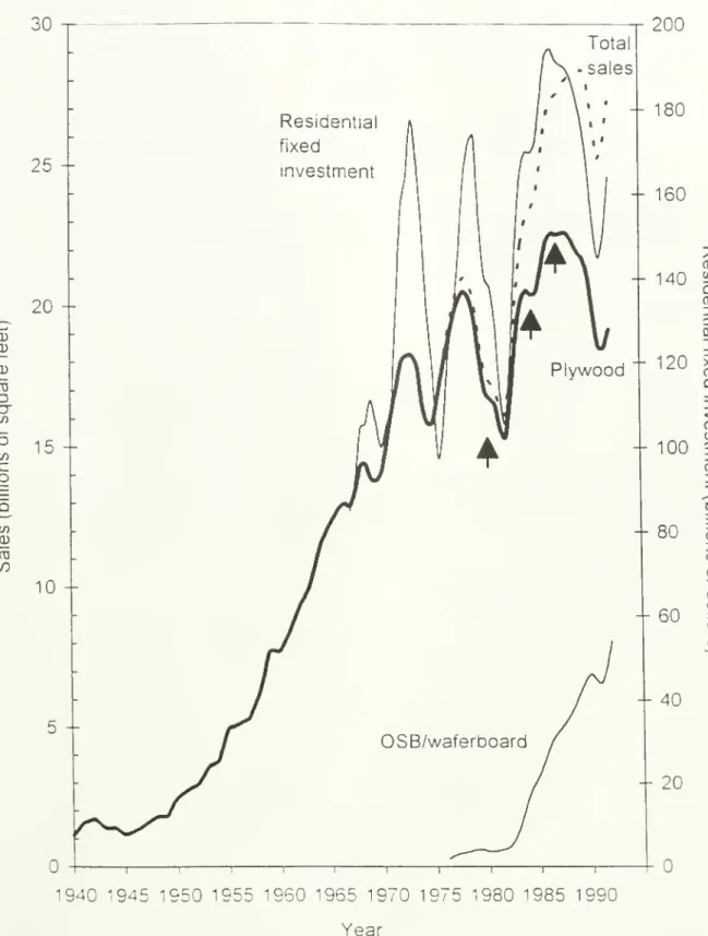
circumstances

Figure 1

shows

the sales o\~

phwood

and

OSB/waferboard

in the

US

Note

boss the

growth

curve of

plywood

grosss

smoothly

(with

minor

oscillations), but then breaks into

pronounced

oscillations in the

mature

phase, and hoss the

emergence

of

a ness

technology

(OSB

waferboard) coincides with the onset of oscillatory- behavior in the S-curve oi' the

mature technology

(plvwood

in this case) Since external factors such as those referred to in a

earlier in tins section

have

such an important influence

on

the rate ofdiffusion, is it reasonable

to assert that they, or other external factors, will also cause or influence the oscillations'1 If so.

this

would weaken

the

argument

that the oscillations are triggered by the

emergence

of

an

emerging technology

For

example. Girifalco points out that erratic behavior

from

the

smooth

S-curve can be attributed to changes in the business, political

and

social

environments

or to

the specific differing characteristics of the adopters [25] Davies has

shown

that the

growth

curve exhibits oscillators- behavior

due

to the fact that the industry (niche) is

expanding

or

contracting [17]

A

chaos

formulation has also

been proposed

by

Modis

and

Debecker.

and is

discussed later in this

paper

From

a mortality indicator viewpoint,

however,

the question that

arises is

whether

these oscillations are

brought

about by the

emergence

of a challenging

new

technology in

some way

or another Ifso. is this a necessary, sufficient

and unique

condition

for the oscillations

Obviously

if

one

can

show

that the oscillations are triggered

by

the

emergence

ofa

new

technology

{and only by the

emergence

of

a

new

technology), it will be an

extremely

powerful and

useful indicator with

profound

implications

on

the ability to identify

and track

emerging

technologies as well as

end-game

strategies for

mature

technologies

Alternatively, the

weaker

case

where

an

emerging technologv

also influences (but is not solely

responsible for) the oscillatory behavior in a

mature

technology's S-curve is also useful,

although less so and

more

complicated to apply operationally

Diffusion of

plywood and

OSB/waferboard

Montrey and

L'tterback investigated the diffusion of

plvwood

and

OSB

waferboard

in the light

frame construction industry [20.26] This case is discussed here as an illustrative

example

for

I-several reasons, viz it is a

good

example

of oscillatory behavior in a

mature

technology's

S-curve, it illustrates the interaction

between

two

technologies within thiscontext (as

opposed

to

just

one

technology

competing

against the

market)

and it has

drawn some

discussion in the

literature

After

World

War

II,

and

particularly since the 1950s,

plywood became

the

dominant

staictural

panel in the industry', having gradually displaced

lumber

as the preferred sheathing material for

floor, wall and

roof

construction

However,

since the late

1960s

several

developments

led to

the

appearance

of

new

unveneered

panels (notably

waferboard

and

OSB)

that started

challenging

plywood's

dominance

[20], viz

Technology

related

developments

There

were

process

advancements

for the

manufacture

of

chip or flake based panels

Raw

material

developments

The

prices

of

plywood were

increasing fast,

due

in part to the

depletion

of

suitable timber supplies for the

manufacture of

plywood

On

the other hand,

suitable

new

timber supplies for

unveneered

panels

were

being exploited at

lower

costs

Lately there has also

been

some

environmental pressures that tend to limit the

raw

material

supply of

plywood

Market

developments

The

remaining

raw

material supplv for

plvwood

had been

declining

in quality

Political

developments

There

had

been

some

changes

in building

codes

that

made

the

unveneered

panels

more

acceptable

The

new

unveneered

structural panels

were

mainly waferboard,

COM-PLY

and

OSB

first

marketed

in 1976. but had not

proven

to be a very successful product and has almost

disappeared as a serious competitor

OSB

has

been

commercially

produced

since 19S1 and has

been

very successful It has

proven

to be superior to

waferboard

and in

some

respects also to

plvwood

All three

of

the

plywood

substitutes are

marketed

as structural sheathing

commodities

Montrev

and Utterback

concluded

that

plywood

was. and

would

continue to be.

at a severe cost disadvantage with regard to the

newer

panels, and that there

was

no doubt

that

plywood

was

under

attack

from

the

newer

panels [20].

OSCILLATORY BEHAVIOR

OF

THE

S-CURVE

Consider

now

again Figure 1

which

shows

the sales

of

plywood

and

OSBwaferboard

in the

US

(as well as

combined

sales) in billions

of

square feet, calculated

on

a 3/8" basis

The

data

on

plywood

was

obtained

from

Montrey

and Utterback

for the period

1940-1975

[20]

From

1976

onwards

both the

plywood

and

OSB

data

were

obtained

from

[27]

Waferboard

and

OSB

have been

grouped

together as a category

of

unveneered

panels

competing

with

plywood

as in

Montrey

and Utterback's original

paper

[20]

The

sharp upturn in the curve for the

unveneered

panels in the earlv

1980s corresponds

with the introduction of

OSB

Note how

the

plywood

sales generally follows an S-curve

and

has a relatively uneventful life until

approximately

1970

when

the sales curve starts oscillating

The

fact that these oscillations

correspond

with the

emergence

of the

unveneered

panels

prompts

the question

whether

the

oscillations in

plywood's

S-curve are causally related to the

emergence of unveneered

panels,

i e

whether

the fluctuations indicate the presence ofa superior substitute

and

are triggered by

the resulting fluctuations in

demand

If so, it

would

lend credibility to the hypothesis that

attack

from

an

emerging

technology, and

hence

that oscillations can be interpreted as mortality

indicators

Montrey

and Utterback ascribe the oscillations in

plywood's

curve

throughout

the 1970s to

the '

erratic nature

of

the overall

wood

products

economy

during that

decade"

They

comment

that " the steep

drop

in the

mid-1970s

coincides with the nation's recession

during that period, during

which

housing construction

sank

to very

low

levels" In order to

test this statement,

we now

compare

residential fixed investment trends in the

US

with

plywood's

S-curve.

The

assumption

is that, since the light

frame

construction industry is a

major

contributor to the residential fixed investment and this industry is

one

of

plywood's

main markets

[28], an

examination

ofthe correlation

between

time series data for residential

fixed investment and

plywood

sales

would

be a

good

indicator to test the hypothesis that

oscillations in the curve for

plywood

are

coupled

to

macroeconomic

business cycles

Data

for

residential fixed investment

was

obtained

from

Gordon

[29] for the period

1950-1979,

and

from

Statistical Abstracts

o^

the

US

[30] for the period after that'

The

residential fixed

investment is also

shown

in Figure 1 (in constant

1982

dollars)

The

correlation

between

the

market swings

in the curve for residential fixed investment

and

the oscillations in the total sales

is remarkable

(Note

that

we

are looking specifically at the phases rather than the amplitudes,

since

we

are

comparing

sales in billions

of

square feet in the case

of

plywood

with billions of

dollars in the case of residential fixed investment ) Since

plywood

constitutes a

major

part of

the

market

share, it

would

be fair to

conclude

that sales of

plywood,

and

particularK the

oscillations in its S-curve. are indeed

coupled

to

macroeconomic

business cycles, specifically

residential fixed investment

One

should,

however,

be careful about the causality implied in

the residential fixed investment curve driven by the

plywood

sales"1

Ifthe latter is the case, it

may

be that the

plvwood

curve oscillates for reasons other than the residential fixed

investment

and

that the residential fixed investment only follows the

plywood

curve

A

more

plausible explanation is that the residential fixed investment in the

US

is

determined

by

macroeconomic

conditions and that it should be considered as a

"demand"

curve or driver in

this setting Surely decisions to build

new

housing is not

determined

bv the

amount

of timber

sold

—

rather the other

way

around

Timber

products are supplied inter alia to fulfill the

demand

for housing

and hence

the

plywood

curve followsthe residential fixed investment It is

also interesting to note

how

both the

plywood

and

OSB/waferboard

curves tend to track the

residential fixed investment in the latest years for

which

the data are given Recall that the

sharp upturn in the

OSB/waferboard

curve in the early eighties

was

caused

by the

emergence

o\~

OSB

as a technology It

would

seem,

however,

that as

OSB

becomes

an established

technology and gains significant

market

share, its fortunes are also linked to residential fixed

investment in a

more

pronounced

way

The

dips in the curves

around 1990

illustrate this point

It will be interesting to see if

OSB

continues to track the oscillatory behavior

of

the residential

fixed investment curve in years to

come, and

if the coupling

between

the

plywood

curve and

residential fixed investment decreases as

plywood

loses

market

share

The

arguments

in the previous paragraph leads

one

to

conclude

that oscillations in

plywood's

S-curve are primarily the result of fluctuations in the residential fixed investment pattern and

therefore are not triggered by the

emergence

of

OSB/waferboard

Hence

the oscillations

cannot be interpreted to be mortality indicators per se

The

question

does

arise,

however,

if

the

emergence

of the

new

technology contributes to

some

secondary or smaller perturbations

S-cun.es

of

plywood

and

OSB/wafcrboard

as well as the S-curve ofthe

combined

sales

Note

that there are three "hiccups"

superimposed

on

the general oscillatory pattern

of plvwood's

S-curve (indicated with small

arrows

in Figure 1)

At

the first hiccup, the

S-curve

of

plywood

tracks the

S-curve of

the total sales very closely

At

this point

OSB/waferboard

had

not really

made

anv

market

impact and the total sales for all practical

purposes

therefore represents the

sales

of plvwood. At

the

second

hiccup,

however,

the dip in

plywood's

S-curve is

much

more

severe than that

of

the total sales and furthermore there is

no

hiccup at that time in the

S-curve

of

OSB/waferboard

This could be interpreted to

mean

that the

plywood

sales lag total sales

for a while, but then catches

up

again It is

tempting

to speculate

on

the cause

of

this deviation

in the

plvwood

sales

One

hypothesis might

be

that the

demand

for structured panels

was

being taken

up by

the

unveneered

panels rather than by

plywood

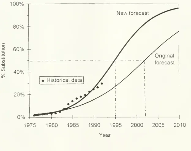
The

historical data in

Figure 2

shows

how

the

unveneered

panels gained

market

share at the

expense of plywood,

lending support this hypothesis- If this is the case,

why

does

plywood

then recover, as

indicated

by

the

plywood

curve that

resumes

growth

after the hiccup7

_A

_{possible explanation}

is that the

demand

for

unveneered

structured panels

was

greater than the capacity

and

that the

resulting slack

was

then taken

up

by

plywood

Table 1

shows

the

demand/capacity

ratios of

plywood

and

OSB

in the

US

for the period 1981

to

1989

[27] If

we now

focus

on

the period

1983-1987, which corresponds

with the period

where

the trends in

plywood

sales

seemed

to lag the trend in residential fixed investment cycle

as

shown

in Figure 1,

we

note that the industry

demand/capacity

ratio increased

from

SO

to

S7 (with a high of

OSS

in 19S6), re

SS°o

The

demand/capacitv

ratio for

plywood

increased

from

S2 to 0.8-4 (with a high

of

87

in 1986), i.e 2

4%

However,

the

demand

capacity ratio for

OSB

increased

from

58 to

90

(with a high of 93 in 1986). i e

55°o

There

is thus evidence of a

much

steeper increase in the

demand/supply

ratio for

OSB

than for

plvwood

This

mav

indeed indicate that

OSB

supplv

was

harder

pushed

to

meet

demand

and hence

unfulfilled orders might

have been

filled by

plywood

Note

that even

though

capacity

was

still larger than

demand,

there might have

been

regional factors, for example, that

caused short

term

shortages in

OSB

This explanation of interaction

between plvwood

and

OSB/waferboard

can account for the hiccup in the

plywood

curve

around

1985, and so lend

support to the larger hypothesis that an attacking

emerging

technology can contribute to the

perturbations in a

mature

technology's

S-curve

In order to identifv such a

phenomenon,

one

would

thus typically subtract the sales curve

of

the contributing technology

from

the total sales

curve

and

isolate irregularities

The

third hiccup

seems

to exhibit a similar behavior

where

both

the total sales

and

that

of

OSB/waferboard

is growing, but the sales

of

plwvood

is dipping

Just as

one

tree

does

not

make

a forest,

one

or

two

hiccups in an S-curve

do

not constitute an

oscillatory pattern

However,

the

arguments

above

support the general conclusion that an

oscillatory pattern in the S-curve are not necessarily triggered bv the attack

from

an

emerging

technology

What

does

seem

plausible,

however,

is that an

emerging technology

can. together

with other factors, give rise to perturbations in the S-curve (but not necessarilv to

oscillations)

Given

the

arguments advanced

in the previous paragraph, this statement should

immediately be qualified bv saving that such perturbations should be carefullv analyzed within

the context of other influences (such as

macroeconomic

business cvcles) and that the

mere

existence

of

oscillations or perturbations is not

enough

to qualify' as a inortalitv indicator

One

of the difficulties, of course, is to distinguish

between

such indicators

and

regular statistical

fluctuations

As

the data

on

the residential fixed investment shows, the oscillations can be

effects o\~ the

emerging

technology Interpreting the signal thus entails

more

than just

observing an oscillators' pattern or perturbations

As

this

example shows,

external influences

such as the general

economic

climate and business cycles can play a significant role

Taking

into

account

measurement

errors

and

other sources

of

fluctuations

and

oscillations mentioned,

together with effects caused by business cycles, it is evident that a certain

amount

of signal

processing will

have

to be

done on

an S-curve to extract potential signals

from emerging

technologies

FORECASTING THE

SUBSTITUTION

PROCESS

Montrey

forecasted the substitution

of

OSB/waferboard

for

plywood

in

1982

[26] Treating

waferboard

and

OSB

as

one

product category

and

using a Fisher-Pry

model

[31], he

formulated the forecast in the

form

/(0

=

-[l

+ tanha(/-/

)] (1)

where

f(t)

=

fraction of takeover

of

OSB/waferboard

in yeart

a

=

half the initial exponential takeover rate

t

(l

=

year in

which

the substitution is

50%

completed

The

constants

were found

to be

a=0

071 1

and

t

=2002.

i.e the forecast indicated that half the

US

structural panel

market

would

be

made

up of unveneered

panels

(waferboard and

OSB)

by

the year

2002

In their 19 Q paper.

Montrey

and Utterback refer to the

19S2

forecast, and

specificallv to the fact that a

14S°o

substitution

was

predicted for

1985

whilst the true

substitution

was

in fact

15%

[201

(However,

based

on

the constants given in their paper, it

would

seem

that the

model

given in their

1990

paper actually predicts a S

16%

substitution

rather than a 14

8%

substitution in 1985

Hence

the rate substitution

was

even

brisker than

they predicted).

Having had

the benefit

of

several

more

years ofhistorical data, the temptation

of updating the forecast again

was

too great to resist (and in retrospect probably against the

present authors' better

judgment)

Subsequently the substitution data

of

OSB/waferboard

for

plywood

for the period

1976

to

1992

was

applied in a Fisher-Prv

model

similar to the original

one

described bv

Montrey

and Utterback.

The

parameters for the

new

forecast

were

determined with the software

accompanying

Porter el al.'s

book

[4]

Based

on

the

new

data.

the coefficients for the

new

forecast

were

found

to be

a=0.10S7

and

t„

=1995

As

in the

original forecast, it

was assumed

here that

plywood

and

OSB/waferboard

address the

same

market segments

and that they

account

for the total

market

between them

This

assumption

is

a

rough

approximation, since

Montrey

and

Utterback state that there are mutually exclusive

market

segments

for both

plywood

and

OSB

[20]

The new

forecast is

shown

in Figure 2 together with the historical data as well as the original

forecast

According

to the

new

forecast, the substitution will be

50%

completed

in 1995

The

fact that this forecast predicts a stronger current

showing

for

OSB

than is evidenced bv the

current historical trend is slightly worrying.

However,

there is strong evidence that

OSB

will

continue to

grow

at the

expense

of plywood.

As

of

September

1994

there

were

indications

that at least 15

new

OSB

plants

were

likely to be build in

North

America

before the turn ofthe

centuiA [32] At the

same

time there is also evidence ofa falling

plywood

production This is

in

pan

due

to the lack of raw material, environmental pressures

and governmental

resource

this

purpose

[33]

The

statement that

New

oriented strand

board

mills,

meanwhile,

have

filled the void left as

plywood

mills shut

down

because

they couldn't get big logs to peel

As

even

more

oriented strand

board

capacity is added, it

may

elbow

aside older

plvwood

mills

with uncertain

and

expensive log supplies" [34], is typical of opinions expressed in the

media

circa late

1994

The

issue is

whether

capacity to

manufacture

OSB

can be

made

available as

fast as

plywood

capacity falls

away

[35]

As

a defensive strategy,

one

can expect

plywood

manufacturers to target niche

markets

that are not addressed

by

OSB

A

chaos formulation

We

now

turn our attention to alternative explanations for the oscillatory behavior This part is

introduced by a discussion

of

a previously

proposed chaos

formulation,

and

is then followed

by the presentation of a modified Lotka-Volterra

model which

illustrates

how

the symbiotic

interaction of

two

technologies can give rise to oscillatory behavior in the

mature

phase of an

S-curve

Referring to the oscillatory behavior in the

mature

phase

of

some

technologies' S-curves,

Modis

comments

that "

_These

_deviations

_{have been}

_{explained in terms}

_of

_{states of chaos,}

which

are

encountered

when

the logistic function is put in discrete form,

which

becomes

essential in order to analyze data via

computer

programs which

employ

iterative techniques,

but it can also be justified theoretically

because

populations are discrete quantities after all"

[24] In another article

Modis

and

Debecker

make

the

comment

that "

The

annual rate of a

population

growth

into a

new

niche had often

been

seen to follow a logistic pattern that brakes

into fluctuations ol~

random

character and sizable amplitude just before reaching the ceiling"

[22]

Thev

then

proceed

to explain the oscillatory behavior of the

growth

curves with

chaos

,. c,.

theory

Modis

and

Debecker's

paper suggests a justification for an investigation into the

seemingly chaotic nature

of

the oscillations in the

mature

phase

of

S-curves

In addition to

Modis

and Debecker's

contributions, several other articles

have been

published

over the last couple

of

years to

show

the relevance ofchaotic behavior and the associated use

of fractals to

growth

models

of technologies and technological forecasting (see for

example

Gordon

and

Greenspan

[36,37],

Bhargava

el al. [38],

Gordon

[39,40] and

Modis

[23.41])

The

conclusion that

Bhargava

el al.

come

to is telling of the sentiment of

many

ofthe papers,

viz "... the

importance of

the logistic equation in describing

economic

and

social behavior is

undeniable

However,

one must

be prepared for the greater richness

of

the behavior of the

solutions, particularly for large values of the nonlineantv

parameter

X" [3S]

The

logistic

equation that is referred to is the discrete difference equation

form of

the differential equation

for

which

(1) is the solution, and

which

leads to chaotic

and

oscillatory behavior

when

X

is

large (X being a

parameter analogous

to

a

in (1))

According

to the narrative in

Modis

and

Debecker's

article [22], they

happened

upon

the

chaotic behavior whilst searching for

ways

in

which

to speed

up

algorithms to generate

S-curves

By

discretizing the calculation, they not onlv

succeeded

in generating the S-curves, but

also fluctuations in both the initial and

mature

phases of the curve

Recognizing

that the

fluctuations

were

akin to the oscillations that are often

observed

on

growth

curves, they

investigated the appropriateness

of

a chaos explanation for the

phenomenon

Thev

proceeded

to investigate the effect by

changing

the nature

of

parameters in the discrete representation of

the S-curve Their simulations yielded systems with seemingly chaotic behavior, and

hence

their claim that

chaos

theory can account for the

S-shaped growth

curve, oscillations in the

mature

phase of S-curves. as well as similar fluctuations often

observed

in the early

growth

phases ofa technology

They

also suggest that chaotic behavior can exist in the transitionary

period

when

one

S-curve is replaced

by

another, i.e.

when

the

mature phase of one growth

curve is blended into the early phase

of

the next curve

The

annual production

on bituminous

coal in the

US

is held as an

example

Modis

and

Debecker's

statements that ".

_One

_{could reasonably expect} that an

upcoming

growth

phase in a

new

market

niche will be heralded by precursors and,

once

installed, will

proceed

at an accelerated

rhythm

in the beginning",

and

"

_A

_{well-established}

_S-curve

_will

point to the time

when

chaotic oscillations should be expected; it is

when

the ceiling is being

approached

In contrast, an entrenched

chaos

will reveal nothing about

when

the next

growth

phase will start" [22] deserve

some

comment

The

notion

of

precursors that indicate a

new

growth

phase is

noteworthy and

lends support to the hypothesis that oscillatory behavior (or

perturbations) in the

mature

phase

of

technology's

growth

may

indicate the rise of an

emerging

technology

Drawing upon

the inherent

determinism

in chaotic systems,

Modis

and

Debecker

seem

to imply,

however,

that there is a certain inevitability in the onset

of

the

chaotic oscillations

Gordon

alludes to the

same

notion

when

he savs

of

chaotic oscillations

generated by a simulation

of

sales as a function oftime, "

An

analyst

would

understandably,

wonder

about the causes for the

market swings

What

caused

them

9 _{In fact,}

_no

_{externalities}

were

responsible, all

of

the

complex

behavior ofthis curve results

from

within the

system

...

To

search for externalities responsible for the

market

performance

would

be

misplaced effort,

for in this example, all

of

the chaotic behavior

comes

from

internal sources" [40]

Modis

refers

to

Montrey

and Utterback's explanations for the fluctuations in the

growth

curve of

plywood

b\ stating that "

_From

₁₉₇₀

_onward

a pattern of significant (plus or

minus 20

percent)

instabilitN appeared,

which

Montrey

and Utterback

tried to explain

one

by

one

in terms of

socioeconomic arguments

Given

a pattern

one

can always

correlate other

phenomena

to it

This type ofpattern,

however,

could

have been

predicted a

pnon

by chaos formulations" [23]

The

arguments

presented in the previous section

seem

to indicate,

however,

that the residential

fixed investment did play a

dominant

role in determining

the oscillatory behavior in

plywood's

S-curve

The

chaos-based

model

that

was

referred to in this section describes a

technology

which

competes agamst

the market, i.e. the formulation

does

not explicitly

account for the effects of

one

or

more

technologies Often

one

finds,

however,

that

two

or

more

technologies are

competing

or are interacting with

one

another in a given

market segment

In the next section a

mathematical

model which

involves

two

interacting technologies and that can also

lead to

oscillator, behavior, is described This

model

is applicable

to the general case of

two

interacting technologies and is not restricted to the interaction of

emerging

and

mature

technologies It should be stressed that the

model

is presented as

a conceptual one, very

much

in the

same

vein as the

chaos

formulation

of

Modis

and Debecker

[22], rather as

one

that has

withstood the test of time

Modeling

the oscillatory

behavior with modified Lotka-Volterra

equations

The

differential equation.s) describing the diffusion of a technology

must

be

based

on

the

underlying

mechanisms

involved In order to

model

the

diffusion characteristics of a

technology, it is therefore necessary that the extent of the

resources available be taken into

account Finite resources are often

embodied

in a

market

niche

offinite size

A

single equation

cannot,

however, descnbe

the

growth

and competition of

it does not account for their respective effects

on

one

another It can at best

model

the

diffusion of

one

technology into a

market

[42]

To

model

the competition of

two

technologies,

one

would

need to set up a differential equation for each

of

the technologies based

on

the

underlying drivers and inhibitors for that technology, together with coupling coefficients that

reflect the technologies" effect

on one

another's

growth

rate In order to address the

problem

at hand, it is necessary to

model

both the technologies explicitly, each with its

own

equation

They

must

then be

coupled

with coupling coefficients to

account

for the interaction

between

them

A

system

of differential equations rather than a single equation is therefore required

Such

a

system

that is applicable to this

problem

has

been

formulated

some

time

ago

bv the

ecologists

Lotka

and Volterra. but until very recently

was

not widely applied to the diffusion

of technology

The

system of equations that they

developed

has

become known

as the

Lotka-Volterra equations

Several authors

have

shown

or

commented

on

the fact that the

Lotka-Volterra

equations can

be successfully applied to

model

technological diffusion,

among

them Bhargava

[43], Farrell

[44], Marchetti [21,45],

Modis

[23],

Nakicenovic

([46] as

quoted by

Marchetti [45])

and

Porter el al. [4] Marchetti

comments

that '

I

am

fairly

convinced

that the equations Volterra

developed

for ecological

systems

are vers'

good

descriptors

of

human

affairs In a

nutshell, I

suppose

that the social system can be

reduced

to structures that

compete

in a

Darwinian way,

their flow and ebb being described bv the Volterra equations, the simplest

solution of

which

is a logistic" [21 ]

Even

though

the Lotka-Volterra equations

may

be suitable to

model

technological diffusion

and substitution, the question arises

however,

as to the appropriateness

of modeling

the

oscillatory behavior in the

mature

phase of the S-curve, with these equations

There

are

several references in the literature that suggest that the Lotka-Volterra equations

may

indeed

lead to a

modeling

solution for the oscillatory behavior that

we

are

concerned

with here

Porter el a!., for example, state that " Oscillatory

models

are a final class of

models

accommodated

by the Lotka-Volterra equations Periodic behaviors are

commonly

found

in

natural populations and they can be successfully

modeled

using the Lotka-Volterra equations

Oscillators' behaviors

have been

observed in

consumption and

mining patterns in the 'united

States and in car

and

transportation systems in

Europe

These growths

often

show

a

logistic start followed

by

an overshoot and then oscillation

around

a

supposed

limit

The

more complex

population

models

such as Lotka-Volterra, can represent such behaviors if the

forecaster has correctly surmised their

form..."

[4]

The

above

reference to a logistic equation

that overshoots and then oscillates

around

a limit is strongly indicative

of

the type of

oscillations that

we

are interested in, i.e those that are

sometimes observed

in the

mature

phase

of

a technology Recall also Marchetti's

comment

quoted

earlier to the effect that

S-curves can

become

oscillatory

when

approaching

saturation

and

that this is a possible solution

of

Lotka-Volterra equations

Consider

now

two

technologies

which

are interacting in a symbiotic

way

Symbiosis

is an

ecological

term and

refers to the association of

two

different

organisms

Using attached to each

other or

one

within the other to their

mutual advantage

The

term

is related to the concepts of

mutualism and commensualism,

but for the

purpose

ofthis discussion, it is

meant

to imply the

interaction

among

two

technologies such that each has a positive influence

on

the other's

growth

rate

A

system ofnonlinear differential equations

(which

is

based on

Lotka-Volterra

ciN _, dt

—

= a

_n

N-b

_n

N-

+c

_nm

NM

(2)

dKl

,

—

=

a

_m

A

1

-

b,„

A

I~

+

c

_im

A4N

(₃ )

where

N(t)

and

Al(() represent the "populations"

of

the

two

technologies (such as sales, for

example)

and all coefficients are positive This set of equations differs

from

traditional

Lotka-Volterra equations in the sense that both ^-coefficients are positive,

and

furthermore has

been

modified to depict symbiosis

by

having positive signs for

both

the coefficients that regulate the

interaction

among

the

two

technologies (c

_nm

and

c

_mn

).

A

generic phase

diagram

for this

formulation is

shown

in Figure 3.

The

equilibrium lines

on

the associated

phase

diagram

that

indicate

where

dN

di=0

and dhl

dt= Q are respectively given

by

N

=

^L

+ ^SL

M

₍₄₎

b„ o„

M

h"< _KA "'"

c..,„ c..

inn

The

axes of the

phase diagram

are also equilibrium lines, i e

dM/dt=0

on

the yV-axis

where

A/-0

and

dN.dt=0 on

the A/-axis

where N=0. The

equilibrium point

(N*,M*)

represents the

position

where

dN

dt

=

and

dM/dt=0

simultaneously (i e the intersection

between

these

two

lines) and is normally a stable point, in the sense that

once

it has

been

reached, the trajectory

will terminate there

The

arrows

in the four subregions

of

the

phase

diagram

indicate the

directional derivatives in those regions

Note

that time is a

parameter

for a trajectory

on

the

phase

diagram

Pielou's iterative solution for the set of equations [47] are modified to account for the

symbiotic interaction, yieldingthe solution

where

and

where

N(t +

l) ;

_{v N(t)}

fc

)

\-P

n

N(,)-\^\P

n

MU

(6) ?

=

ea" (7)

P„

b n(e a »

_-1)

(8)

M(l

+

1)

X,„M{t)

\

+

p

m

M{t)-C

-f

L \ (9)

An "

L' 10) p, b,„(ea

»<-\)

(11)

In order to illustratethe

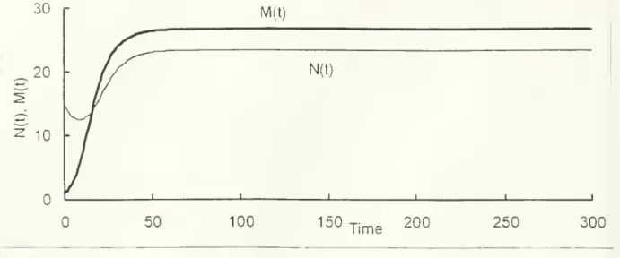
dynamics

ofthis formulation, consider

now

the

system

\'{D=

.Y(0.1-0.01.V-c„„

(A/)

( 1

.\/m

=

A/(0

15-001.\/-c„„,.Y)

(13)

with c„„,=0.005

and

c

_mn

=0.005

Let the initial _{conditions be Af(0)=\}

_and

_N(0)=\5

It should

be stressed that the

numeric

values

of

the coefficients as well as the initial values are not

intended to relate to any real situation

—

the coefficients

a

and b in this

example

were

randomly chosen

with c adjusted to illustrate the

dynamics

conceptually

The

resultinu time

domain

plot

and

associated phase

diagram

are

shown

in Figures 4

and

5

Note

how

the

trajectory

on

the phase

diagram approaches and

terminates

on

the equilibrium point

Coming

back

to the oscillatory behavior in the

mature phase

of an S-curve,

we

note that an

interesting

phenomenon

occurs

when

c

_mn

c

_mn

approaches

b„b

_m

Consider

again the phase

diagram

in Figure 3

As

expected, a trajectory that initiates in subregion 1

approaches

the

equilibrium point

However,

rather than terminate at the equilibrium point (as in Figure 5), the

trajectory

seems

to

overshoot

and then breaks into an oscillatory pattern

A

cursory inspection

ofthe oscillators' pattern in the time

domain

reminds

one of

a chaos-like state Figures 6

and

7

show

the time

domain

plot and phase

diagram

when

c

_m

„=0.005

and c

nwi

=0.0157,

yielding

values

of

b„b„ =0.000]

and c„„,t„„,=0

000079

(whereas

in the previous case

c_iwic_'>nn

=

_Q

000025)

Both

_{technologies live fairly uneventful lives in the}

time

domain,

following

regular

growth

along S-curves until

approximately

/

= 240

when

they

both

break _into

chaos-like oscillatory patterns

By

examining

the time

domain

plot in Figure 6,

one might

wonder

what

gives rise to the

sudden

burst

of

oscillations in the

mature

phase after the

two

technologies coexisted for a long time during

which both

followed

normal

logistic

growth

It

turns out that there is _{nothing mystical about the time}

_when

_the

oscillations start

An

examination

of

the associated phase

diagram

in Figure 7 reveals that the time

when

the

oscillations start corresponds with the time

when

the trajectory in the phase

diagram

reaches

the equilibrium point Ifthe coefficients are

known,

the phase

diagram

can be constaicted and

subsequently the time

when

the oscillations will

commence

can be predicted

The

chaotic oscillations

observed

here are a far cry

from

those

shown

in Figure 1

Note

that

the

two

technologies simulated in Figure 6 break into oscillations simultaneously

—

something

that

plywood

and

OSB/waferboard

in Figure 1

do

not

do

Keep

in mind,

however,

that the

system

shown

here is purely to illustrate the concept, and that the possibility that the

plywood/OSB/waferboard

case cannot be

modeled

with this

model

should not be dismissed

out

of hand

without further investigation

of

the behavioral characteristics

of

the

model

It

should also be kept in

mind

that the simulated results presented here

were

generated with a

difference equation

and

the time increments in the

model

hence plays an important role in the

behavior, particularly

when

a chaotic situation occurs.

Note

that the

model

also

sometimes

yieldsnegative values for

N

and

A-/,

something

that cannot occur if

N

and

M

represent the real

sales of the technologies for example,

where

we

assume

M,N>0.

Nevertheless, the results

obtained here indicate that, in principle,

one

can expect oscillatory behavior in the

mature

phase of S-curves

under

certain

circumstances

when

two

technologies

have

a symbiotic

interaction

From

the nature

of

equation (1)

we

know

that in the

absence

of

another

technology, oscillatory behavior

does

not

occur

and hence

we

can infer that (within the realms

ofthe model), the chaos-like oscillations in the

mature

phase ofthe S-curve can also be caused

bv symbiotic interaction

among

multiple technologies, in

which

case the onset of chaos

depends

very strongly

on

the ratios of the coefficients in the underlying Lotka-Yolterra

equations

Note

that the system

modeled above changed

its behavior

from

stable to oscillatory

when

the

ratios of the coefficients

changed

(i e the

change

depicted in Figures 4

and

5 versus that in

Figures 6 and 7) In general,

one

can

assume

that the coefficients will be time

dependent

rather

than constant, and furthermore that external forces can and will influence their values

dvnamically with time It is then entirely conceivable that a chaotic solution

may

result if the

values

of

the coefficients

change

relative to

one

anotherto support such a solution This brings

us

back

to the issue

of

the

pre-determinedness of

the chaotic nature that has

been

discussed in

the literature

The

issue boils

down

to the question

whether

the

growth curve

that a particular

technology

exhibits is genetically

encoded

into the technology (similar to the

growth of

some

animate or organic objects, for

example)

If

one

takes the

view

that technological diffusion and

substitution are social rather than natural

phenomena,

there is an

argument

to be

made

that

there is

no predetermined

inevitability in the

growth

of technology

The

diffusion pattern and

particularly the rate

of

diffusion, are

determined

by various external factors, although

we

certainly

acknowledge

that the inherent characteristics of the innovation or

technology

can

influence these factors

We

must

also not exclude the possibility that,

from

a

modeling

viewpoint, the

growth

of

a particular

technology

may

be described

by

different

models

along

its

growth

path, as suggested

by Tingyan

[48], for

example

It is quite feasible that the

growth

may

be described by the general Lotka-Volterra equations as suggested

by Bhargava,

where

the coefficients of the equations

change

with time as they are acted

upon

by external

forces [43]

Depending

on

the relationship

and

ratios

between

the coefficients, the

svstem

may

then exhibit

smooth

growth, oscillatory or

even

chaotic behavior in various phases

of

the

growth

cycle

These

will be dictated by the ratios of the coefficients at

any

given

moment

as

thev. in turn, are influenced bv external forces

Even

thouuh

some

technological

urowth

patterns

may

exhibit chaotic oscillations, the question that should be

asked

is.

"What

drove

the

system to chaos "

[39]

Conclusions

The

paper started

by

discussing the notion

of

mortality indicators that signal the

demise

of

mature

technologies

The

question

was

posed whether

the oscillations that

have been observed

in the

mature

phase of

some

technologies' S-curves are indications that such technologies are

being attacked

by emerging

technologies, i e

whether

the oscillations are mortality indicators

The

case of the substitution

of

plywood

by

OSB/waferboard

was

investigated, and it

was

shown

that the oscillations in

plywood's

S-curve track the phases

of

the residential fixed

investment in the

US

Hence

it is

concluded

that the residential fixed investment pattern is

therefore primarily responsible for the oscillations and that the oscillations are not mortality

indicators

The

rise

of

OSB/waferboard

does,

however,

seem

to contribute to perturbations in

the

mature

technology's S-curve

(plywood

in this case)

A

further conclusion can thus be

made

that the

emergence

of a

new

technology can

have

a contributory influence

on

perturbations in a

mature

technology's S-curve, although the oscillations can be

dominated

by

other effects such as

macroeconomic

business cycles

Given

the fact that accurate and reliable

mortality indicators can

have

profound

managerial implications

and

that the surface has only

been

scratched in this paper with regard to death knells of

mature

technologies, further pursuit

of the notion

of

mortality indicators is certainly to be

recommended

One

avenue

of research

may

be the application

of

signal processing techniques to "extract" potential signals that are

caused b\

emeruinu

technologies