Design and evaluation of freeway incident detection algorithms

Design and Evaluation of Freeway Incident Detection

Algorithms

by

Sreeram Thirukkonda

Indian Institute of Technology, Madras, India (1997)

Submitted to the Department of Civil and Environmental Engineering

in partial fulfillment of the requirements for the degree of

Master of Science in Transportation

at the OF TECHNO

MASSACHUSETTS INSTITUTE OF TECHNOLOG

June 1999

@

Massachusetts Institute of Technology 1999. All rights r

e

Author..

...

Department of Civil and Environmental Engineering

/

May

21,

1999

C ertified by ...

-...

Moshe E. Ben-Akiva

Edmund K.Turner Professor of Civil and Environmental Engg

Certified by ...

...---Mithilesh Jha

Research As ociate, Center for Transportation Studies

II001Ii

1

'1Thesis

Supervisor

Accepted by...

Andrew J.Whittle

Chairman, Department Committee on Graduate Students

Design and Evaluation of Freeway Incident Detection Algorithms

by

Sreeram Thirukkonda

Indian Institute of Technology, Madras, India (1997)

Submitted to the Department of Civil and Environmental Engineering on May 21, 1999, in partial fulfillment of the

requirements for the degree of Master of Science in Transportation

Abstract

A reliable, automatic freeway incident detection system is an important component of an

effec-tive incident management system. A traffic surveillance system equipped with loop detectors and speed traps can detect an incident by analyzing traffic measurements. Incident detection algo-rithms(IDAs) are the tools used to analyze these measurements. This work studies the limitations of current IDA evaluation methods and introduces some new approaches to incident detection. Case studies on 1-93 North and 1-90 West highlight the limitations of existing evaluation approaches. The algorithms perform optimally in a small subset of scenarios. The results of the case study indicate that it is imperative to evaluate IDAs over a broad range of scenarios to fully understand their applicability and transferability. The results also show that it may be advantageous to com-bine algorithms which have complementary characteristics under different scenarios to optimize overall performance. The feasibility of this approach has been demonstrated by combining a sim-ple algorithm based on observing speed drops at a sensor with the McMaster algorithm.

A new approach to incident detection based on discrete choice models has been introduced and

evaluated. This approach uses logit models based on traffic flow variables to identify congestion caused by incident. The performance of these algorithms has been studied over different scenarios. Using already existing methods, the logit models can be estimated with both simulation and real data to make the parameters both robust (simulation data from different scenarios) and easily trans-ferable to the field (real data). A case study based on real incident data from 1-880 near Hayward, California illustrates the advantage of this approach. A choice model based framework to combine different algorithms has also been presented. This framework uses the decisions of different algo-rithms to identify incidents. A model based on this framework has been estimated and evaluated over a set of scenarios.

Thesis Supervisor: Moshe E. Ben-Akiva

Title: Edmund K.Turner Professor of Civil and Environmental Engineering Thesis Supervisor: Mithilesh Jha

Acknowledgments

I would like to thank my supervisors Professor Moshe Ben-Akiva and Mithilesh Jha for their

guid-ance, support and encouragement at all stages of research. I would like to think Qi, Kazi and other

ITS staff for their guidance and support in implementation. I would like to thank Alan for all the

technical discussions and suggestions.

I would like to thank Bechtel,PB for funding this research. I would like to thank Cynthia Stewart

and her staff for their support and cooperation.

I would like to thank my lab mates and ex-lab mates: Masroor, Dave, Sridevi, Mark for his

in-teresting opinions of life, Mathew, Atul for all the coursework discussions, Bruno, Tomer, Jillian and Joan & Scott for the choice model discussions. I would also like to thank my friends at MIT for those lighter moments of life -Ninja, Harish, Megs, GV, and OP.

Contents

1 Introduction

1.1 Research Motivation . . . . 1.2 Literature Review . . . . 1.2.1 Impact of System Characteristics on Incident Detection . 1.2.2 Impact of Algorithmic Parameters on Incident Detection

1.3 Thesis Contribution . . . . 1.4 Thesis Outline . . . .

2 Calibration of the McMaster and APID algorithms

2.1 Description of the system . . . . 2.2 The McMaster Algorithm . . . .

2.3 The APID Algorithm . . . .

3 Evaluation of the McMaster and APID algorithms

3.1 Refinements to the McMaster algorithm . . . .

3.2 Refinements to the APID algorithm . . . .

3.3 Evaluation Results . . . . 3.3.1 Evaluation on 1-90 West . . . . 3.3.2 Evaluation on 1-93 North . . . . 12 . . . . 13 . . . . 14 . . . . 17 . . . . 18 . . . . 20 . . . . 21 22 . . . . 22 . . . . 23 . . . . 26 30 . . . .. 30 . . . 32

4 A Heuristic algorithm for dense loop detector spacing

4.1 Introduction . . . - - - . .. . - . . . 4.2 The Proposed Method . . . .. - . .

32 32 35 44 44 44 4

The Framework . . . . Experiments on 1-93 North . . . . Summary and Findings . . . .

5 Discrete choice models for incident detection algorithms

5.1 Introduction . . . . 5.2 Model Specification and Estimation . . . . 5.2.1 Binary Logit model to identify congestion . . . .

5.2.2 Binary Logit model to identify incidents . . . .

5.2.3 Binary Logit model to distinguish between incident ar 5.2.4 Multinomial Logit model . . ... . . . .

5.2.5 Nested Logit model . . . .

5.3 Model Evaluation using MITSIM . . . .

5.3.1 Limitations of Simulation . . . .

5.3.2 Summary of Results . . . .. 5.4 Comparison of performance of different algorithms . . . . .

5.5 Combined Estimation using real and simulated data . . . . .

5.5.1 Introduction . . . . 5.5.2 Real data . . . .. 5.5.3 Simulation data . . . . 5.5.4 5.5.5 5.5.6

Model structure for Combined Estimation -NLRPSP Results of Combined Estimation . . . . Using the RP-SP for prediction . . . .

6 Combining different algorithms for improved performance 6.1 Combining the SPDDRP and McMaster algorithms . . . . .

6.1.1 Introduction . . . .

6.1.2 M ethodology . . . .

6.1.3 Framework . . . .. . .. 6.1.4 Evaluation of the combined algorithm . . . .

49 . . - - . . - .- - 49 . . . . . 50 . . . . 51 . . . . 53 d recurrent congestion 56 . . . . 59 . . . . 62 . . . . 65 . . . . - - . 66 . . . . - . . . . 67 . . . . 67 . . . . 68 . . . . 68 . - - . - - - - . . . . 69 . . . . 70 . . . 72 . . . - - . 74 . . . 74 77 . . . . 77 - - - 77 . . . 78 . - - - . . . 78 . . . . 80 4.3 4.4 4.5 45 47 48 n

6.1.5 Findings and Summary . . . .

6.2 Using a LOGIT model to combine algorithms . . . .

6.2.1 Introduction . . . .

6.2.2 Testing of the models . . . .

6.2.3 D iscussion . . . .

7 Summary, Conclusions and Future directions

7.1 Summary and Conclusions . . . .

7.1.1 Evaluation of the McMaster and APID algorithms

7.1.2 Detecting incidents based on speed drop: SPDDRP

7.1.3 Discrete choice model based Incident Detection . .

7.1.4 Combining algorithms . . . . 7.2 Future Research . . . . 80 83 83 88 90 91 . . . . 9 1 . . . 9 1 . . . . 9 2 . . . 9 3 . . . 9 3 . . . 9 4 96 A Results of Calibration B 1880 Geometric Layout C 1880 Layout of Sensors

D Sample plots from real data

102

103 104

105 E Geometric Layout of the CA/T network

List of Figures

2-1 1-93 North Bound . . . .

2-2 Fundamental Diagram of Traffic Flow . . . .

2-3 Flow Occupancy plot for a sensor . . . . 2-4 Sample plot of McMaster threshold curve with the t97.5% confidence curves

2-5 OCCDF plots for incident and non-incident cases from simulation . . . . 2-6 OCCRDF plots for incident and non-incident cases from simulation . . . . .

3-1 Plot of M OEs . . . . . . - - - -. . . . .

3-2 Plot of M OEs . . . .. . . .. . . . . 3-3 Incident Locations . . . .. . . . . .

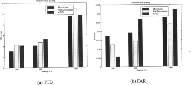
3-4 TTD and FAR vs spacing at 100% flowrate with pers=3 at location 2 . . . . .

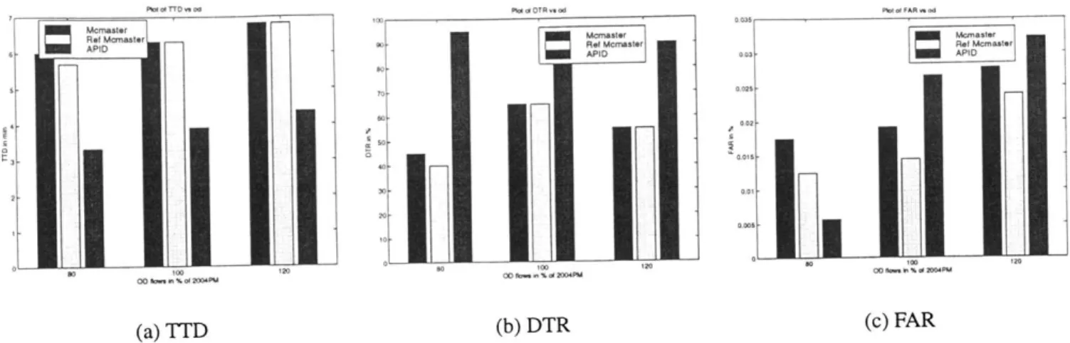
3-5 TTD,DTR and FAR vs Flow rate at 600ft spacing with pers=3 at location 1 3-6 OCCDF and OCCRDF for 2 stations on either side of an on-ramp . . . . 3-7 TTD,DTR and FAR vs Location at 200ft spacing,pers=3,od=100% . . . .

4-1 Speed Drop and Occupancy Rise at station upstream of incident . 4-2 Framework to declare incidents . . . .

Predicted probabilities for location 1 Predicted probabilities for location 2 Comparison of SPDDF with SPDRDF Predicted probabilities for location 1 Predicted probabilities for location 2 Predicted probabilities for location 1

. . . 45 . . . . 46 . . . . 5 2 . . . 5 3 . . . 54 . . . . 5 5 . . . . 56 . . . . 5 8 23 23 26 27 28 29 35 35 36 40 41 41 43 5-1 5-2 5-3 5-4 5-5 5-6

5-7 5-8 5-9 5-10 5-11 5-12 5-13 5-14 5-15 6-1 6-2 6-3 6-4

Predicted probabilities for location 2 . . . . Occupancy Difference at Location 2 . . . . Predicted probabilities for location 1 . . . . Predicted probabilities for location 2 . . . . Nested logit model structure . . . . Predicted probabilities for location 1 . . . . Predicted probabilities for location 2 . . . . Nested logit model structure for RP-SP Combination Predicted probabilities . . . .

Summary of Results . . . . Combination of SPDDRP and MCM . . . .

FAS vs TTD at 200ft spacing . . . .

DTR vs FAS at 200ft spacing . . . . B-I Layout of 1880 from www.mapquest.com

C-I Layout of 1880 from www.mapquest.com

D- 1 flow/occ/spd plots . . . . . . . . 5 8 . . . . 60 . . . . 6 1 . . . . 6 1 . . . . 6 3 . . . . 64 . . . . 6 5 . . . 7 3 . . . . 7 6 . . . 7 8 . . . 7 9 . . . . 8 1 . . . . 8 2 . . . 102 . . . . 1 0 3 . . . . 104

E-I The CAT network . . . . 105

OCCmax squared for different degrees . . . .

R-square and Adjusted R-squared for different degrees . . . . Typical parameter values for a station for the McMaster algorithm

Measures used by the APID algorithm . . . . Typical APID parameters . . . .

3.1 Original McMaster Algorithm, Persistency=3,

3.2 Refined McMaster Algorithm, Persistency=3, S

APID algorithm, Persistency=3, Spacing=200ft

Basic McMaster Algorithm Persistency=2 . . Refined McMaster Algorithm Persistency=2 .

APID Algorithm Persistency=2 . . . .

Basic McMaster Algorithm Persistency=3 . . Refined McMaster Algorithm Persistency=3 .

APID Algorithm Persistency=3 . . . .

Basic McMaster Algorithm Persistency=4 . . Refined McMaster Algorithm Persistency=4 .

APID Algorithm Persistency=4 . . . .

R esults . . . . Scenario properties . . . . Results at 200 ft and 600 ft sensor spacing . .

5.1 Initial choice model specification

Spacing=200ft . . . 33 pacing=200ft . . . 34 . . . . 34 . . . . 37 . . . . 37 . . . . 37 . . . . 38 . . . . 38 . . . .. . 38 . . . . 39 . . . . 39 . . . . 39 . . . .- - .- - - 47 . . . .- . . - 47 . . . . 48 51

List of Tables

5.2 5.3 5.4 5.5 5.6 5.7 5.8 5.9 5.10 5.11 5.12 5.13 5.14 5.15 5.16 5.17 5.18 5.19 6.1 6.2 6.3 6.4 6.5 6.6 6.7 6.8 6.9 6.10 Summary of estimation . . . . Initial model specification . . . . Summary of estimation . . . . Initial model specification . . . . Summary of estimation . . . . Initial model specification . . . . Summary of estimation . . . . Model specification . . . . Summary of estimation . . . .

MNL model results Persistency=3 . . . . NL model results Persistency=3 . . . . NL vs others at 200 ft and 600 ft sensor spacing

Error estimates . . . . Error estimates under incident conditions . . . Simulation Setup . . . . Model specification . . . . RP-SP Estimation results . . . . RP-SP Estimation results . . . . Parameters used . . . . Results at 200 ft spacing . . . . Comparison of number of incident indications . . . . Comparison drop magnitude for incidents vs False alarms(SPDDRP) . Model specification . . . . Estimation results . . . . Model specification . . . . Estimation Results . . . . LOGCMB-I model results Persistency=3 . . . . LOGCMB-II model results Persistency=3 . . . .

. . . 80 . . . . 80 . . . . 83 . . . . 84 . . . . 86 . . . . 87 . . . . 88 . . . . 89 . . . . 89 . . . . 89

A. 1 McMaster Parameters for the Ted Williams Tunnel . . . .

10 . . . 5 2 . . . 5 5 . . . 5 5 . . . . 5 7 . . . . 5 7 . . . . 5 9 . . . . 5 9 . . . . 6 2 . . . . 64 . . . . 6 6 . . . . 6 6 . . . . 6 8 . . . .- - - 7 1 . . . . 7 1 . . . . 7 2 . . . .- 7 4 ... . . . 7 5 ... . . . . 7 5 96

A.2 McMaster Parameters for the Ted Williams Tunnel(contd.) . . . . 97

A.3 McMaster Parameters for the 1-93 North . . . . 98

A.4 McMaster Parameters for the 1-93 North(contd.) . . . . 99

A.5 McMaster Parameters for the 1-93 North(contd.) . . . 100

A.6 APID Parameters for Ted Williams tunnel . . . 101

Chapter 1

Introduction

An incident is any unexpected event, like an accident or a breakdown that causes capacity reduc-tion that affects traffic flow. Depending on their severity, incidents can disrupt traffic flow causing congestion and delays. As a freeway system approaches capacity, it becomes more sensitive to delays caused by non-recurring incidents. Cost estimates of such delays have been predicted to be

35 billion/year by the year 2005[28]. The FHWA estimates 61% of the total delays on freeways to

be caused by incidents[25].

Freeway Traffic Management Systems(FTMS) use incident detection and effective incident man-agement practices to reduce delays due to incidents. Automatic incident detection is an important component of an FTMS. Incident detection algorithms(IDAs) analyze the data from the network to identify incident. The performance of Incident Detection Algorithms is typically evaluated with three main Measures of Effectiveness (MOEs), namely Detection Rate (DTR-fraction of all inci-dents that the algorithm detects), the False Alarms (FAS), the False Alarm Rate (FAR) and the Time taken to Detect(TTD) the incident. FAR is typically defined as the percentage of checks made by the algorithm that result in incident declarations. The IDAs use measurement of traffic variables from the system (using different types of sensors) to detect incidents.

Using the general Neyman-Person formulation for decision theory[38], a false alarm can be con-sidered as declaration of incident when the null hypothesis (Ho) of no incident is true. Thus, a false

alarm can be considered as a type I error. Similarly, an undetected incident can be considered as declaring no incident when the hypothesis H, (incident) is true. Therefore, a missed incident would be a type II error. The trade-off between the different MOEs is intuitive. For example, An increase in the detection rate (decrease in type II error) can generally be associated with increase in the FAR (increase in type I error) and decrease in TTD. A decrease in FAR (decrease in type I error) implies a decrease in DTR (increase in type II error) and an increase in TTD. Therefore, the problem of incident detection typically has been the determination of the different algorithmic thresholds so that the type-I and type-II errors are balanced.

1.1

Research Motivation

Different factors affect the performance of incident detection algorithms. They can be classified into two main groups - system characteristics and algorithmic parameters & thresholds. The sys-tem characteristics include network features like the flow rate(high, medium or low), road geom-etry(entry or exit ramps, curvature, add or drop lanes) and properties of the sensor system such as type of sensor(loop detector, speed traps, roadside to vehicle communication-RVC sensor etc.), the sensor data averaging period and the spacing of the sensors. Algorithmic parameters are thresh-olds used by different algorithms, persistency checks to confirm incidents and persistency checks used to clear incidents. These factors influence the trade-offs between the MOEs in different ways.

A detailed analysis of the trade-off between the different MOEs will be presented in subsequent

sections.

The robustness of an incident detection algorithm can be defined as consistent performance

un-der different scenarios. Although there have been a number of studies applying different theories and techniques to incident detection, there have been few studies directed towards evaluating the robustness of the algorithms. Although a new algorithm may have excellent performance under the controlled conditions used in the study, the performance is much different when it is actually applied in the field. Therefore, any new algorithm must be tested over a wide range of scenarios to identify not only the ideal operating conditions but also the limitations.

1.2

Literature Review

Incident detection algorithms can be classified into two main types - Model based algorithms and Data processing algorithms.

Model based algorithms use models to represent freeway traffic states using sensor data. The most basic model based incident detection algorithms are the California algorithms([18],[17]). These al-gorithms compare measurements of traffic variables and spatial and temporal differences in traffic variables against calibrated thresholds. The extensions to the basic California algorithms incor-porate compression wave testing and other features to identify duration and severity of incidents. The All Purpose Incident Detection(APID) algorithm[34] uses the basic California algorithm as one of its subroutines. The HIOCC algorithm proposed by Collins et al.[22] looks for persistent high occupancy measurements by loop detectors. This algorithm basically identifies congestion and is ineffective in identifying the cause of congestion. The Multiple model method proposed

by Willsky et al.[3] uses explicit models to predict different traffic states - incident,

compres-sion waves, recurrent congestion etc. The traffic state at any detector station at any instant is a vector containing the speed and occupancy as its elements. The model chooses the component model that has the minimum error of prediction to produce the overall result. The McMaster algorithm(Forbes[20],Persaud et al.[7],Hall et al.[8]) based on Catastrophe theory, proceeds in two steps. In the first step, congestion is identified. In the second step incident congestion is distin-guished from recurrent congestion.

Data processing algorithms use statistical techniques to identify incidents. Exponential algorithms developed by Cook and Cleveland[2] use a forecasting technique called exponential smoothing to forecast the values of traffic variables. The forecasted value is compared against the measured value to detect incidents. Lin and Daganzo[45] present a simple scheme based on comparing cumulative occupancy measurements at two adjoining stations to detect incidents. The Standard Normal Deviate(SND) algorithm proposed by Dudek et al.[ 11] uses the normalized deviation of a traffic variable from its mean over the last n time steps to detect incidents. Ahmed and Cook[40] use a Box-Jenkins time series forecasting technique to model the occupancy at a single loop

tor. They use an autoregressive integrated moving average model (ARIMA) to provide short-term forecasts of occupancy and associated confidence levels. If the occupancy is out of the confidence bound, incident is detected. Neural Network based incident detection algorithms[16] recognize traffic patterns under incident conditions. These algorithms require a large amount of training data before they can be used. Ritchie and Cheu[41] use simulated data for the training phase. The success of such neural network models depends on the validity of the simulator. The Neural net-work approach precludes the possibility of deducing anything from the final model. The weights obtained from training have very little physical interpretation. Chen et al.[15] propose a method to detect incident by extracting the principal components from sensor data. Since all fundamental traffic variables are related, they extract only the independent variations from the data from two ad-jacent detector stations. The CUSUM algorithm, another time-series based approach used by Teng and Madanat[19], uses traffic variable measurements to detect deviation from normal conditions in a minimum time for a specified false alarm rate. Data processing algorithms usually do not have methods to explicitly distinguish between incident and recurrent congestion. The lack of physical interpretation is another disadvantage.

Most of the studies on evaluation of incident detection algorithms have been targeted at showing improved performance of the algorithm under scenarios with given system characteristics. Gall et al.[1] propose refinements to distinguish between incident and recurrent congestion, but rec-ognize that the resulting algorithm may not be applicable in a network which is subject to many bottlenecks. Persaud et al.[7] restrict their study to data from the median lane free from trucks. They also restrict the flow rates to scenarios without recurrent bottlenecks. Peeta and Das[39] study the influence of time-dependent demand. However, the test zone has been restricted to a stretch between two ramps, free from effects of merging and exiting traffic. Under such conditions any trivial congestion detection algorithm would have good performance. The emperical study in later sections shows that most of the false alarms can be attributed to traffic conditions down-stream of an on-ramp. Ishak et al.[42] study the applicability of Fuzzy ART to incident detection. The scenarios they consider vary only the algorithmic parameters with fixed system characteristics.

et al.[ 11] indicate, "the results of an incident detection model have to placed in the proper

per-spective.". Stephanedes et al.[43] have also stressed the need for a comprehensive evaluation and

identified the limited transferability of algorithms. They have compared the performance of some existing algorithms when the sensor data averaging period is varied and the algorithmic logic is different(single-station or comparative). Abdulhai[4] has outlined the requirements for a univer-sally transferable freeway incident detection framework based on Neural Networks. Most of the simulation variables studied in our work can be directly related to the requirements in Abdulhai[4].

In any network, many of the system characteristics and algorithmic parameters are variable. Thus, in order to demonstrate the applicability of the algorithms, it is imperative to examine the per-formance under a wide range of scenarios in which these factors are varied. Given the complex interplay between these factors, it would be difficult to expect intuitive performance from the al-gorithms. It would also be difficult to directly use the MOEs to measure algorithmic performance under the combined influence of the different factors. There have been few studies on the robust-ness and transferability of the algorithms by varying the different factors. Such a study could lend insight into designing and implementing incident detection systems for an FTMS. A wide range of scenarios are not usually considered because of the lack of data. Simulation would be an ideal testbed to generate data to study the algorithmic performance under numerous scenarios. More-over, it is difficult to isolate the impacts of the different factors on trade-offs between MOEs when real data is used. Loop detector based detection is subject counting errors(especially due to large trucks and motorcycles).This makes additional data screening necessary. Petty[25] presents ways to fix common problems in loop data.

Although data fusion methods, which use data from different sources in incident detection, have been well studied(Petty[25], Sethi et al.[44], Bhandari et al.[33]) there are no studies on combin-ing different loop-based algorithms. The current work presents some rules to combine loop-based algorithms and evaluates the performance of one combined algorithm over a range of scenarios.

1.2.1

Impact of System Characteristics on Incident Detection

The system characteristics that affect incident detection performance are flow rate(high, medium or low), geometry of the stretch(entry or exit ramps, curvature, add or drop lanes) and properties of the sensor system(loop detector, speed traps, RVC sensor etc.), the sensor data averaging period and the spacing of the sensors. A qualitative discussion of the impact of each of these variables on the performance has been presented in the remainder of this section.

Flow rate: Most algorithms do not detect incident per se but detect congestion. Therefore, when

an incident does not cause significant congestion, these algorithms have poor performance in terms of the DTR. At high demand levels, the congestion due to incident is clearly visible, which makes it easier to detect incidents. However, improved detection may be offset by an increase in the

FAS. Consider a hypothetical three lane section and without loss of any generality assume that

the capacity per lane is 2000 veh per hour. If the flow across the section is 4000 vph, a single lane blockage would not cause noticeable congestion. The section would still be able to serve the demand with the other two lanes. In such a scenario, any algorithm detecting congestion may not be able to detect the incident. However, if the flow were around 6000 vph, any trivial algorithm would be able to detect the congestion. Therefore, it is important to examine the performance of algorithms under different flow conditions.

Complex Geometry: Complex geometrical configurations give rise to additional complications.

Recurrent bottlenecks due to entry ramps, weaving sections or drop lanes create incident-like situ-ations. Presence of grade or curvature also produces patterns similar to those recognized by most algorithms as incidents. Thus, it may be easier to detect incidents at some sections than others.

A robust algorithm would be expected to be relatively insensitive to the geometry. Consider the

case of a simple corridor with no ramps. If we assume relatively uniform grade and curvature, the problem of incident detection reduces to that of congestion detection. Again any trivial congestion detection algorithm would perform well. On the other hand, if there are several on- and off-ramps which produce severe recurrent congestion, then it will be difficult to isolate the effect of an inci-dent.

Gall et al.[l] discuss a logic to distinguish between incident and other forms of congestion but limit the applicability of their logic to cases where nonincident congestion is rare. Peeta and Das[39] consider a stretch of with several entry and exit ramps. However, they applied their algorithm only to a section where the incident was located. Moreover, this test section had no off and on ramps. This precludes the possibility of testing the algorithm at stations upstream of an entry ramp particularly susceptible to FAS. In a complex system with considerable geometric complexity, it is necessary to examine the performance of IDAs for incidents at different locations. It is expected that complex geometry will increase the number of FAS because of the presence of a great number of incident-like patterns. The TTD would increase because the algorithm would need more time to isolate the impact of an incident. Since it would be easier to miss incident congestion patterns, the DTR can be expected to decrease.

Spacing of the sensors: The spacing between sensors is critical to detect incidents quickly and

reliably. Petty[25] has suggested the possibility of using principles from information theory to op-timize the sensor spacing in order to obtain maximum information from the network. Intuitively, as the spacing between the sensors decreases, we can expect algorithmic performance to improve in terms of the time taken to detect the incident and the detection rate. But the number of false alarms may increase due to an increase in the number of checks made by the algorithm. Obviously, high spacing reduces the reliability of the data. Different networks have different sensor spacings. Studying the sensitivity of algorithmic performance with respect to sensor spacing would also indi-cate the degree of transferability of the algorithm between different networks. There have been few studies[25] investigating the effect of sensor spacing on the algorithmic performance. Therefore, it would be useful to examine the effect of sensor spacing on algorithmic performance.

1.2.2

Impact of Algorithmic Parameters on Incident Detection

The algorithmic parameters & thresholds depend mainly on the measures used by the algorithm and to some degree on the system properties. Algorithmic parameters common to all algorithms that use persistency checks are the number of time intervals needed to confirm incidents and the

number of time intervals needed to clear incidents. For example:- If an algorithm uses the differ-ence in average speed(at a sensor station) between two successive time intervals, the performance of the algorithm would directly depend on the sensor data averaging period(greater the interval length, lower would be the drop in speed, which implies that any threshold for the drop in speed would be lower). Speed drops would be detected only during the onset of the incident. There would be very little persistency checking for such an algorithm. On the other hand if an algorithm used spatial differences in speed to detect incidents, persistency checks would be useful because the incident congestion between two sensors would be sustained during the duration of the inci-dent. Flow rate and system factors like sensor spacing also affect the choice of persistency. At high flow rates or closer sensor spacings, it is easy to quickly detect any form of congestion. Therefore higher persistencies are needed to distinguish incident congestion from recurrent congestion. Low flows and high sensor spacings make detection of incidents difficult. Therefore, lower persisten-cies would have to be chosen. Sensitivity of algorithmic thresholds to the different variables also depend on the type of logic used eg:- single-station logic or comparative logic.

Persistency checking: The persistency of the algorithm directly affects the MOEs. A higher

persistency increases the time taken to detect the incident, but, reduces the number of false alarms and may also reduce the detection rate. A lower persistency increases the detection rate and de-creases the time to detect. But it also inde-creases the false alarm rate. A majority of the algorithms have thresholds which have to be calibrated. These thresholds also have to be updated or recal-ibrated before they can be used at other sites. Peeta and Das[39] and Abdulhai[4] has presented schemes to update the algorithmic thresholds.

Incident characteristics: Other factors specific to incidents such as duration of the incident and

location of the incident also affect performance of incident detection algorithms. Longer incidents imply greater congestion in the network. This can increase the number of FAS because of the presence of patterns similar to incidents. Incidents that occur in sections where capacity reduc-tions have significant effect can be detected easily. But, incidents that occur in recurrent congested zones of the network such as a weaving section would be more difficult to detect.

Type of Logic: Single-station algorithms have difficulties in distinguishing between incident and

recurrent congestion and under non-incident related changes in traffic operation such as weather. Performance of algorithms based on comparative logic is particularly sensitive to incident location and duration of incidents. Persaud et al.[8] discuss the drawbacks of the different types of logic used for incident detection algorithms.

In the next chapter the performance of two representative algorithms, the McMaster algorithm based on catastrophe theory and the APID(All Purpose Incident Detection) algorithm based on comparative occupancy logic, has been examined under a wide range of scenarios. The system factors that have been varied are flow rate, location of incident, incident duration and sensor spac-ing. The main algorithmic factor that was chosen to be varied was the number of intervals used in persistency checking. Based on evaluation results, we present some new ideas and algorithms for incident detection. Simulation based testing has helped identify conditions under which the algo-rithms have poor performance. The microscopic simulator MITSIM[37] has been used to generate data. A detailed description of MITSIM can be found in Ben-Akiva et al. [32], Yang et al.[37] and Ahmed[26].

1.3 Thesis Contribution

The thesis makes the following contributions in the area of evaluating incident detection

algorithms:-i. It explores the trade-offs between the different MOEs over a large range of scenarios and to

derive insights into designing a network wide incident detection algorithm.

ii. It examines the influence of key system variables and algorithmic parameters(usually fixed

in other evaluation studies) like sensor spacing, flow rate, persistency and type of logic on the performance of an incident detection algorithm.

iii. It uses the insights from the comprehensive evaluation tests, proposes enhancements to

ex-isting algorithms and makes them more applicable in the field and proposes new ideas for the network being studied. In the direction of enhancing performance of existing algorithms,

the idea of combining algorithms has been explored. Combined algorithms are shown to perform better than the individual component algorithms.

In addition to these new directions in evaluating incident detection algorithms, two new approaches to incident detection have been presented. They

are:-i. A comparative algorithm(SPDDRP), based on detecting rapid speed drops at a station, is de-veloped. Conventional Incident detection algorithms use elaborate measures and conditions to identify incidents. However, SPDDRP assumes that in a network with dense loop detector spacing, incidents can be detected by observing the speed drop at a sensor due to incident. The validity of this assumption has also been tested.

ii. A family of discrete choice models for incident detection is calibrated and evaluated. Per-formance of these models have been shown to be promising.

1.4 Thesis Outline

Chapter 2 presents the details of calibration of the McMaster and the APID algorithms. Chapter 3 describes the experiments conducted on 190 West and 193 North to evaluate the performance of the algorithms over a wide range of scenarios and also summarizes the findings from the experiments. Chapter 4 describes an algorithm based on speed drops to exploit dense loop detector spacing. Chapter 5 presents a new incident detection algorithm based on different types of discrete choice models. Chapter 6 presents the idea of combining algorithms to break the barriers imposed by the trade-offs between the MOEs of any single algorithm. Two different frameworks to combine algorithms have been presented. Chapter 7 summarizes the findings and discusses the areas for future research.

Chapter 2

Calibration of the McMaster and APID

algorithms

Both the McMaster and APID algorithms are fundamentally threshold algorithms. They identify the different traffic states based on pre-determined thresholds. These thresholds are mostly non-transferable. The first step in using these algorithms is the calculation of these thresholds.

2.1

Description of the system

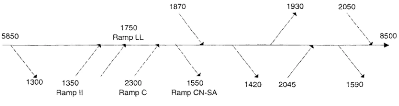
The Network used in the current study is a part of the Central Artery/ Tunnel(CA/T) Project in Boston. It is a 7.5 mile highway, approximately half of which will be built as a tunnel. The two parts of the network used in the current study are 1-90 West and 1-93 North. This part of 1-90 West is also called the Ted Williams Tunnel. It is a two lane 1.6 mile stretch of tunnel with loop detectors at every 200ft. Speed traps are located at every 600 ft. 1-90 West is a simple 2-lane tunnel with no geometric change. As discussed in the earlier section, the problem of detecting incidents in this simple network configuration reduces to that of detecting congestion. The results,presented later, support this claim. The 1-93 North varies between 3 and 4 lanes. Loop detectors are located at every 600 ft on normal freeways and at every 200ft in the tunnel. There are 6 on-ramps and 5 off-ramps. The locations of these ramps are shown in Figure 2-1. The flow rates on the different links in Figure 2-1 are based on the OD flows estimated for the year 2004 during the PM peak. This

1870 5850 1300 1350 Ramp 11 1750 Ramp LL 1930 / / / / .7 2300 Ramp C 1550 Ramp CN-SA 1420 / / / / / 2045 2050 8500 1590

Figure 2-1: 1-93 North Bound

demand is provided by the CA/T project and is used as the base demand(100%) for scenario design. Sensor data is generated for all stations on 1-93 North and analyzed for presence of incidents. There are significant variations in geometry because of on- and off- ramps, add/drop lanes and curvature.

2.2

The McMaster Algorithm

The McMaster algorithm uses flow-occupancy data to classify the traffic conditions into different states based on pre-determined thresholds. A typical fundamental diagram has been presented in Figure 2-2. The parameters OCMAX, VCRIT and the shape of the curve have to be determined

VCRIT

Region IV

Region I

Region II Region III

6CMAX

Occupancy

Figure 2-2: Fundamental Diagram of Traffic Flow

before the algorithm can be used. The algorithm uses the flow and occupancy values to classify the current traffic state as one of the four states shown in Figure2-2. Based on this classification, the algorithm decides if incident conditions exist at a particular sensor station. Region I represents a

region of low occupancy and flow varying from low to high. This represents an incident-free con-dition. Region II is a region of low flow at low occupancies. This typically represents the traffic state at a sensor station downstream of a blocked lane. Region III is the other type of incident state. It represents a high occupancy and low flow state. This is the traffic state upstream of the blocked lane. Region IV is a high occupancy, high flow region. This is typically the state downstream of a permanent bottleneck, e.g. an on-ramp. The parameters of the flow-occupancy plot have to be calibrated.

The McMaster algorithm seeks to ensure that the data in the congested regime can be clearly separated from other random fluctuations. The essence of the McMaster algorithm is that it tries to explain sudden discrete changes in one variable when other related variables are exhibiting smooth and continuous change. Further details can be obtained in Persaud et al.[7]. The Microscopic Traffic Simulator(MITSIM)[37] was used to generate the fundamental diagram by varying the OD flows. Zhou et al.[3 1], Hall et al. [12] and Hall et al.[13] have dealt extensively with the shape of the flow-occupancy and speed-flow plots. They have fitted different curves to the left portion of the flow-occupancy plot. Particularly, Zhou et al.[3 1] have estimated a cubic polynomial for the speed-flow plot. In order to better represent the overall flow-occupancy relationship, polynomials of different degrees were fitted to the data consisting of congested and uncongested operation. Two main criteria have been used to select the degree of interpolation.

i. Better representation of the overall relationship:- The fit can be used as a criterion to select

the best polynomial. Both r-squared and adjusted r-squared values have been used to decide best fit. Polynomials of degree 4 or higher were found to have better fit for most of the stations. However, the r-squared indicated an overfit after degree 4.

ii. Conservative representation of region II of the fundamental diagram:- The Region II of the

fundamental diagram is the state of traffic at a station downstream of an incident. The pa-rameter OCCmaX defines region II. It was identified that polynomials of degree 4 or higher conservatively define OCCma. making false identifications of incident harder. This reduces the FAS without affecting the DTR or TTD. Therefore these polynomials have been used. Table 2.1 is representative of the trend observed in OCCmax for different degrees of

interpo-lation.

Table 2.1: OCCma squared for different degrees

Degree OCCmax

2 23.86

3 23.55

4 21.58

5 21.58

The results from fitting different polynomials to the data for a sample sensor has been produced in Table 2.2. As indicated by the adjusted r-squared values in the table, the model becomes an overfit when the degree of the polynomial is 5. Thus the form of the polynomial used is

flow

+

+

The thresholds can be determined from the shape of the left portion of the curve. Some typical parameter values obtained from the simulation have been shown in Table 2.3. The initial

calibra-Table 2.2: R-square and Adjusted R-squared for different degrees

Degree R-squared Adjusted R-squared

2 0.7444 0.7420

3 0.7567 0.7557

4 0.7644 0.7607

5 0.7719 0.7605

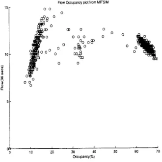
tion and testing of the algorithms was done for the Ted Williams Tunnel. Projected 2004 PM peak flows were used as the base flows. A typical plot generated from the simulation data has been presented in Figure 2-3. Once an n-degree polynomial is fitted to the data, the threshold curve (curve between 0 and OCCWC) is the 97.5% confidence curve. The threshold has been chosen so that 95% of the points fall above the threshold in the no incident case. A sample plot is shown in Figure 2-4.

0 0

0

S00 0

Flow Occupancy plot from MITSIM 0 0 0 OD 0 0 0 0 00 0 Oo 8 00 0 10 20 30 40 Occupancy(%) 0 0 0 0 -0 0 0 O 50 60 70

Figure 2-3: Flow Occupancy plot for a sensor

Table 2.3: Typical parameter values for a station for the McMaster algorithm

Parameter Value ao -2.5 a i 1.4 a2 -6.5x10-2 a3 1.2x10-3 a4 -7x10-6 OCCmax(in %) 21.58

Verit(in veh/30 sec) 13.5

Av.Spd.(in mph) 50

2.3

The APID Algorithm

The All Purpose Incident Detection algorithm(APID) uses a combination of different algorithms to identify incident conditions at different levels of flows ranging from low to high. The parameters have to be obtained by observing the values of the different measures used by the algorithm over a wide range of scenarios. Philip et al.[34] have presented the basic framework of the algorithm. However, they have used the same set of parameters for all the stations. They acknowledged that performance could be improved by using different groups of parameters. Their parameters are the initial values for the parameter calibration in our study. Calibration has helped identify different

15

10

0

16 14 12 10 8 5 10 15 20 25

Figure 2-4: Sample plot of McMaster threshold curve with the ±97.5% confidence curves groups of parameters for different stations. The calibration has been performed for sensors in both the Ted Williams Tunnel and the 1-93 North Bound. All stations in the Ted Williams tunnel have used the same set of parameters due its simple geometry. At a spacing of 200 ft, five different groups of parameters have been identified for 1-93 North. The algorithm uses three main routines

-a low volume routine, a medium volume routine and a high volume routine. The California Inci-dent detection algorithm is used as the high volume routine. The basic framework has been slightly modified for the current study. The basic algorithm uses compression wave testing and suspension of detection when compression waves are detected. Suspension of detection is used to reduce false alarms due to turbulent traffic conditions. Although it decrease FAS appreciably, it also directly affects detection rate. The incidents on 1-93 North have been placed in locations close to recurrent bottlenecks which are subject to turbulent traffic conditions. To avoid missed detection, suspension of detection has not been used in the present case. Suspension can always be replaced by higher thresholds and persistency checks for locations of unstable traffic conditions. The persistency of

3 polling periods has been found sufficient to eliminate compression wave testing at a spacing of

200ft. Persistency checking has also been applied to identify the end of the incident and return to normal traffic conditions. Typical parameter thresholds used by the different components of the

APID algorithm are presented in Table 2.5. Typical plots of the measures have been produced in

Figure 2-5 and Figure 2-6. Based on these plots, the thresholds for the different measures were decided.

Table 2.4: Measures used by the APID algorithm

Description Measure

Spatial difference in occ(OCCDF) occdf(i,t)=occ(i,t)-occ(i+ 1,t)

Relative spatial difference in occ(OCCRDF) occdf(i,t)/occ(i,t)

Relative temporal difference in d/s occ(DOCCTD) docctd(i,t)=(occ(i+1,t-2)-occ(i+1,t))/occ(i+1,t-2)

Downstream Occupancy(DOCC) docc(i,t)=occ(i+l,t)

Relative temporal diff in speed(SPDTDF) spdtdf(i,t)=(spd(i,t-2)-spd(i,t))/spd(i,t-2) Persistency threshold(PERSTH) threshold to be exceeded in persistency check Medium Traffic Threshold(MEDTRFTH) threshold to be exceeded to use med flow alg

Clearence Threshold(CLRTH) threshold to be exceeded to clear incident

(a) Incident- free (b) Incident

Table 2.5: Typical APID parameters

Calif Inc. Det. Med Vol Inc. Det Other prms

Prm Group DOCC OCCDF OCCRDF DOCCTD SPDTDF PERSTH MEDTRFTH CLRTH

1 20 25 0.35 0.40 0.10 0.35 15 0.31 2 17 15 0.65 0.40 0.10 0.65 15 0.31 3 17 55 0.80 0.40 0.10 0.80 15 0.31 4 17 30 0.50 0.40 0.10 0.50 15 0.31 5 17 20 0.50 0.40 0.10 0.50 15 0.31 0 So 000 1500 2W 2500 3000 3500 4

(a) Incident-free (b) Incident

Chapter 3

Evaluation of the McMaster and APID

algorithms

3.1

Refinements to the McMaster algorithm

Refinements for 1-90

Initial tests were conducted in the Ted William tunnel. The results of the tests indicated that algorithms were not directly transferable to networks with dense loop detector spacing. Incidents and other incident-like traffic states were easily detected which resulted in high number of false alarms. In order to clearly distinguish between incidents and other patterns similar to incidents, refinements were designed. These refinements were also tested in the second series of tests on 1-93 North.

Memory of true alarm to simulate actual behavior

The McMaster algorithm primarily uses the traffic state at a station to identify incidents. For a dense spacing of loop detectors, it is possible to identify the incident state due to an incident at several stations in the vicinity of the incident. This implies that it is possible to declare the same incident twice. Subsequent alarms from the same incident would have to be suppressed or recognized to be secondary alarms. Gall et al.[1] indicate that secondary alarms should be identified but do not present any strategy. To prevent this, we use the strategy of declaring an

incident only if it has not been declared before. We do this by checking to see if an incident state exists in the vicinity of the current station. If there is a confirmed incident state, we check if this is a true incident. An alarm has been identified to be a true alarm if it is declared a maximum time tmax after the actual occurrence. The value of tmax has been established emperically to be 5,7.5 and 10 minutes for spacing of 200ft, 600ft and 1200ft respectively. In real situations, this would correspond to the following. An operator is notified of an incident at a location. He/She responds to the alarm. If the alarm is true, an incident management plan is executed and any further alarms in the vicinity would be secondary. But if the alarm is a false alarm, the state of the station is restored to no incident. So, any further alarms in the vicinity would be(if they are not genuine) treated as false alarms. This strategy is one of the additions to the basic McMaster algorithm.

State Constraint

The original McMaster algorithm suggests that either Region I or Region II can be treated as incident state. For the close detector spacing in the tunnel, this was found to be inappropriate. This condition could be useful for larger sensor spacings. In order to reduce false alarms from this state, it was constrained that during the persistency check interval, the state 3 should be observed upstream of the incident(high density state) at least once. Incident should not be declared if over the entire persistency interval, only state 2 was observed at the station. It should be noted that a condition with state 3 upstream and state 2 downstream may occur for only one set of upstream and downstream stations. However, state 2 can be observed for many sensor station pairs both upstream and downstream of the incident. Gall et al.[l] proposed the original logic for a portion of the Queen Elizabeth Freeway where the spacing of loops is approximately 2200 ft. However, when the spacing is around 200-600 ft, incidents are hardly missed and numerous stations in the vicinity of the incident declare the incident if the state constraint is not imposed.

Count Constraint

The original algorithm does not use any basic reduction in flow. From preliminary investigations, it was found that for 30 sec polling period, there was a reduction in the count at the downstream station compared to the upstream station, at the end of the first polling period during which the

incident occurs. Therefore, it was constrained that for the first persistency check interval, the upstream count should be greater than the downstream count. This condition basically exploits the simple geometry of the Ted Williams Tunnel. For a 2 lane freeway stretch, flow discontinuities can easily be identified for small sensor data averaging periods and dense loop spacings.

Refinements to the McMaster algorithm for 1-93 North

The refinements used in the tunnel case were also applied to the 1-93 North. But it was found that the count constraint was too tight for the 3 lane and 4 lane case. Therefore this constraint was relaxed. However, the state constraint and the false alarm memory conditions were retained.

3.2

Refinements to the APID algorithm

The algorithm uses three main routines - a low volume routine, a medium volume routine and a high volume routine. The California Incident detection algorithm[ 11] is used as the high volume routine. The basic framework has been modified for the current study. The basic algorithm uses compression wave testing and suspension of detection when compression waves are detected. Sus-pension of detection has not been used in the present case. The persistency of 3 polling periods has been found sufficient to eliminate compression wave testing at a spacing of 200ft. Incident state at any station was reset only when the traffic variable values returned to normal for a specified number of consecutive time intervals. Thus, persistency checking was used to declare and clear the incidents.

3.3 Evaluation Results

3.3.1

Evaluation on 1-90 West

The network in this case consists of one OD pair. Flow rates were increased from 900 vphpl to 2000 vphpl in steps of 100 vphpl. The incident duration considered were 3 , 6 and 10 min. Thus, a total of 12*3 = 36 experiments were conducted. A total of 20 replications were performed per

experiment. For the different experiments, the incident location was fixed. The simple network geometry eliminates the need for studying different incident locations. The incident resulted in a one lane closure. A total of one hour of simulation was performed and the incident occurred at

10 minutes from the start of simulation. For all experiments, the polling period was 30 seconds

for both the algorithms. There were a total of 56 stations with 2 sensors each in this network. Therefore the total number of checks made by the algorithm in 20 hours of experiments with a polling period of 30 seconds was 120x20x56x2 = 268800. This number was used in computing the false alarm rate(= (FAS / number of checks)* 100). When the number of checks made by the algorithm becomes very high, the percentage of checks resulting in incident declarations become a very small fraction of the total. Expressing the false alarms as FAR therefore does not convey a correct idea of the actual number of false alarms. Therefore, both FAR and FAS(number of false alarms) have been presented. The results are presented in Table 3.2 and Table 3.3.

Analysis of tests on 1-90 West

Table 3.1: Original McMaster Algorithm, Persistency=3, Spacing=200ft

Inc. Duration Parameter 900 1000 1100 1200 1300 1400 1500 1600 TTD(min) 2.03 2.15 2.11 2.12 2.09 1.77 1.75 1.60 3 min DTR(%) 70 75 95 100 100 100 100 100 FAS 2 3 3 5 11 12 14 18 TTD(min) 2.23 2.21 2.24 2.02 2.10 1.85 1.73 1.58 6 min DTR(%) 65 80 90 95 100 100 100 100 FAS 5 4 8 10 18 19 22 24 TTD(min) 2.23 2.14 2.09 2.04 1.87 1.81 1.77 1.72 10 min DTR(%) 35 75 95 100 100 100 100 100 FAS 8 6 11 14 24 27 31 34

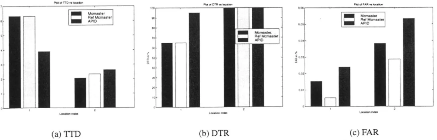
i. As depicted in Figure 3-1 and Figure 3-2, APID outperforms the McMaster algorithm. The components of APID are algorithms based on comparative logic. Such algorithms are known to have problems in presence of significant changes in geometry[7]. Since 1-90 West is a fairly straight tunnel stretch with almost no variation in geometry, APID has good perfor-mance. In the second set of tests on 1-93, it will be seen that the APID algorithm has poor performance at greater sensor spacings when there are substantial changes in geometry.

Table 3.2: Refined McMaster Algorithm, Persistency=3, Spacing=200ft

Inc. Duration Parameter 900 1000 1100 1200 1300 1400 1500 1600 TTD(min) 2.09 2.18 2 2.05 2.16 1.8 1.8 1.75 3 min DTR(%) 55 70 95 95 95 100 100 100 FAS 0 1 2 1 1 2 2 3 TTD(min) 2.83 2.53 2.24 2 2.08 1.95 1.92 1.85 6 min DTR(%) 45 70 85 95 95 100 100 100 FAS 0 2 1 2 3 4 4 4 TTD(min) 2.2 2.25 2.23 2.2 2.18 1.98 1.95 1.8 10 min DTR(%) 25 70 90 100 100 100 100 100 FAS 1 2 4 6 5 8 12 16

Table 3.3: APID algorithm, Persistency=3, Spacing=200ft

Inc. Duration Parameter 900 1000 1100 1200 1300 1400 1500 1600 TTD(min) 2.00 2.37 2.08 2.03 1.90 1.63 1.58 1.55 3 min DTR(%) 30 75 100 100 100 100 100 100 FAS 0 1 0 0 0 1 0 0 TTD(min) 3.50 2.81 2.13 1.94 1.78 1.60 1.60 1.58 6 min DTR(%) 45 90 100 100 100 100 100 100 FAS 0 1 0 0 1 0 0 2 TTD(min) 2.91 2.00 1.71 1.65 1.60 1.50 1.50 1.50 10 min DTR(%) 85 95 100 100 100 100 100 100 FAS 0 1 1 3 2 2 5 9

ii. The McMaster in its original form has a high number of false alarms. This can be attributed

to the fact that the algorithm in its original form does not effectively distinguish between incident and other forms of congestion when the spacing is 200 ft. The heuristics help identify incidents clearly. Some scenarios even have a FAS of 0 at low flow rates. These results are very similar to the findings of Peeta and Das[39].

iii. Both algorithms have extremely good performance with respect to false alarms. However,

as mentioned in earlier sections, these results are misleading and do not represent the per-formance under a general set of conditions. In the second set of experiments on 1-93 North in the next section, it will be shown that the performance deteriorates drastically in a more complex network.

I...

L~212

40-o

2 4 e a .s 12 14 16 Is 2 e 100 io 2W Mc 14W0 150 1I0N

(a) DTR vs FAS (b) FAS vs Flow rate

Figure 3-1: Plot of MOEs

F---(a) DTR vs Flow rate (b) TTD vs Flow rate

Figure 3-2: Plot of MOEs

3.3.2 Evaluation on 1-93 North

Experiments on 1-93 North

Incidents were placed at 2 locations. A total of 20 replications, each of 1.5 hrs were simulated. The OD flow of 2004PM was used as the base flow. The Incidents were simulated to occur 10 minutes after the beginning of the simulation and lasted 15 minutes. A complete lane blockage of the center lane in a 3 lane section was considered for location 1 and a complete blockage of the second lane from the left of a 4 lane section. The total number of stations in the present case is 74. The stations consist of both 3 and 4 lane sections (correspondingly 3 and 4 sensors). Therefore the total number of checks made by the algorithm in 20 experiments of 1.5 hr each with a polling

period of 30 seconds is 180x20x300(total number of sensors) = 1080000 at 200ft spacing, 360000

at 600ft spacing and 180000 at 1200ft spacing. The refinements used for the 1-90 West case were also applied to the 1-93 North. But it was found that the count constraint was too tight for the 3 lane and 4 lane case. This resulted in many missed detections. Therefore this constraint was relaxed. However, the state constraint and the false alarm memory conditions were retained. Unlike the Ted Williams tunnel, incident alarms were observed before the incidents in some replications. The results have been presented in Table 3.4 to Table 3.1.

i. Location ] -South of 1-90, downstream of ramp LL and upstream of ramp C.

Location 1 on 1-93 NB mainline

1950 ft 1100 ft Location 2 on 1-93NB mainline

1100 ft 1700 ft

X

Ramp LL Ramp Ramp C Ramp CN-SA

X - Incident Location X - incident location

(a) Location 1 (b) Location 2

Figure 3-3: Incident Locations

ii. Location 2 -In the weaving section, downstream of ramp C and upstream of ramp CN-SA. This congestion in this section builds up at a much faster rate than location 1.