Deep Captioning with Multimodal Recurrent Neural Networks (m-RNN)

Deep Captioning with Multimodal Recurrent

Neural Networks (m-RNN)

by

Junhua Mao, Wei Xu, Yi Yang, Jiang Wang, Zhiheng Huang, Alan L. Yuille

Abstract

In this paper, we present a multimodal Recurrent Neural Network (m-RNN) model for generating novel image captions. It directly models the probability distribution of generating a word given previous words and an image. Image captions are generated according to this distribution. The model con-sists of two sub-networks: a deep recurrent neural network for sentences and a deep convolutional network for images. These two sub-networks interact with each other in a multimodal layer to form the whole m-RNN model. The effectiveness of our model is validated on four benchmark datasets (IAPR TC-12, Flickr 8K, Flickr 30K and MS COCO). Our model outperforms the state-of-the-art methods. In addition, the m-RNN model can be applied to retrieval tasks for retrieving images or sentences, and achieves significant performance improvement over the state-of-the-art methods which directly optimize the ranking objective function for retrieval.

This work was supported by the Center for Brains, Minds and

Ma-chines (CBMM), funded by NSF STC award CCF - 1231216.

D

EEP

C

APTIONING WITH

M

ULTIMODAL

R

ECURRENT

N

EURAL

N

ETWORKS

(

M

-RNN)

Junhua Mao

University of California, Los Angeles; Baidu Research mjhustc@ucla.edu

Wei Xu & Yi Yang & Jiang Wang & Zhiheng Huang Baidu Research

{wei.xu,yangyi05,wangjiang03,huangzhiheng}@baidu.com Alan Yuille

University of California, Los Angeles yuille@stat.ucla.edu

A

In this paper, we present a multimodal Recurrent Neural Network (m-RNN) model for generating novel image captions. It directly models the probability distribution of generating a word given previous words and an image. Image captions are generated according to this distribution. The model consists of two sub-networks: a deep recurrent neural network for sentences and a deep convolutional network for images. These two sub-networks interact with each other in a multimodal layer to form the whole m-RNN model. The effectiveness of our model is validated on four benchmark datasets (IAPR TC-12, Flickr 8K, Flickr 30K and MS COCO). Our model outperforms the state-of-the-art methods. In addition, the m-RNN model can be applied to retrieval tasks for retrieving images or sentences, and achieves significant performance improvement over the state-of-the-art methods which directly optimize the ranking objective function for retrieval.1

1 I

Obtaining sentence level descriptions for images is becoming an important task and it has many ap-plications, such as early childhood education, image retrieval, and navigation for the blind. Thanks to the rapid development of computer vision and natural language processing technologies, recent work has made significant progress on this task (see a brief review in Section 2). Many previous methods treat it as a retrieval task. They learn a joint embedding to map the features of both sen-tences and images to the same semantic space. These methods generate image captions by retrieving them from a sentence database. Thus, they lack the ability of generating novel sentences or describ-ing images that contain novel combinations of objects and scenes.

In this work, we propose a multimodal Recurrent Neural Networks (m-RNN) model2 _{to address} both the task of generating novel sentences descriptions for images, and the task of image and sentence retrieval. The whole m-RNN model contains a language model part, a vision part and a multimodal part. The language model part learns a dense feature embedding for each word in the dictionary and stores the semantic temporal context in recurrent layers. The vision part contains a deep Convolutional Neural Network (CNN) which generates the image representation. The multi-modal part connects the language model and the deep CNN together by a one-layer representation.

1_{The project page of this work is: www.stat.ucla.edu/˜junhua.mao/m-RNN.html}

2_{A previous version of this work appears in the NIPS 2014 Deep Learning Workshop with the title “Explain} Images with Multimodal Recurrent Neural Networks” http://arxiv.org/abs/1410.1090 (Mao et al. (2014)). We observed subsequent arXiv papers which also use recurrent neural networks in this topic and cite our work. We gratefully acknowledge them.

R et r. G en .

1. Tourists are sitting at a long table with beer bottles on it in a rather dark restaurant and are raising their bierglaeser; 2. Tourists are sitting at a long table with a white table-cloth in a somewhat dark restaurant;

Tourists are sitting at a long table with a white table cloth and are eating;

1. Top view of the lights of a city at night, with a well-illuminated square in front of a church in the foreground; 2. People on the stairs in front of an illuminated cathedral with two towers at night;

A square with burning street lamps and a street in the foreground;

1. A dry landscape with light brown grass and green shrubs and trees in the foreground and large reddish-brown rocks and a blue sky in the background; 2. A few bushes at the bottom and a clear sky in the background; A dry landscape with green trees and bushes and light brown grass in the foreground and reddish-brown round rock domes and a blue sky in the background;

1. Group picture of nine tourists and one local on a grey rock with a lake in the background;

2. Five people are standing and four are squatting on a brown rock in the foreground;

A blue sky in the background;

Figure 1: Examples of the generated and two top-ranked retrieved sentences given the query image from IAPR TC-12 dataset. The sentences can well describe the content of the images. We show a failure case in the fourth image, where the model mistakenly treats the lake as the sky and misses all the people. More examples from the MS COCO dataset can be found on the project page: www.stat.ucla.edu/˜junhua.mao/m-RNN.html.

Our m-RNN model is learned using a log-likelihood cost function (see details in Section 4). The errors can be backpropagated to the three parts of the m-RNN model to update the model parameters simultaneously.

In the experiments, we validate our model on four benchmark datasets: IAPR TC-12 (Grubinger et al. (2006)), Flickr 8K (Rashtchian et al. (2010)), Flickr 30K (Young et al. (2014)) and MS COCO (Lin et al. (2014)). We show that our method achieves state-of-the-art performance, significantly outperforming all the other methods for the three tasks: generating novel sentences, retrieving im-ages given a sentence and retrieving sentences given an image. Our framework is general and can be further improved by incorporating more powerful deep representations for images and sentences.

2 R

W

Deep model for computer vision and natural language. The methods based on the deep neural network developed rapidly in recent years in both the field of computer vision and natural lan-guage. For computer vision, Krizhevsky et al. (2012) propose a deep Convolutional Neural Net-works (CNN) with 8 layers (denoted as AlexNet) and outperform previous methods by a large margin in the image classification task of ImageNet challenge (Russakovsky et al. (2014)). This network structure is widely used in computer vision, e.g. Girshick et al. (2014) design a object de-tection framework (RCNN) based on this work. Recently, Simonyan & Zisserman (2014) propose a CNN with over 16 layers (denoted as VggNet) and performs substantially better than the AlexNet. For natural language, the Recurrent Neural Network (RNN) shows the state-of-the-art performance in many tasks, such as speech recognition and word embedding learning (Mikolov et al. (2010; 2011; 2013)). Recently, RNNs have been successfully applied to machine translation to extract semantic information from the source sentence and generate target sentences (e.g. Kalchbrenner & Blunsom (2013), Cho et al. (2014) and Sutskever et al. (2014)).

Image-sentence retrieval. Many previous methods treat the task of describing images as a retrieval task and formulate the problem as a ranking or embedding learning problem (Hodosh et al. (2013); Frome et al. (2013); Socher et al. (2014)). They first extract the word and sentence features (e.g. Socher et al. (2014) uses dependency tree Recursive Neural Network to extract sentence features) as well as the image features. Then they optimize a ranking cost to learn an embedding model that maps both the sentence feature and the image feature to a common semantic feature space. In this way, they can directly calculate the distance between images and sentences. Recently, Karpathy et al. (2014) show that object level image features based on object detection results can generate better results than image features extracted at the global level.

Generating novel sentence descriptions for images. There are generally three categories of meth-ods for this task. The first category assumes a specific rule of the language grammar. They parse

(b). The m-RNN model

Embedding I Embedding II Recurrent Multimodal SoftMax

wstart Image CNN w1 Image CNN wL Image CNN

...

(a). The simple RNN model

w(t) r(t-1) r(t) y(t) w(t-1)

...

The m-RNN model for one time frame

128 256 256 512

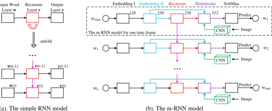
Figure 2: Illustration of the simple Recurrent Neural Network (RNN) and our multimodal Recurrent Neural Network (m-RNN) architecture. (a). The simple RNN. (b). Our m-RNN model. The inputs of our model are an image and its corresponding sentence descriptions. w1, w2, ..., wLrepresents the words in a sentence. We add a start sign wstartand an end sign wendto all the training sentences. The model estimates the probability distribution of the next word given previous words and the image. It consists of five layers (i.e. two word embedding layers, a recurrent layer, a multimodal layer and a softmax layer) and a deep CNN in each time frame. The number above each layer indicates the dimension of the layer. The weights are shared among all the time frames. (Best viewed in color) the sentence and divide it into several parts (Mitchell et al. (2012); Gupta & Mannem (2012)). Each part is associated with an object or an attribute in the image (e.g. Kulkarni et al. (2011) uses a Con-ditional Random Field model and Farhadi et al. (2010) uses a Markov Random Field model). This kind of method generates sentences that are syntactically correct. The second category retrieves similar captioned images, and generates new descriptions by generalizing and composing the re-trieved captions (Kuznetsova et al. (2014)). The third category of methods, which is more related to our method, learns a probability density over the space of multimodal inputs (i.e. sentences and images), using for example, Deep Boltzmann Machines (Srivastava & Salakhutdinov (2012)), and topic models (Barnard et al. (2003); Jia et al. (2011)). They generate sentences with richer and more flexible structure than the first group. The probability of generating sentences using the model can serve as the affinity metric for retrieval. Our method falls into this category. More closely related to our tasks and method is the work of Kiros et al. (2014b), which is built on a Log-BiLinear model (Mnih & Hinton (2007)) and use AlexNet to extract visual features. It needs a fixed length of context (i.e. five words), whereas in our model, the temporal context is stored in a recurrent architecture, which allows arbitrary context length.

Shortly after Mao et al. (2014), several papers appear with record breaking results (e.g. Kiros et al. (2014a); Karpathy & Fei-Fei (2014); Vinyals et al. (2014); Donahue et al. (2014); Fang et al. (2014); Chen & Zitnick (2014)). Many of them are built on recurrent neural networks. It demonstrates the effectiveness of storing context information in a recurrent layer. Our work has two major difference from these methods. Firstly, we incorporate a two-layer word embedding system in the m-RNN network structure which learns the word representation more efficiently than the single-layer word embedding. Secondly, we do not use the recurrent layer to store the visual information. The image representation is inputted to the m-RNN model along with every word in the sentence description. It utilizes of the capacity of the recurrent layer more efficiently, and allows us to achieve state-of-the-art performance using a relatively small dimensional recurrent layer. In the experiments, we show that these two strategies lead to better performance. Our method is still the best-performing approach for almost all the evaluation metrics.

3 M

A

3.1 SIMPLE RECURRENT NEURAL NETWORK

We briefly introduce the simple Recurrent Neural Network (RNN) or Elman network (Elman (1990)). Its architecture is shown in Figure 2(a). It has three types of layers in each time frame:

the input word layer w, the recurrent layer r and the output layer y. The activation of input, re-current and output layers at time t is denoted as w(t), r(t), and y(t) respectively. w(t) denotes the current word vector, which can be a simple 1-of-N coding representation h(t) (i.e. the one-hot representation, which is binary and has the same dimension as the vocabulary size with only one non-zero element) Mikolov et al. (2010). y(t) can be calculated as follows:

x(t) = [w(t) r(t_{− 1)]; r(t) = f}1(U· x(t)); y(t) = g1(V· r(t)); (1) where x(t) is a vector that concatenates w(t) and r(t −1), f1(.)and g1(.)are element-wise sigmoid and softmax function respectively, and U, V are weights which will be learned.

The size of the RNN is adaptive to the length of the input sequence. The recurrent layers connect the sub-networks in different time frames. Accordingly, when we do backpropagation, we need to propagate the error through recurrent connections back in time (Rumelhart et al. (1988)).

3.2 OUR M-RNNMODEL

The structure of our multimodal Recurrent Neural Network (m-RNN) is shown in Figure 2(b). It has five layers in each time frame: two word embedding layers, the recurrent layer, the multimodal layer, and the softmax layer).

The two word embedding layers embed the one-hot input into a dense word representation. It en-codes both the syntactic and semantic meaning of the words. The semantically relevant words can be found by calculating the Euclidean distance between two dense word vectors in embedding layers. Most of the sentence-image multimodal models (Karpathy et al. (2014); Frome et al. (2013); Socher et al. (2014); Kiros et al. (2014b)) use pre-computed word embedding vectors as the initialization of their model. In contrast, we randomly initialize our word embedding layers and learn them from the training data. We show that this random initialization is sufficient for our architecture to generate the state-of-the-art result. We treat the activation of the word embedding layer II (see Figure 2(b)) as the final word representation, which is one of the three direct inputs of the multimodal layer. After the two word embedding layers, we have a recurrent layer with 256 dimensions. The calcula-tion of the recurrent layer is slightly different from the calculacalcula-tion for the simple RNN. Instead of concatenating the word representation at time t (denoted as w(t)) and the recurrent layer activation at time t − 1 (denoted as r(t − 1)), we first map r(t − 1) into the same vector space as w(t) and add them together:

r(t) = f2(Ur· r(t − 1) + w(t)); (2)

where “+” represents element-wise addition. We set f2(.)to be the Rectified Linear Unit (ReLU), inspired by its the recent success when training very deep structure in computer vision field (Nair & Hinton (2010); Krizhevsky et al. (2012)). This differs from the simple RNN where the sigmoid function is adopted (see Section 3.1). ReLU is faster, and harder to saturate or overfit the data than non-linear functions like the sigmoid. When the backpropagation through time (BPTT) is conducted for the RNN with sigmoid function, the vanishing or exploding gradient problem appears since even the simplest RNN model can have a large temporal depth3_{. Previous work (Mikolov et al. (2010;} 2011)) use heuristics, such as the truncated BPTT, to avoid this problem. The truncated BPTT stops the BPTT after k time steps, where k is a hand-defined hyperparameter. Because of the good properties of ReLU, we do not need to stop the BPTT at an early stage, which leads to better and more efficient utilization of the data than the truncated BPTT.

After the recurrent layer, we set up a 512 dimensional multimodal layer that connects the language model part and the vision part of the m-RNN model (see Figure 2(b)). This layer has three inputs: the word-embedding layer II, the recurrent layer and the image representation. For the image rep-resentation, here we use the activation of the 7th_{layer of AlexNet (Krizhevsky et al. (2012)) or 15}th layer of VggNet (Simonyan & Zisserman (2014)), though our framework can use any image fea-tures. We map the activation of the three layers to the same multimodal feature space and add them together to obtain the activation of the multimodal layer:

m(t) = g2(Vw· w(t) + Vr· r(t) + VI· I); (3)

3_{We tried Sigmoid and Scaled Hyperbolic Tangent function as the non-linear functions for RNN in the}

where “+” denotes element-wise addition, m denotes the multimodal layer feature vector, I denotes the image feature. g2(.)is the element-wise scaled hyperbolic tangent function (LeCun et al. (2012)):

g2(x) = 1.7159· tanh( 2

3x) (4)

This function forces the gradients into the most non-linear value range and leads to a faster training process than the basic hyperbolic tangent function.

Both the simple RNN and m-RNN models have a softmax layer that generates the probability dis-tribution of the next word. The dimension of this layer is the vocabulary size M, which is different for different datasets.

4 T

-RNN

To train our m-RNN model we adopt a log-likelihood cost function. It is related to the Perplexity of the sentences in the training set given their corresponding images. Perplexity is a standard measure for evaluating language model. The perplexity for one word sequence (i.e. a sentence) w1:L is calculated as follows: log2PPL(w1:L|I) = − 1 L L X n=1 log2P (wn|w1:n−1, I) (5)

where L is the length of the word sequence, PPL(w1:L|I) denotes the perplexity of the sentence w1:Lgiven the image I. P (wn|w1:n−1, I)is the probability of generating the word wngiven I and previous words w1:n−1. It corresponds to the activation of the SoftMax layer of our model.

The cost function of our model is the average log-likelihood of the words given their context words and corresponding images in the training sentences plus a regularization term. It can be calculated by the perplexity: C =_N1 Ns X i=1 Li· log2PPL(w (i) 1:Li|I (i)_{) + λ} θ· kθk22 (6)

where Ns and N denotes the number of sentences and the number of words in the training set receptively, Lidenotes the length of ithsentences, and θ represents the model parameters.

Our training objective is to minimize this cost function, which is equivalent to maximize the proba-bility of generating the sentences in the training set using the model. The cost function is differen-tiable and we use backpropagation to learn the model parameters.

5 S

G

, I

R

S

R

We use the trained m-RNN model for three tasks: 1) Sentences generation, 2) Image retrieval (re-trieving most relevant images to the given sentence), 3) Sentence retrieval (re(re-trieving most relevant sentences to the given image).

The sentence generation process is straightforward. Starting from the start sign wstartor arbitrary number of reference words (e.g. we can input the first K words in the reference sentence to the model and then start to generate new words), our model can calculate the probability distribution of the next word: P (wn|w1:n−1, I). Then we can sample from this probability distribution to pick the next word. In practice, we find that selecting the word with the maximum probability performs slightly better than sampling. After that, we input the picked word to the model and continue the process until the model outputs the end sign wend.

For the retrieval tasks, we use our model to calculate the probability of generating a sentence w1:L given an image I: P (w1:L|I) =Q_nP (wn|w1:n−1, I). The probability can be treated as an affinity measurement between sentences and images.

For the image retrieval task, given the query sentence wQ

1:L, we rank the dataset images ID accord-ing to the probability P (wQ

1:L|ID)and retrieved the top ranked images. This is equivalent to the perplexity-based image retrieval in Kiros et al. (2014b).

The sentence retrieval task is trickier because there might be some sentences that have high proba-bility or perplexity for any image query (e.g. sentences consist of many frequently appeared words). To solve this problem, Kiros et al. (2014b) uses the perplexity of a sentence conditioned on the averaged image feature across the training set as the reference perplexity to normalize the original perplexity. Different from them, we use the normalized probability where the normalization factor is the marginal probability of wD

1:L: P (w1:LD |IQ)/P (wD1:L); P (w1:LD ) =PI0P (w D 1:L|I 0 )_{· P (I}0) (7) where wD

1:Ldenotes the sentence in the dataset, IQ denotes the query image, and I 0

are images sampled from the training set. We approximate P (I0

)by a constant and ignore this term. This strategy leads to a much better performance than that in Kiros et al. (2014b) in the experiments. The normalized probability is equivalent to the probability P (IQ

|wD

1:L), which is symmetric to the probability P (wQ

1:L|ID)used in the image retrieval task.

6 L

S

I

F

The architecture of our model allows the gradients from the loss function to be backpropagated to both the language modeling part (i.e. the word embedding layers and the recurrent layer) and the vision part (e.g. the AlexNet or VGGNet).

For the language part, as mentioned above, we randomly initialize the language modeling layers and learn their parameters. For the vision part, we use the pre-trained AlexNet (Krizhevsky et al. (2012)) or the VggNet (Simonyan & Zisserman (2014)) on ImageNet dataset (Russakovsky et al. (2014)). Recently, Karpathy et al. (2014) show that using the RCNN object detection results (Girshick et al. (2014)) combined with the AlexNet features performs better than simply treating the image as a whole frame. In the experiments, we show that our method performs much better than Karpathy et al. (2014) when the same image features are used, and is better than or comparable to their results even when they use more sophisticated features based on object detection.

We can update the CNN in the vision part of our model according to the gradient backpropagated from the multimodal layer. In this paper, we fix the image features and the deep CNN network in the training stage due to a shortage of data. In future work, we will apply our method on large datasets (e.g. the complete MS COCO dataset, which has not yet been released) and finetune the parameters of the deep CNN network in the training stage.

The m-RNN model is trained using Baidu’s internal deep learning platform PADDLE, which allows us to explore many different model architectures in a short period. The hyperparameters, such as layer dimensions and the choice of the non-linear activation functions, are tuned via cross-validation on Flickr8K dataset and are then fixed across all the experiments. It takes 25 ms on average to generate a sentence (excluding image feature extraction stage) on a single core CPU.

7 E

7.1 DATASETS

We test our method on four benchmark datasets with sentence level annotations: IAPR TC-12 (Grub-inger et al. (2006)), Flickr 8K (Rashtchian et al. (2010)), Flickr 30K (Young et al. (2014)) and MS COCO (Lin et al. (2014)).

IAPR TC-12. This dataset consists of around 20,000 images taken from different locations around the world. It contains images of different sports and actions, people, animals, cities, landscapes, etc. For each image, it provides at least one sentence annotation. On average, there are about 1.7 sentence annotations for one image. We adopt the standard separation of training and testing set as previous works (Guillaumin et al. (2010); Kiros et al. (2014b)) with 17,665 images for training and 1962 images for testing.

Flickr8K. This dataset consists of 8,000 images extracted from Flickr. For each image, it provides five sentence annotations. We adopt the standard separation of training, validation and testing set provided by the dataset. There are 6,000 images for training, 1,000 images for validation and 1,000 images for testing.

Flickr30K. This dataset is a recent extension of Flickr8K. For each image, it also provides five sentences annotations. It consists of 158,915 crowd-sourced captions describing 31,783 images. The grammar and style for the annotations of this dataset is similar to Flickr8K. We follow the previous work (Karpathy et al. (2014)) which used 1,000 images for testing. This dataset, as well as the Flick8K dataset, were originally used for the image-sentence retrieval tasks.

MS COCO. The current release of this recently proposed dataset contains 82,783 training images and 40,504 validation images. For each image, it provides five sentences annotations. We randomly sampled 4,000 images for validation and 1,000 images for testing from their currently released validation set. The dataset partition of MS COCO and Flickr30K is available in the project page4_.

7.2 EVALUATION METRICS

Sentence Generation. Following previous works, we use the sentence perplexity (see Equ. 5) and BLEU scores (i.e. B-1, B-2, B-3, and B-4) (Papineni et al. (2002)) as the evaluation metrics. BLEU scores were originally designed for automatic machine translation where they rate the quality of a translated sentences given several references sentences. Similarly, we can treat the sentence gener-ation task as the “translgener-ation” of the content of images to sentences. BLEU remains the standard evaluation metric for sentence generation methods for images, though it has drawbacks. For some images, the reference sentences might not contain all the possible descriptions in the image and BLEU might penalize some correctly generated sentences. Please see more details of the calcula-tion of BLEU scores for this task in the supplementary material seccalcula-tion 9.35_.

Sentence Retrieval and Image Retrieval. We adopt the same evaluation metrics as previous works (Socher et al. (2014); Frome et al. (2013); Karpathy et al. (2014)) for both the tasks of sentences retrieval and image retrieval. We use R@K (K = 1, 5, 10) as the measurement. R@K is the recall rate of a correctly retrieved groundtruth given top K candidates. Higher R@K usually means better retrieval performance. Since we care most about the top-ranked retrieved results, the R@K scores with smaller K are more important.

The Med r is another metric we use, which is the median rank of the first retrieved groundtruth sentence or image. Lower Med r usually means better performance. For IAPR TC-12 datasets, we use additional evaluation metrics to conduct a fair comparison with previous work (Kiros et al. (2014b)). Please see the details in the supplementary material section 9.3.

7.3 RESULTS ONIAPR TC-12

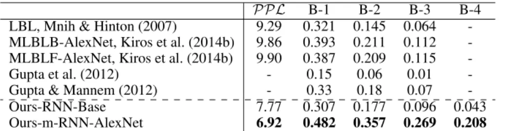
The results of the sentence generation task6 _{are shown in Table 1. Ours-RNN-Base serves as a} baseline method for our m-RNN model. It has the same architecture as m-RNN except that it does not have the image representation input.

To conduct a fair comparison, we follow the same experimental settings of Kiros et al. (2014b) to calculate the BLEU scores and perplexity. These two evaluation metrics are not necessarily correlated to each other for the following reasons. As mentioned in Section 4, perplexity is calculated according to the conditional probability of the word in a sentence given all of its previous reference words. Therefore, a strong language model that successfully captures the distributions of words in sentences can have a low perplexity without the image content. But the content of the generated sentences might be uncorrelated to images. From Table 1, we can see that although our baseline method of RNN generates a low perplexity, its BLEU score is low, indicating that it fails to generate sentences that are consistent with the content of images.

Table 1 shows that our m-RNN model performs much better than our baseline RNN model and the state-of-the-art methods both in terms of the perplexity and BLEU score.

4_{www.stat.ucla.edu/˜junhua.mao/m-RNN.html}

5_{The BLEU outputted by our implementation is slightly lower than the recently released MS COCO caption}

evaluation toolbox (Chen et al. (2015)) because of different tokenization methods of the sentences. We re-evaluate our method using the toolbox in the current version of the paper.

6_{Kiros et al. (2014b) further improved their results after the publication. We compare our results with their} updated ones here.

PPL B-1 B-2 B-3 B-4

LBL, Mnih & Hinton (2007) 9.29 0.321 0.145 0.064

-MLBLB-AlexNet, Kiros et al. (2014b) 9.86 0.393 0.211 0.112

-MLBLF-AlexNet, Kiros et al. (2014b) 9.90 0.387 0.209 0.115

-Gupta et al. (2012) - 0.15 0.06 0.01

-Gupta & Mannem (2012) - 0.33 0.18 0.07

-Ours-RNN-Base 7.77 0.307 0.177 0.096 0.043

Ours-m-RNN-AlexNet 6.92 0.482 0.357 0.269 0.208

Table 1: Results of the sentence generation task on the IAPR TC-12 dataset. “B” is short for BLEU. Sentence Retrival (Image to Text) Image Retrival (Text to Image)

R@1 R@5 R@10 Med r R@1 R@5 R@10 Med r

Ours-m-RNN 20.9 43.8 54.4 8 13.2 31.2 40.8 21

Table 2: R@K and median rank (Med r) for IAPR TC-12 dataset.

Sentence Retrival (Image to Text) Image Retrival (Text to Image)

R@1 R@5 R@10 Med r R@1 R@5 R@10 Med r Random 0.1 0.5 1.0 631 0.1 0.5 1.0 500 SDT-RNN-AlexNet 4.5 18.0 28.6 32 6.1 18.5 29.0 29 Socher-avg-RCNN 6.0 22.7 34.0 23 6.6 21.6 31.7 25 DeViSE-avg-RCNN 4.8 16.5 27.3 28 5.9 20.1 29.6 29 DeepFE-AlexNet 5.9 19.2 27.3 34 5.2 17.6 26.5 32 DeepFE-RCNN 12.6 32.9 44.0 14 9.7 29.6 42.5 15 Ours-m-RNN-AlexNet 14.5 37.2 48.5 11 11.5 31.0 42.4 15

Table 3: Results of R@K and median rank (Med r) for Flickr8K dataset. “-AlexNet” denotes the image representation based on AlexNet extracted from the whole image frame. “-RCNN” denotes the image representation extracted from possible objects detected by the RCNN algorithm.

For the retrieval tasks, since there are no publicly available results of R@K and Med r in this dataset, we report R@K scores of our method in Table 2 for future comparisons. The result shows that 20.9% top-ranked retrieved sentences and 13.2% top-ranked retrieved images are groundtruth. We also adopt additional evaluation metrics to compare our method with Kiros et al. (2014b), see sup-plementary material Section 9.2.

7.4 RESULTS ONFLICKR8K

This dataset was widely used as a benchmark dataset for image and sentence retrieval. The R@K and Med r of different methods are shown in Table 3. We compare our model with several state-of-the-art methods: SDT-RNN (Socher et al. (2014)), DeViSE (Frome et al. (2013)), DeepFE (Karpathy et al. (2014)) with various image representations. Our model outperforms these methods by a large margin when using the same image representation (e.g. AlexNet). We also list the performance of methods using more sophisticated features in Table 3. “-avg-RCNN” denotes methods with features of the average CNN activation of all objects above a detection confidence threshold. DeepFE-RCNN Karpathy et al. (2014) uses a fragment mapping strategy to better exploit the object detection results. The results show that using these features improves the performance. Even without the help from the object detection methods, however, our method performs better than these methods in almost all the evaluation metrics. We will develop our framework using better image features based on object detection in the future work.

The PPL, B-1, B-2, B-3 and B-4 of the generated sentences using our m-RNN-AlexNet model in this dataset are 24.39, 0.565, 0.386, 0.256, and 0.170 respectively.

Sentence Retrival (Image to Text) Image Retrival (Text to Image) R@1 R@5 R@10 Med r R@1 R@5 R@10 Med r Flickr30K Random 0.1 0.6 1.1 631 0.1 0.5 1.0 500 DeViSE-avg-RCNN 4.8 16.5 27.3 28 5.9 20.1 29.6 29 DeepFE-RCNN 16.4 40.2 54.7 8 10.3 31.4 44.5 13 RVR 12.1 27.8 47.8 11 12.7 33.1 44.9 12.5 MNLM-AlexNet 14.8 39.2 50.9 10 11.8 34.0 46.3 13 MNLM-VggNet 23.0 50.7 62.9 5 16.8 42.0 56.5 8 NIC 17.0 56.0 - 7 17.0 57.0 - 7 LRCN 14.0 34.9 47.0 11 - - - -DeepVS 22.2 48.2 61.4 4.8 15.2 37.7 50.5 9.2 Ours-m-RNN-AlexNet 18.4 40.2 50.9 10 12.6 31.2 41.5 16 Ours-m-RNN-VggNet 35.4 63.8 73.7 3 22.8 50.7 63.1 5 MS COCO Random 0.1 0.6 1.1 631 0.1 0.5 1.0 500 DeepVS-RCNN 29.4 62.0 75.9 2.5 20.9 52.8 69.2 4 Ours-m-RNN-VggNet 41.0 73.0 83.5 2 29.0 42.2 77.0 3

Table 4: Results of R@K and median rank (Med r) for Flickr30K dataset and MS COCO dataset.

Flickr30K MS COCO PPL B-1 B-2 B-3 B-4 PPL B-1 B-2 B-3 B-4 RVR - - - - 0.13 - - - - 0.19 DeepVS-AlexNet - 0.47 0.21 0.09 - - 0.53 0.28 0.15 -DeepVS-VggNet 21.20 0.50 0.30 0.15 - 19.64 0.57 0.37 0.19 -NIC - 0.66 - - - - 0.67 - - -LRCN - 0.59 0.39 0.25 0.16 - 0.63 0.44 0.31 0.21 DMSM - - - 0.21 Ours-m-RNN-AlexNet 35.11 0.54 0.36 0.23 0.15 - - - - -Ours-m-RNN-VggNet 20.72 0.60 0.41 0.28 0.19 13.60 0.67 0.49 0.35 0.25

Table 5: Results of generated sentences on the Flickr 30K dataset and MS COCO dataset.

Our m-RNN MNLM NIC LRCN RVR DeepVS

RNN Dim. 256 300 512 1000 (×4) 100 300-600

LSTM No Yes Yes Yes No No

Table 6: Properties of the recurrent layers for the five very recent methods. LRCN has a stack of four 1000 dimensional LSTM layers. We achieves state-of-the-art performance using a relatively small dimensional recurrent layer. LSTM (Hochreiter & Schmidhuber (1997)) can be treated as a sophisticated version of the RNN.

7.5 RESULTS ONFLICKR30KANDMS COCO

We compare our method with several state-of-the-art methods in these two recently released dataset (Note that the last six methods appear very recently, we use the results reported in their papers): DeViSE (Frome et al. (2013)), DeepFE (Karpathy et al. (2014)), MNLM (Kiros et al. (2014a)), DMSM (Fang et al. (2014)), NIC (Vinyals et al. (2014)), LRCN (Donahue et al. (2014)), RVR (Chen & Zitnick (2014)), and DeepVS (Karpathy & Fei-Fei (2014)). The results of the retrieval tasks and the sentence generation task7 _{are shown in Table 4 and Table 5 respectively. We also} summarize some of the properties of the recurrent layers adopted in the five very recent methods in Table 6.

7_{We only select the word with maximum probability each time in the sentence generation process in Table} 5 while many comparing methods (e.g. DMSM, NIC, LRCN) uses a beam search scheme that keeps the best K candidates. The beam search scheme will lead to better performance in practice using the same model.

B1 B2 B3 B4 CIDEr ROUGE L METEOR

m-RNN-greedy-c5 0.668 0.488 0.342 0.239 0.729 0.489 0.221

m-RNN-greedy-c40 0.845 0.730 0.598 0.473 0.740 0.616 0.291

m-RNN-beam-c5 0.680 0.506 0.369 0.272 0.791 0.499 0.225

m-RNN-beam-c40 0.865 0.760 0.641 0.529 0.789 0.640 0.304

Table 7: Results of the MS COCO test set evaluated by MS COCO evaluation server Our method with VggNet image representation (Simonyan & Zisserman (2014)) outperforms the state-of-the-art methods, including the very recently released methods, in almost all the evaluation metrics. Note that the dimension of the recurrent layer of our model is relatively small compared to the competing methods. It shows the advantage and efficiency of our method that directly inputs the visual information to the multimodal layer instead of storing it in the recurrent layer. The m-RNN model with VggNet performs better than that with AlexNet, which indicates the importance of strong image representations in this task. 71% of the generated sentences for MS COCO datasets are novel (i.e. different from training sentences).

We also validate our method on the test set of MS COCO by their evaluation server (Chen et al. (2015)). The results are shown in Table 7. We evaluate our model with greedy inference (select the word with the maximum probability each time) as well as with the beam search inference. “-c5” represents results using 5 reference sentences and “-c40” represents results using 40 reference sentences.

To further validate the importance of different components of the m-RNN model, we train sev-eral variants of the original m-RNN model and compare their performance. In particular, we show that the two-layer word embedding system outperforms the single-layer version and the strategy of directly inputting the visual information to the multimodal layer substantially improves the perfor-mance (about 5% for B-1). Due to the limited space, we put the details of these experiments in Section 9.1 in the supplementary material after the main paper.

8 C

We propose a multimodal Recurrent Neural Network (m-RNN) framework that performs at the state-of-the-art in three tasks: sentence generation, sentence retrieval given query image and image retrieval given query sentence. The model consists of a deep RNN, a deep CNN and these two sub-networks interact with each other in a multimodal layer. Our m-RNN is powerful of connecting images and sentences and is flexible to incorporate more complex image representations and more sophisticated language models.

ACKNOWLEDGMENTS

We thank Andrew Ng, Kai Yu, Chang Huang, Duohao Qin, Haoyuan Gao, Jason Eisner for useful discussions and technical support. We also thank the comments and suggestions of the anonymous reviewers from ICLR 2015 and NIPS 2014 Deep Learning Workshop. We acknowledge the Center for Minds, Brains and Machines (CBMM), partially funded by NSF STC award CCF-1231216, and ARO 62250-CS.

R

Barnard, Kobus, Duygulu, Pinar, Forsyth, David, De Freitas, Nando, Blei, David M, and Jordan, Michael I. Matching words and pictures. JMLR, 3:1107–1135, 2003.

Chen, Xinlei and Zitnick, C Lawrence. Learning a recurrent visual representation for image caption generation. arXiv preprint arXiv:1411.5654, 2014.

Chen, Xinlei, Fang, Hao, Lin, Tsung-Yi, Vedantam, Ramakrishna, Gupta, Saurabh, Dollr, Piotr, and Zitnick, C. Lawrence. Microsoft coco captions: Data collection and evaluation server. arXiv preprint arXiv:1504.00325, 2015.

Cho, Kyunghyun, van Merrienboer, Bart, Gulcehre, Caglar, Bougares, Fethi, Schwenk, Holger, and Bengio, Yoshua. Learning phrase representations using rnn encoder-decoder for statistical machine translation. arXiv preprint arXiv:1406.1078, 2014.

Donahue, Jeff, Hendricks, Lisa Anne, Guadarrama, Sergio, Rohrbach, Marcus, Venugopalan, Sub-hashini, Saenko, Kate, and Darrell, Trevor. Long-term recurrent convolutional networks for visual recognition and description. arXiv preprint arXiv:1411.4389, 2014.

Elman, Jeffrey L. Finding structure in time. Cognitive science, 14(2):179–211, 1990.

Fang, Hao, Gupta, Saurabh, Iandola, Forrest, Srivastava, Rupesh, Deng, Li, Doll´ar, Piotr, Gao, Jianfeng, He, Xiaodong, Mitchell, Margaret, Platt, John, et al. From captions to visual concepts and back. arXiv preprint arXiv:1411.4952, 2014.

Farhadi, Ali, Hejrati, Mohsen, Sadeghi, Mohammad Amin, Young, Peter, Rashtchian, Cyrus, Hock-enmaier, Julia, and Forsyth, David. Every picture tells a story: Generating sentences from images. In ECCV, pp. 15–29. 2010.

Frome, Andrea, Corrado, Greg S, Shlens, Jon, Bengio, Samy, Dean, Jeff, Mikolov, Tomas, et al. Devise: A deep visual-semantic embedding model. In NIPS, pp. 2121–2129, 2013.

Girshick, R., Donahue, J., Darrell, T., and Malik, J. Rich feature hierarchies for accurate object detection and semantic segmentation. In CVPR, 2014.

Grubinger, Michael, Clough, Paul, M¨uller, Henning, and Deselaers, Thomas. The iapr tc-12 bench-mark: A new evaluation resource for visual information systems. In International Workshop OntoImage, pp. 13–23, 2006.

Guillaumin, Matthieu, Verbeek, Jakob, and Schmid, Cordelia. Multiple instance metric learning from automatically labeled bags of faces. In ECCV, pp. 634–647, 2010.

Gupta, Ankush and Mannem, Prashanth. From image annotation to image description. In ICONIP, 2012.

Gupta, Ankush, Verma, Yashaswi, and Jawahar, CV. Choosing linguistics over vision to describe images. In AAAI, 2012.

Hochreiter, Sepp and Schmidhuber, J¨urgen. Long short-term memory. Neural computation, 9(8): 1735–1780, 1997.

Hodosh, Micah, Young, Peter, and Hockenmaier, Julia. Framing image description as a ranking task: Data, models and evaluation metrics. JAIR, 47:853–899, 2013.

Jia, Yangqing, Salzmann, Mathieu, and Darrell, Trevor. Learning cross-modality similarity for multinomial data. In ICCV, pp. 2407–2414, 2011.

Kalchbrenner, Nal and Blunsom, Phil. Recurrent continuous translation models. In EMNLP, pp. 1700–1709, 2013.

Karpathy, Andrej and Fei-Fei, Li. Deep visual-semantic alignments for generating image descrip-tions. arXiv preprint arXiv:1412.2306, 2014.

Karpathy, Andrej, Joulin, Armand, and Fei-Fei, Li. Deep fragment embeddings for bidirectional image sentence mapping. In arXiv:1406.5679, 2014.

Kiros, Ryan, Salakhutdinov, Ruslan, and Zemel, Richard S. Unifying visual-semantic embeddings with multimodal neural language models. arXiv preprint arXiv:1411.2539, 2014a.

Kiros, Ryan, Zemel, R, and Salakhutdinov, Ruslan. Multimodal neural language models. In ICML, 2014b.

Krizhevsky, Alex, Sutskever, Ilya, and Hinton, Geoffrey E. Imagenet classification with deep con-volutional neural networks. In NIPS, pp. 1097–1105, 2012.

Kulkarni, Girish, Premraj, Visruth, Dhar, Sagnik, Li, Siming, Choi, Yejin, Berg, Alexander C, and Berg, Tamara L. Baby talk: Understanding and generating image descriptions. In CVPR, 2011. Kuznetsova, Polina, Ordonez, Vicente, Berg, Tamara L, and Choi, Yejin. Treetalk: Composition and

compression of trees for image descriptions. TACL, 2(10):351–362, 2014.

LeCun, Yann A, Bottou, L´eon, Orr, Genevieve B, and M¨uller, Klaus-Robert. Efficient backprop. In Neural networks: Tricks of the trade, pp. 9–48. Springer, 2012.

Lin, Tsung-Yi, Maire, Michael, Belongie, Serge, Hays, James, Perona, Pietro, Ramanan, Deva, Doll´ar, Piotr, and Zitnick, C Lawrence. Microsoft coco: Common objects in context. arXiv preprint arXiv:1405.0312, 2014.

Mao, Junhua, Xu, Wei, Yang, Yi, Wang, Jiang, and Yuille, Alan L. Explain images with multimodal recurrent neural networks. arXiv preprint arXiv:1410.1090, 2014.

Mikolov, Tomas, Karafi´at, Martin, Burget, Lukas, Cernock`y, Jan, and Khudanpur, Sanjeev. Recur-rent neural network based language model. In INTERSPEECH, pp. 1045–1048, 2010.

Mikolov, Tomas, Kombrink, Stefan, Burget, Lukas, Cernocky, JH, and Khudanpur, Sanjeev. Exten-sions of recurrent neural network language model. In ICASSP, pp. 5528–5531, 2011.

Mikolov, Tomas, Sutskever, Ilya, Chen, Kai, Corrado, Greg S, and Dean, Jeff. Distributed represen-tations of words and phrases and their compositionality. In NIPS, pp. 3111–3119, 2013.

Mitchell, Margaret, Han, Xufeng, Dodge, Jesse, Mensch, Alyssa, Goyal, Amit, Berg, Alex, Ya-maguchi, Kota, Berg, Tamara, Stratos, Karl, and Daum´e III, Hal. Midge: Generating image descriptions from computer vision detections. In EACL, 2012.

Mnih, Andriy and Hinton, Geoffrey. Three new graphical models for statistical language modelling. In ICML, pp. 641–648. ACM, 2007.

Nair, Vinod and Hinton, Geoffrey E. Rectified linear units improve restricted boltzmann machines. In ICML, pp. 807–814, 2010.

Papineni, Kishore, Roukos, Salim, Ward, Todd, and Zhu, Wei-Jing. Bleu: a method for automatic evaluation of machine translation. In ACL, pp. 311–318, 2002.

Rashtchian, Cyrus, Young, Peter, Hodosh, Micah, and Hockenmaier, Julia. Collecting image anno-tations using amazon’s mechanical turk. In NAACL-HLT workshop 2010, pp. 139–147, 2010. Rumelhart, David E, Hinton, Geoffrey E, and Williams, Ronald J. Learning representations by

back-propagating errors. Cognitive modeling, 1988.

Russakovsky, Olga, Deng, Jia, Su, Hao, Krause, Jonathan, Satheesh, Sanjeev, Ma, Sean, Huang, Zhiheng, Karpathy, Andrej, Khosla, Aditya, Bernstein, Michael, Berg, Alexander C., and Fei-Fei, Li. ImageNet Large Scale Visual Recognition Challenge, 2014.

Simonyan, Karen and Zisserman, Andrew. Very deep convolutional networks for large-scale image recognition. arXiv preprint arXiv:1409.1556, 2014.

Socher, Richard, Le, Q, Manning, C, and Ng, A. Grounded compositional semantics for finding and describing images with sentences. In TACL, 2014.

Srivastava, Nitish and Salakhutdinov, Ruslan. Multimodal learning with deep boltzmann machines. In NIPS, pp. 2222–2230, 2012.

Sutskever, Ilya, Vinyals, Oriol, and Le, Quoc VV. Sequence to sequence learning with neural net-works. In NIPS, pp. 3104–3112, 2014.

Vinyals, Oriol, Toshev, Alexander, Bengio, Samy, and Erhan, Dumitru. Show and tell: A neural image caption generator. arXiv preprint arXiv:1411.4555, 2014.

Young, Peter, Lai, Alice, Hodosh, Micah, and Hockenmaier, Julia. From image descriptions to visual denotations: New similarity metrics for semantic inference over event descriptions. In ACL, pp. 479–488, 2014.

9 S

M

9.1 EFFECTIVENESS OF THE DIFFERENT COMPONENTS OF THE M-RNNMODEL

Embedding I Embedding II Recurrent Multimodal SoftMax wstart Image CNN Predict w1 The Original m-RNN model for one time frame

128 256 256 512 wstart Image CNN Predict w1 128 256 256 512 m-RNN-NoEmbInput wstart Image CNN Predict w1 256 256 512 m-RNN-OneLayerEmb wstart Image CNN Predict w1 128 256 256 512 m-RNN-EmbOneInput wstart Image CNN Predict w1 128 256 256 512 wstart Image CNN Predict w1 128 256 256 512 VI (1) VI (2) wstart Image CNN Predict w1 128 256 256 512 VI VI m-RNN-VisualInRnn m-RNN-VisualInRnn-Both m-RNN-VisualInRnn-Both-Shared

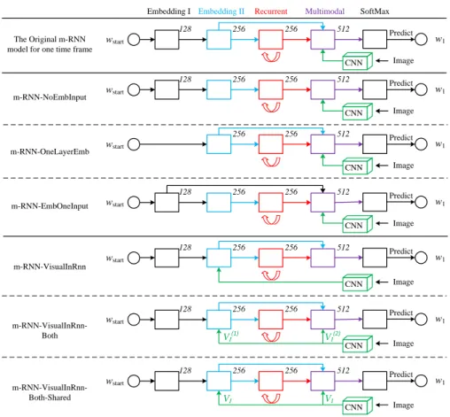
Figure 3: Illustration of the seven variants of the m-RNN models.

B-1 B-2 B-3 B-4 m-RNN 0.600 0.412 0.278 0.187 m-RNN-NoEmbInput 0.592 0.408 0.277 0.188 m-RNN-OneLayerEmb 0.594 0.406 0.274 0.184 m-RNN-EmbOneInput 0.590 0.406 0.274 0.185 m-RNN-visInRnn 0.466 0.267 0.157 0.101 m-RNN-visInRnn-both 0.546 0.333 0.191 0.120 m-RNN-visInRnn-both-shared 0.478 0.279 0.171 0.110

Table 8: Performance comparison of different versions of m-RNN models on the Flickr30K dataset. All the models adopt VggNet as the image representation. See Figure 3 for details of the models. In this section, we compare different variants of our m-RNN model to show the effectiveness of the two-layer word embedding and the strategy to input the visual information to the multimodal layer. The word embedding system. Intuitively, the two word embedding layers capture high-level se-mantic meanings of words more efficiently than the single layer word embedding. As an input to the multimodal layer, it offers useful information for predicting the next word distribution.

To validate its efficiency, we train three different m-RNN networks: NoEmbInput, m-RNN-OneLayerEmb, m-RNN-EmbOneInput. They are illustrated in Figure 3. “m-RNN-NoEmbInput” denotes the m-RNN model whose connection between the word embedding layer II and the mul-timodal layer is cut off. Thus the mulmul-timodal layer has only two inputs: the recurrent layer and

the image representation. “m-RNN-OneLayerEmb” denotes the m-RNN model whose two word embedding layers are replaced by a single 256 dimensional word-embedding layer. There are much more parameters of the word-embedding layers in the m-RNN-OneLayerEmb than those in the original m-RNN (256 · M v.s. 128 · M + 128 · 256) if the dictionary size M is large. “m-RNN-EmbOneInput” denotes the m-RNN model whose connection between the word embedding layer II and the multimodal layer is replaced by the connection between the word embedding layer I and the multimodal layer. The performance comparisons are shown in Table 8.

Table 8 shows that the original m-RNN model with the two word embedding layers and the con-nection between word embedding layer II and multimodal layer performs the best. It verifies the effectiveness of the two word embedding layers.

How to connect the vision and the language part of the model. We train three variants of m-RNN models where the image representation is inputted into the recurrent layer: m-RNN-VisualInRNN, m-RNN-VisualInRNN-both, and m-RNN-VisualInRNN-Both-Shared. For m-RNN-VisualInRNN, we only input the image representation to the word embedding layer II while for the later two mod-els, we input the image representation to both the multimodal layer and word embedding layer II. The weights of the two connections V(1)

I , V (2)

I are shared for m-RNN-VisualInRNN-Both-Shared. Please see details of these models in Figure 3. Table 8 shows that the original m-RNN model performs much better than these models, indicating that it is effective to directly input the visual information to the multimodal layer.

In practice, we find that it is harder to train these variants than to train the original m-RNN model and we have to keep the learning rate very small to avoid the exploding gradient problem. Increasing the dimension of the recurrent layer or replacing RNN with LSTM (a sophisticated version of RNN Hochreiter & Schmidhuber (1997)) might solve the problem. We will explore this issue in future work.

9.2 ADDITIONAL RETRIEVAL PERFORMANCE COMPARISONS ONIAPR TC-12

For the retrieval results in this dataset, in addition to the R@K and Med r, we also adopt exactly the same evaluation metrics as Kiros et al. (2014b) and plot the mean number of matches of the retrieved groundtruth sentences or images with respect to the percentage of the retrieved sentences or images for the testing set. For the sentence retrieval task, Kiros et al. (2014b) uses a shortlist of 100 images which are the nearest neighbors of the query image in the feature space. This shortlist strategy makes the task harder because similar images might have similar descriptions and it is often harder to find subtle differences among the sentences and pick the most suitable one.

The recall accuracy curves with respect to the percentage of retrieved images (sentence retrieval task) or sentences (sentence retrieval task) are shown in Figure 4. The first method, bowdecaf, is a strong image based bag-of-words baseline (Kiros et al. (2014b)). The second and the third models

0.010 0.02 0.05 0.1 0.25 0.5 1 0.1 0.2 0.3 0.4 0.5 0.6 0.7 0.8 0.9 1 Ours−mRNN bow−decaf MLBL−F−decaf MLBL−B−decaf

(a) Image to Text Curve

0.0005 0.001 0.002 0.005 0.01 0.02 0.05 0.1 0 0.25 0.5 1 0.1 0.2 0.3 0.4 0.5 0.6 0.7 0.8 0.9 1 Ours−mRNN bow−decaf MLBL−F−decaf MLBL−B−decaf

(b) Text to Image Curve

Figure 4: Retrieval recall curve for (a). Sentence retrieval task (b). Image retrieval task on IAPR TC-12 dataset. The behavior on the far left (i.e. top few retrievals) is most important.

(Kiros et al. (2014b)) are all multimodal deep models. Our m-RNN model significantly outperforms these three methods in this task.

9.3 THE CALCULATION OFBLEUSCORE

The BLEU score was proposed by Papineni et al. (2002) and was originally used as a evaluation metric for machine translation. To calculate BLEU-N (i.e. B-N in the paper where N=1,2,3,4) score, we first compute the modified n-gram precision (Papineni et al. (2002)), pn. Then we compute the geometric mean of pnup to length N and multiply it by a brevity penalty BP:

BP = min(1, e1−r c) (8) B-N = BP · e1 N PN n=1log pn (9)

where r is the length of the reference sentence and c is the length of the generated sentence. We use the same strategy as Fang et al. (2014) where pn, r, and c are computed over the whole testing corpus. When there are multiple reference sentences, the length of the reference that is closest (longer or shorter) to the length of the candidate is used to compute r.