An Amazon stingless bee foraging
activity predicted using recurrent
artificial neural networks and
attribute selection
Pedro A. B. Gomes
1, Yoshihiko Suhara
2, Patrícia Nunes-Silva
3,4, Luciano Costa
3,
Helder Arruda
3,5, Giorgio Venturieri
6,7, Vera Lucia Imperatriz-Fonseca
3,8,
Alex Pentland
2, Paulo de Souza
9,10& Gustavo Pessin
1,11,12*Bees play a key role in pollination of crops and in diverse ecosystems. There have been multiple reports in recent years illustrating bee population declines worldwide. The search for more accurate forecast models can aid both in the understanding of the regular behavior and the adverse situations that may occur with the bees. It also may lead to better management and utilization of bees as pollinators. We address an investigation with Recurrent Neural Networks in the task of forecasting bees’ level of activity taking into account previous values of level of activity and environmental data such as temperature, solar irradiance and barometric pressure. We also show how different input time windows, algorithms of attribute selection and correlation analysis can help improve the accuracy of our model.
Bees, for dietary requirements, forage on nectar and pollen produced by plants; in doing so, plants are passively pollinated. Bees’ total requirements on plants for nutrition means that large scale foraging results is highly effi-cient pollinators. An estimated 35% of human food production is dependent on bees’ pollination services1.
Brazilian stingless bees are important pollinators. In Amazon, Melipona bees are well represented, they produce honey as an attractive way for rearing by traditional people2,3. Worldwide, honeybee population declines have
been reported since the 1960s1. The decline in pollinator numbers has ecological and agricultural, and subsequent
economic consequences4. Factors responsible for colony declines have not been solely implicated, but include (i)
parasites, (ii) pesticides, (iii) weather changes, (iv) monoculture farming, and (v) mismanagement of beehives5.
In order to investigate these risk factors and safeguard pollinators’ health, we argue that predictive models can aid in the identification of behavior patterns. The predictive model can aid in the following manners: (i) Monitoring the activity level of bees when their hives are managed for pollination may indicate when they are most visiting the crop. It can be used to avoid applying pesticides during peak activity or to evaluate if their activ-ity matches time-related pollination requirements of the crop. (ii) When the current behavior of the bees does not match the predicted one, it may indicate that there is something different around the hive. It may trig an action from the farmer to verify the hive environment. (iii) Determining the environmental variables that influence bees’ behavior.
Taking into account the above-mentioned points, we address an investigation related to forecasting of bees behavior. We employ Recurrent Neural Networks (RNNs)6,7 and perform an investigation with several RNNs
architectures; we also take into account different weather variables aiming to understand the impact of each weather variable on the level of activity. Therefore, the contributions of this paper are as follow: (i) after exploiting 1Institute of Exact and Natural Sciences, Federal University of Pará, Belém, PA, 66075-110, Brazil. 2Media Lab,
Massachusetts Institute of Technology, Cambridge, MA, 02139, United States. 3Instituto Tecnológico Vale, Belém,
PA, 66055-090, Brazil. 4PPG Biologia, Universidade do Vale do Rio dos Sinos, São Leopoldo, RS, 93022-750, Brazil. 5Polytechnic School, Universidade do Vale do Rio dos Sinos, São Leopoldo, RS, 93022-750, Brazil. 6Embrapa
Amazônia Oriental, Belém, PA, 66095-903, Brazil. 7Nativo, Brisbane, QLD, 4012, Australia. 8Instituto de Biociências,
Universidade de São Paulo, São Paulo, SP, 05508-090, Brazil. 9Data61, Commonwealth Scientific and Industrial
Research Organisation, Sandy Bay, TAS, 7005, Australia. 10School of Information Communication Technology,
Griffith University, Gold Coast, QLD, 4222, Australia. 11Universidade Federal de Ouro Preto, Ouro Preto, MG,
35400-000, Brazil. 12Instituto Tecnológico Vale, Ouro Preto, MG, 35400-000, Brazil. *email: [email protected]
less than 5% of the bees in the swarm have visited the site. Schwager et al. employed clustering techniques to understand different behaviors in groups of cows. Schaerf and colleagues11 present how the characterization of
the interactions can aid in the understanding of emergent phenomenon.
Improvements in the understanding of bee behavior are also sought by Chena et al.12, where it is employed an
image-based tracking system. Tu et al.13 also exploit a computer vision system to analyze the behavior of
honey-bees. Gil-Lebrero et al.14 proposes a remote monitoring system to record temperature and humidity of hives, with
very low interference in the regular behavior of the bees. In our study, we employ Radio-Frequency IDentification (RFID) tags. The advantage about RFID is that we can observe the behavior of individual insects and it allows us to avoid reading other insects (ants, wasps, or other species of bees) that may be entering the hive (for spoliation for example). It also presents good results for any light and weather condition. Arruda and collaborators15 and
Gama and collaborators16 also employ the same RFID technology we use in our research. Arruda et al.15 present
a methodology to identify different species of bees by its behavior. In their investigation, the Random Forest17
algorithm presented the best results for the classification. Gama et al.16 uses a time series of RFID collected data
aiming to validate a methodology to analyze behavioral anomalies where a Local Outlier Factor18 algorithm is
investigated for the anomaly detection.
Gated Recurrent Unit (GRU)6 and Long Short-Term Memory (LSTM)7 recurrent unit structure are
investi-gated in our work. Martens and Sutskever19 and Chung and collaborators20 present evaluations of recurrent
neu-ral networks in other domains, where data appears sequentially. Chung and collaborators20 highlight that “The
results clearly indicate the advantages of the gating units over the more traditional recurrent units. Convergence is often faster, and the final solutions tend to be better. However, the results are not conclusive in comparing the LSTM and the GRU, which suggests that the choice of the type of gated recurrent unit may depend heavily on the dataset and corresponding task”. Furthermore, Jozefowicz and colleagues21 showed that for a great class of
prob-lems, GRU outperformed LSTM. Their study is also corroborated by Carvalho and colleagues22, were GRU units
showed lower dispersion than LSTM on the results.
Another factor which influences the capabilities of the neural networks is its number of hidden layers. In an intend to better understand recurrent neural networks, Karpathy, Johnson, and Fei-Fei23 performed several
evaluations that allowed them to argue that results are improved by the use of an at least two-level architecture. In their evaluations, the use of a three-level architecture did not improve the results consistently, as they show that results from a three-level or two-level were somehow similar. Besides, they show that LSTM and GRU cells also performed with slight results differences, but outperforming the not-gated RNN. The massive exploration of Recurrent Neural Networks performed by Britz and colleagues24 showed that results from LSTM networks
outperform GRU networks. Britz and colleagues also point out that, related to training speed, both architectures presented similar results, as the computational bottleneck in their structure was the softmax transfer function. In summary, the best architecture depends on the case in study.
Machine learning models might be improved by selecting the best features in a given context. Altmann et al.25
suggest a method called Permutation Feature Importance (PFI) where the features are evaluated and the best ones receive a greater score. This technique is commonly used in Random Forests, as described by Breiman26.
Considering RNN and attribute selection mechanisms, Suhara et al.27 showed a problem where the PFI allowed
obtaining better results, by removing lower score features. In our work we also exploit the Permutation Feature Importance score and extend it by a correlation analysis. We evaluate several topologies of LSTM and GRU neural networks to forecast bees’ level of activities, taking into account environmental data.
Methods
Data Collection.
Activities from 1280 bees were collected from August 1st to 31st, 2015. The bees were tagged with UHF RFID tags (Hitachi Chemical, Tokyo), as shown in Fig. 1(d). The tags were glued to the thorax of the bees using Super Glue (Henkel Corp, Düsseldorf). The tagged bees were evenly distributed between 8 hives, as shown in Fig. 1(a). In this 4-week data collection, more than 127,000 activities we recorded. The RFID tags allow us to track bees’ behavior, which is used to advance baseline knowledge about this species. We choose to study the Melipona fasciculata because it is a native social bee of the Amazon region, very important for pollination and honey production.Figure 1 presents the system environment and Fig. 1(b) presents a frontal view of the adapted hive entrance, containing a PVC box for storing electronic items. Figure 1(c) shows electronic system details, containing a Intel Edison TM for RFID reader control and data storage, and the USB RFID reader. Every occasion a tagged bee pass by the RFID reader, it records a data point with a timestamp and the individual bees’ ID number. Along with bees’ activity, we also collected data from temperature (°C), barometric pressure (hPa) and solar irradiance (kJ/m2).
Detailed hardware and software system design can be found in the work by de Souza and colleagues28.
We define the bees’ level of activity as the hourly total number of bees’ movements, divided by the number of tagged bees. The level of activity, per bee per hour, ranges from 0.0 (no bee performing any activity) to approxi-mately 2.0 (two movements per hour). During our data collection phase, there were between 240 and 320 tagged
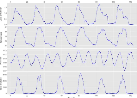
bees on average, per day. Figure 2 shows a section of the data employed in this research, where the time series of activity level and weather can be observed.
The Model.
Multi-layer Perceptron Artificial Neural Networks are a machine learning method engineered as an analogy to the brain’s behavior29,30. Simple processing units, called neurons, linked in a network, arerespon-sible for calculating mathematical functions that allow fitting inputs to outputs31. Depending on the problem we
want to solve, different architectures (or topologies) can be exploited in the search for the best fit. Linearly sepa-rable problems often can be solved with one layer of neurons, however, non-linear problems usually need more layers to be able to perform best fits. Neural Networks have been applied in many contexts, such as forecasting of drylands32, classification of human electroencephalogram33, monitoring of memory34, robotics and computer
vision35.
Recurrent Neural Networks extends regular Neural Networks by adding the capability of recurrences within the neurons. This recurrence allows the network to handle variable-length sequences36. In doing so, the Recurrent
Neural Networks present the ability to store internal memory and to deal more naturally with dynamic temporal behavior37–39. In its usual form, the recurrence is represented by h( )t =f h( ( 1)t− ,x( )t; )θ, where h is the hidden state
at time t. ht( 1)− represents the previous hidden state. xt() is the current input vector and θ is the set of shared
parameters through time. As mentioned by Gomes et al.8, originally, RNNs were difficult to train due to the
prob-lem of the vanishing gradient. It is also mentioned in the work by Chung et al.20. Huang et al.40 describe this
phenomenon in the following way: “as the gradient information is back-propagated, repeated multiplication with small weights renders the gradient information ineffectively small in earlier layers”. Hence, to overcome this prob-lem, some methods have been proposed, as the clipped gradient presented by Chung and colleagues20 and the use
of activation function with gated units. Gated units are able to monitor the quantity of data that enters the unit, the quantity of data that is stored and the quantity of data that is forwarded to the next units. The two more effec-tive types of gated unit are the Long Short-Term Memory (LSTM)7 and the Gated Recurrent Units (GRU)6.
For the RNN deployment, we use Keras (https://keras.io) with Theano (http://deeplearning.net/software/ theano) backend. Scikit-Learn (https://scikit-learn.org/stable) was also used to allow getting metrics and methods for normalization. The RNN was built on Python 3.7.
Exploiting RNN Topologies.
In order to find the most suitable RNN topology to forecast the activity level of bees, we initially investigate eight different recurrent neural networks, considering four topologies (with differ-ent number of neurons and layers) and differdiffer-ent gated units (GRU and LSTM). The designed topologies were built with: two hidden layers with two recurrent units in each layer (2X2), two hidden layers with five recurrent units in each layer (2x5), five hidden layers with two recurrent units each (5x2), and five hidden layers with five recurrent Figure 1. The system environment. (a) The eight M. fasciculata hives employed in this study. (b) Frontal view of the adapted hive entrance: it contains a PVC box for storing electronic items. (c) Electronic system details: (1) Intel Edison TM for RFID reader control and data storage, (2) USB RFID reader, (3) Transparent hose where the bees pass upon the RFID reader, (4) Hive of M. fasciculata, and (5) PVC box. (d) Tagged M. fasciculata at the hive entrance.units in each layer (5x5). Hence, the eight models designed to the investigation are: {GRU2x2, GRU2x5, GRU5x2, GRU5x5} and {LSTM2x2, LSTM2x5, LSTM5x2, LSTM5x5}. Figure 3 depicts one of the proposed architectures (specifically 2x2).
Related to training and testing each architecture, we employ a hold-out method. We evaluate the model using the Root Mean Square Error (RMSE), which is obtained by:
∑
= − = ˆ RMSE n y y 1 ( ) i n i i 1 2where y is the observed value and ˆy is the predicted value by the model.
In the hold-out method, the datasets are randomized, and usually, 2/3 of the data is used for the training of the model, and the remaining 1/3 is used for the model evaluation. In our study, each model was trained and evaluated 30 times, allowing a more confident statistical evaluation. The initial evaluation aimed to determine the most suitable RNN topology for our data. The data were organized into a table consisting of 5 columns, the first four being the RNN inputs (temperature, barometric pressure, solar irradiance, previous activity), and the fifth the expected output in hours’ time (see Fig. 3).
Figure 2. Section of the time series employed in this research, from August 7th to 12th, 2015. It presents hourly values of bees’ level of activity, temperature (°C), barometric pressure (hPa) and solar irradiance (kJ/m2).
Figure 3. One of the developed topologies: it consists of 4 neurons organized in two hidden layers. In this figure, we show as inputs: Activity Level, Temperature, Solar Irradiance and Barometric Pressure. The output is the forecast of Activity Level at t + 1. Evaluated hidden layers are LSTM and GRU.
As previously mentioned, as a first step we seek to exploit several RNN architectures. After that, we evaluate how different input size windows impact on the accuracy of the forecast. Finally, we show how algorithms of attribute selection and correlation analysis can help in improving even further the accuracy of the forecast.
Finding the Best Size for the Input Window.
Aiming to advance the results of the forecast, a second evaluation was performed. We employ the best architecture found in the previous step and evaluate different sizes for the input window, that is, different amounts of preceding data to forecast the next level. It demands the RNN the ability to keep valuable information through time. The evaluations were undertaken to employ the current hour, 3, 6, 12, 24, 36, 48, and 60 hours prior to the event.Henceforth, we represent current hour as t0 and 3, 6, 12, 24, 36, 48 and 60 hours as t−2, t−5, t−11, t−23, t−35, t−47,
t−59 (see Table 1 and Fig. 4). We perform the same test using bees’ level of activity and environmental variables
(solar irradiance, barometric pressure and temperature). Table 1 shows the evaluated input vectors (for bees’ level of activity, barometric pressure, solar irradiance and temperature).
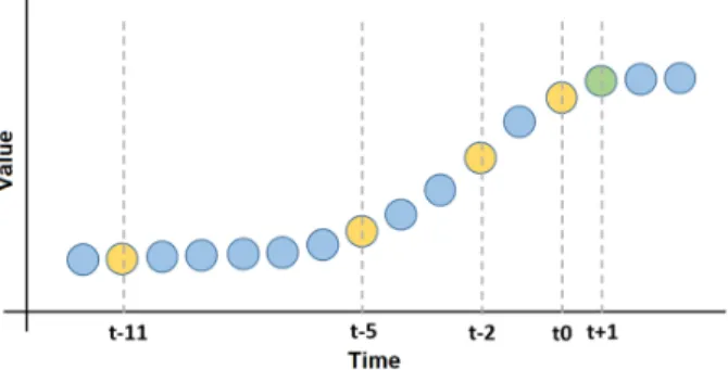
Figure 4 presents a schematic diagram presenting generic inputs and outputs values to be used in the forecast model. The figure presents the model we use, although, it does not represent real data gathered by the system. The aim is intended to graphically represent the mean in winch the values are employed. In this figure, we represent the window w12 which is a vector composed by the current time (t0), 3, 6 and 12 hours prior the event to forecast.
Selecting the Best Environmental Features.
Our third effort to improve the forecast accuracy was per-formed using a technique to select the best environmental predictors. This process consists of selecting the best time window for each variable, join them in one dataset and select the most important ones with lower temporal correlation. As Table 1 shows, each window can have a maximum of 8 temporal values. It means that, a dataset incorporating all 3 environmental variables could have 24 features. For this reason, we selected the best features based on feature importance score and correlation values.In order to calculate the feature importance score, we used the Permutation Feature Importance (PFI) method. This algorithm works as shown in Fig. 5. After it shuffles a variable, it allows the verification of the new value of RMSE, guiding the process of removing unnecessary or disturbing features. The PFI works by fitting the RNN with the training set and then applying this RNN to the test data (Dt). The RMSE found is called Eo. Each input feature is shuffled on the corresponding column Dt generating Dt′. Applying the RNN on this Dt′ will give us a new RMSE called Ed. The difference between Ed and Eo is called the feature importance score of the “suffled” feature. A high score means that Ed is bigger than Eo, in other words, removing the particular feature increases the model’s RMSE.
Reference Used Values (Input Vector) Forecast
w1 t0 t+1 w3 t0, t−2 t+1 w6 t0, t−2, t−5 t+1 w12 t0, t−2, t−5, t−11 t+1 w24 t0, t−2, t−5, t−11, t−23 t+1 w36 t0, t−2, t−5, t−11, t−23, t−35 t+1 w48 t0, t−2, t−5, t−11, t−23, t−35, t−47 t+1 w60 t0, t−2, t−5, t−11, t−23, t−35, t−47, t−59 t+1
Table 1. Structure of the evaluated input vectors (for bees’ level of activity, barometric pressure, solar irradiance and temperature). Related to the input vector, t0 means the current time (i.e. the hour before the event to
forecast), t−2 means 3 hours before the event to forecast, t−5 means 6 hours before the event to forecast an so on.
Figure 4 shows a graphical representation of the input vector.
Figure 4. Schematic diagram presenting generic inputs and outputs values to be used in the forecast model. The points in orange represent the values to be employed as inputs of the RNN. The points in green represent output values. Note that this is a generic time series and it is not intended to directly represent real data.
Results
Investigation on RNN architectures.
Our first evaluation aims to understand which is the best topology to solve our forecast problem. We take into account the current level of activity (actt0) and environmental featuressuch as temperature (tempt0), solar irradiance (radt0), and barometric pressure (presst0) to forecast the next level
of activity (actt+1). Due to the random initialization of the network’s weights, each architecture was trained and
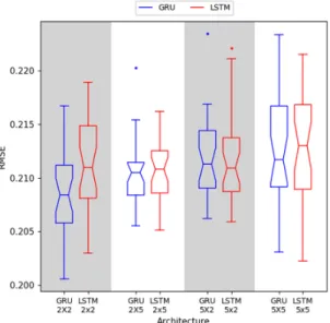
evaluated 30 times. Figure 6 presents the error (RMSE) for each architecture.
In order to validate which RNN architecture best suited this context, the 8 RNNs were statistically compared. First, we used the Shapiro-Wilk normality test to verify the distribution of the results. For all the sets, except GRU2x5, the Shapiro-Wilk showed p-values larger than 0.05, which means that the distributions can be accepted as parametric ones (i.e. Gaussian distributions). Hence, we employed the Welch Two Sample t-test to determine the similarity among the results. Since the GRU2x2 showed the lowest median (RMSE = 0.208), we compared it to the others. The comparison of GRU2x2 (lowest median) with other architectures showed p-values smaller than 0.05. Thus, GRU2x2 is the most appropriate architecture for the proposed context.
Investigation on the input window size of bees’ level of activity and weather attributes.
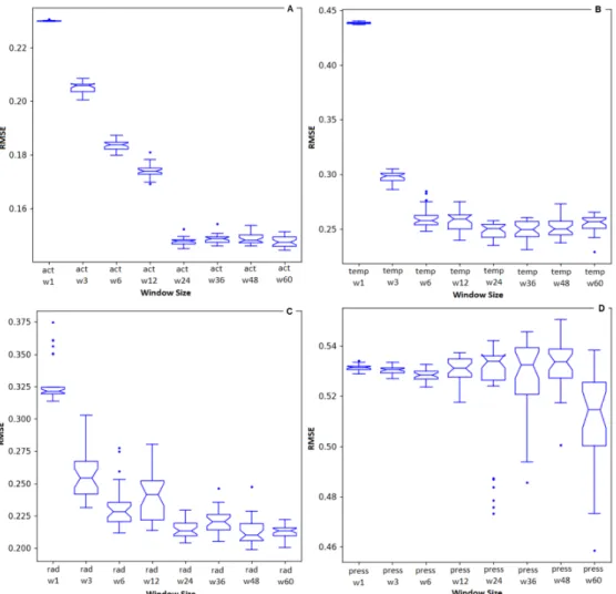
Our second evaluation aims to determine the best size for the input window. Input attributes were analyzed individ-ually in order to find the best temporal window size for each one. Hence, we employed the best topology found in the previous evaluation with different windows size (input vectors w1 to w60, as shown in Table 1). We took into account the following inputs: bees’ level of activity, temperature, solar irradiance and barometric pressure.Figure 7 shows the errors for each different input vector. Results are presented from 30 executions of each RNN. Figure 7(a) shows the error taking into account different window size of preceding level of activity fore-casting next levels of activity. The best (lowest) median value was found in the set Actw60 with an RMSE of 0.147.
We performed a statistical test among the sets to verify if any other set is equivalent to the Actw60. The Welch Two
Sample t-test between Actw60 and Actw24 showed a p-value of 0.90. Hence, the sets can be considered as equivalent
with a confidence level of 95%. Taking into account that the set Actw24 used fewer variables and the results were
statistically equivalent to Actw60, we chose Actw24 as the best set of attributes level of activity forecasting next levels
of activity.
Figure 7(b) shows the error taking into account different window size of temperature forecasting levels of activity. The best (lowest) median value was found in the set Tempw36 with an RMSE of 0.249. We performed
Figure 5. Feature Importance algorithm.
Figure 6. Result (RMSE) for each architecture. A Welch Two Sample t-test showed that the GRU2x2 RNN outperforms the other topologies. The GRU2x2 RNN shows a mean RMSE of 0.208.
a statistical test among the sets to verify if any other set was equivalent to the Tempw36. The Welch Two Sample
t-test between Tempw36 and Tempw24 showed a p-value of 0.60. Hence, the sets can be considered as equivalent
with a confidence level of 95%. Taking into account that the set Tempw24 used fewer variables and that the results
were statistically equivalent to Tempw36, we chose Tempw24 as the best set for the attribute temperature forecasting
next levels of activity. Figure 7(c) shows the error taking into account different window size of solar irradiance forecasting levels of activity. The best (lowest) median valeu was found in the set Radw48 with an RMSE of 0.210.
We performed a statistical test among the sets to verify if any other set was equivalent to the Radw48. The Welch
Two Sample t-test between Radw48 and Radw24 showed a p-value of 0.52. Hence, the sets can be considered as
equivalent with a confidence level of 95%. Taking into account that the set Radw24 used fewer variables and that
the results were statistically equivalent to Radw48, we chose Radw24 as the best set for the attribute solar irradiance
forecasting levels of activity.
Finally, Fig. 7(d) shows the error taking into account different window size of barometric pressure forecasting levels of activity. The best (lowest) median was found in the set Pressw60 with an RMSE of 0.514. We performed a
statistical test among the sets to verify if any other set was equivalent to the Pressw60. No other set showed
statis-tical similarity, being all the comparisons presenting p-values lower than 0.05. Hence, the sets can be considered distinct with a confidence level of 95%. Taking into account that the set Radw60 showed the best median value and
no other set was equivalent, we chose Pressw60 as the best set for the attribute barometric pressure forecasting levels
of activity.
The next section presents a combination of the best sets of activity and weather variables obtained in this evaluation, seeking to improve accuracy.
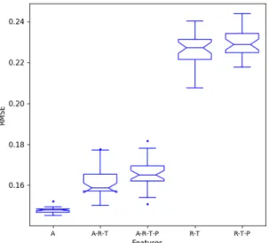
Combining Features. After determining the best window size for each attribute, we extended the analysis by test-ing various combinations of attribute predictors. Thus, the followtest-ing sets were created: {Activity (A)}, {Activity, Solar Irradiance, Temperature (ART)}, {Activity, Solar Irradiance, Temperature, Barometric Pressure (ARTP)}, {Solar Irradiance, Temperature (RT)}, {Solar Irradiance, Temperature, Barometric Pressure (RTP)}.
Figure 7. RMSE for each evaluated window size. (a) Activity. (b) Temperature. (c) Solar Irradiance. (d) Barometric Pressure.
For theses sets, we employed the best input size windows found in the previous evaluation: activity, solar irradiance and temperature using window = 24 and barometric pressure using window = 60. We evaluate sets with both previous activity (sets with A) or not (sets without A), since the data from activity may not always be available – in this case, we can estimate the level of activity using weather variables alone. The main motivation in using environmental variables to forecast bees’ activities is motivated by the fact that the RFID system is not always available for use due to the cost and/or management aspects.
Figure 8 shows the result (RMSE) for the feature combination with the best windows size of each attribute. We can see that using previous activity (w24) alone is the best to forecast next levels. Although it seems that the sets in which barometric pressure is used, have decreased accuracy, a statistical comparison among RT and RTP shows that they are statistically equivalent.
As previously defined, the activity level is calculated considering the total number of bees’ activities divided by the number of live bees at that period. Which means that, knowing the activity levels of the preceding 24 hours, we can forecast the level of activity with an average RMSE of 0.147. Since the activity level ranged from 0.0 to 2.0, the mean error of this configuration is about 8%. Taking into account that the average error in the first evaluation (GRU2x2 ARTP_w1) was 0.208 and the average error using the ACT_w24 is 0.147, we have about 30% improve-ment in the accuracy by using ACT_w24 window size as input.
In the next section we exploit the Permutation Feature Importance algorithm and perform a Correlation Analysis aiming to improve the forecast accuracy, employing weather variables alone.
Feature importance and correlation analisys.
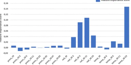
We aim to investigate the importance of environmen-tal variables alone as the predictors for bees’ activity level, employing the following environmenenvironmen-tal variables: solar irradiance (R), temperature (T) and barometric pressure (P). Therefore, we exploit the Permutation Feature Importance algorithm and perform a Correlation Analysis. We took into account the best sets found in previous section: Solar Irradiance and Temperature with w24 and Barometric Pressure with w60.Figure 9 shows the feature importance score for each attribute. We can see that temperature and solar irradi-ance present higher scores, which suggests a strong influence on bees’ activity level. Furthermore, we can see some attributes with lower than zero score, which suggests that they are decreasing model’s accuracy. Figure 10 shows the feature correlation heatmap. Highly correlated attributes are often considered redundant because they do not add useful information to the model. Furthermore, they can add noise and be a confounding factor in the training of models. Hence it is a good practice to remove highly correlated attributes.
We created 3 new datasets based on the results of feature importance (scores) and correlation values. The first considers all features with score larger than 0.0 (named FSL0). We then evaluated the correlation among the attributes, and created datasets removing attributes that showed correlation larger than 70% and 80% (named CORR70 and CORR80 [upon FSL0]). We aim to evaluate if the accuracy improves when removing highly corre-lated attributes, given that highly correcorre-lated attributes may be a confounding factor when used in conjunction.
Figure 11 shows the result of the RNN when using sets with feature score larger than 0 (FSL0), sets removing correlated attributes (correlation greater than 80% and 70%), and also shows the RTP found in the evaluation of window size (R_w24, T_w24, P_w60). We used the Shapiro-Wilk normality test to verify the adequacy of the results to parametric or non-parametric distributions. For all the sets the Shapiro-Wilk showed p-values larger than 0.05, which means that the distributions can be accepted as parametric ones. Hence, we employed the Welch Two Sample t-test to verify the similarity among the results. The comparison showed that both sets are distinct from each other, since all tests showed p-value smaller than 0.05 – It means that the results are statistically distinct with 95% of confidence. The best one is the CORR80 since it showed the lowest error.
We can see that the PFI outperforms the regular RTP since it can remove features that have a confounding effect upon model’s accuracy. Moreover, we can see that the mapping results of correlation analysis also Figure 8. Result (RMSE) for the feature combination incorporating the best window size for each attribute.
demonstrated that a correlation threshold of 80% was ideal in our experiment, however, it must be highlighted that this value is likely problem dependent.
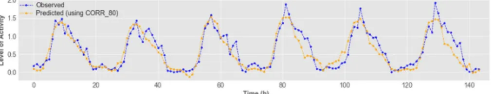
Employing weather variables alone, and using a technique to find the best window size, allowed us to obtain an average RMSE error of 0.229 (Section “Investigation on the Input Window Size of Bees’ Level of Activity and Weather Attributes”). After employing the PFI and performing an analysis of correlated variables, we were able to decrease the average RMSE error to 0.212, being approximately 7.5% better. Figure 12 shows a subset of six days of our data, presenting observed and predicted values, using environmental attributes as predictors.
Conclusion and Future Work
This work aimed to investigate RNN on the task of predicting bees’ level of activity, which can be approached as a time-series forecasting problem. In the first step, we investigated eight different RNN upon data from bees’ activity and environmental data (temperature, solar irradiance and barometric pressure) finding that GRU out-performs LSTM in this particular problem. It was followed by the evaluation of the best window size for each attribute, in which we perceive that employing larger inputs help improving the accuracy of the model. For exam-ple, knowing the activity levels of the preceding 24 hours allowed us to forecast the level of activity with an average RMSE of 0.147, being about 30% better than using only one hour ahead attributes.
In the final step, we exploited the Permutation Feature Importance algorithm and performed a Correlation Analysis aiming to improve the forecast accuracy employing environmental variables alone. Based on the assumption mentioned before, the cost and/or technical aspects could make the RFID system unavailable. For Figure 9. Feature Importance score for each attribute. Higher the score, higher the influence to improve model’s accuracy.
this reason, we investigated the importance of as predictors for bees’ activity level, employing the following envi-ronmental variables: solar irradiance (R), temperature (T) and barometric pressure (P). Employing weather var-iables alone, and using a technique to find the best window size, allowed us to obtain an average RMSE error of 0.229. After employing the PFI and an analysis of correlated variables, we were able to decrease the average RMSE error to 0.212, being approximately 7.5% better.
A better understanding of bees’ behavior can contribute to the environment, fruit producers and to our lives. In this research, we pointed out a way to improve forecast of bees’ activity by means of RNNs. Although, there are some future work we plan to tackle in the continuity of this project; those are more related to the environmental evaluation and the influence of (i) parasites, (ii) pesticides, (iii) weather changes, (iv) monoculture farming, and (v) inappropriate management of beehives.
Data availability
The data we use in this study is available at https://doi.org/10.13140/RG.2.2.14287.02723. A sample source-code can be found at https://doi.org/10.13140/RG.2.2.27938.17603.
Received: 10 May 2019; Accepted: 7 December 2019; Published: xx xx xxxx
References
1. Potts, S. G. et al. Safeguarding pollinators and their values to human well-being. Nature 540, 220–229 (2016).
2. Nunes-Silva, P., Hrncir, M., da Silva, C. I., Roldão, Y. S. & Imperatriz-Fonseca, V. L. Stingless bees, melipona fasciculata, as efficient pollinators of eggplant (solanum melongena) in greenhouses. Apidologie 44, 537–546 (2013).
3. Nunes-Silva, P. et al. Applications of rfid technology on the study of bees. Insectes sociaux 66, 15–24 (2019).
4. Potts, G. et al. Global pollinator declines: Trends, impacts and drivers. Trends in Ecology and Evolution 25, 345–353 (2010). 5. Ratnieks, F. L. W. & Carreck, N. L. Clarity on honey bee collapse? Science (New York, N.Y.) 327, 152–3 (2010).
6. Bahdanau, D., Cho, K. & Bengio, Y. Neural machine translation by jointly learning to align and translate. arXiv preprint arXiv:1409.0473 (2014).
7. Hochreiter, S. & Schmidhuber, J. Long short-term memory. Neural computation 9, 1735–1780 (1997).
8. Gomes, P. A. B., de Carvalho, E. C., Arruda, H., Souza, P. & Pessin, G. Exploiting recurrent neural networks in the forecasting of bees’ level of activity. In The 26th International Conference on Artificial Neural Networks (ICANN), 1–8 (2017).
9. Schultz, K. M., Passino, K. M. & Seeley, T. D. The mechanism of flight guidance in honeybee swarms: subtle guides or streaker bees? Journal of Experimental Biology 211, 3287–3295 (2008).
Figure 11. Results using sets with feature score larger than 0 (FSL0), sets removing correlated attributes (correlation greater than 80% and 70%) and sets with the best window size of RTP found in previous section (R_w24, T_w24, P_w60).
Figure 12. Observed and predicted activity levels, using attributes with lower than 80% correlation and higher than zero permutation feature importance score.
10. Schwager, M., Anderson, D. M., Butler, Z. & Rus, D. Robust classification of animal tracking data. Computers and Electronics in Agriculture 56(2007), 46–59 (2006).
11. Schaerf, T. M., Dillingham, P. W. & Ward, A. J. The effects of external cues on individual and collective behavior of shoaling fish. Science advances 3, e1603201 (2017).
12. Chena, C., Yangb, E.-C., Jianga, J.-A. & Lina, T.-T. An imaging system for monitoring the in-and-out activity of honey bees. Computers and Electronics in Agriculture 89, 100–109 (2012).
13. Tu, G. J., Hansen, M. K., Kryger, P. & Ahrendt, P. Automatic behaviour analysis system for honeybees using computer vision. Computers and Electronics in Agriculture 122, 10–18 (2016).
14. Gil-Lebrero, S. et al. Honey bee colonies remote monitoring system. Sensors 17, 55 (2017).
15. Arruda, H., Imperatriz-Fonseca, V., de Souza, P. & Pessin, G. Identifying bee species by means of the foraging pattern using machine learning. In 2018 International Joint Conference on Neural Networks (IJCNN), 1–6 (IEEE, 2018).
16. Gama, F., Arruda, H., Carvalho, H. V., de Souza, P. & Pessin, G. Understanding of the behavior of bees through anomaly detection techniques. In The 26th International Conference on Artificial Neural Networks (ICANN), 1–8 (2017).
17. Ho, T. K. Random decision forests. In Proceedings of the Third International Conference on Document Analysis and Recognition (Volume 1) - Volume 1, ICDAR ’95, 278– (IEEE Computer Society, Washington, DC, USA, 1995).
18. Breunig, M. M., Kriegel, H.-P., Ng, R. T. & Sander, J. Lof: Identifying density-based local outliers. SIGMOD Rec. 29, 93–104, https:// doi.org/10.1145/335191.335388 (2000).
19. Martens, J. & Sutskever, I. Learning recurrent neural networks with hessian-free optimization. International Conference on Machine Learning, Bellevue, WA, USA 28 (2011).
20. Chung, J., Gulcehre, C., Cho, K. & Bengio, Y. Empirical evaluation of gated recurrent neural networks on sequence modeling. NIPS 2014 Deep Learning and Representation Learning Workshop (2014).
21. Jozefowicz, R., Zaremba, W. & Sutskever, I. An empirical exploration of recurrent network architectures. Journal of Machine Learning Research 37, 2342–2350 (2015).
22. de Carvalho, E. C. et al. Exploiting the use of recurrent neural networks for driver behavior profiling. In 2017 International Joint Conference on Neural Networks (IJCNN), 3016–3021, https://doi.org/10.1109/IJCNN.2017.7966230 (2017).
23. Karpathy, A., Johnson, J. & Li, F. Visualizing and understanding recurrent networks. CoRR abs/1506.02078 (2015).
24. Britz, D., Goldie, A., Luong, M. & Le, Q. V. Massive exploration of neural machine translation architectures. CoRR abs/1703.03906 (2017).
25. Altmann, A., Toloşi, L., Sander, O. & Lengauer, T. Permutation importance: a corrected feature importance measure. Bioinformatics
26, 1340–1347 (2010).
26. Breiman, L. Random forests. Machine Learning 45, 5–32, https://doi.org/10.1023/A:1010933404324 (2001).
27. Suhara, Y., Xu, Y. & Pentland, A. Deepmood: Forecasting depressed mood based on self-reported histories via recurrent neural networks. In Proceedings of the 26th International Conference on World Wide Web, 715–724, https://doi.org/10.1145/3038912.3052676
(2017).
28. De Souza, P. et al. Low-cost electronic tagging system for bee monitoring. Sensors 18, https://doi.org/10.3390/s18072124 (2018). 29. Haykin, S. Neural networks and learning machines, vol. 3 (Pearson Upper Saddle River, NJ, 2009).
30. Bayat, F. M. et al. Implementation of multilayer perceptron network with highly uniform passive memristive crossbar circuits. Nature communications 9, 2331 (2018).
31. Szczuka, M. & Ślęzak, D. Feedforward neural networks for compound signals. Theoretical Computer Science 412, 5960–5973 (2011). 32. Buckland, C., Bailey, R. & Thomas, D. Using artificial neural networks to predict future dryland responses to human and climate
disturbances. Scientific reports 9, 3855 (2019).
33. Nejedly, P. et al. Exploiting graphoelements and convolutional neural networks with long short term memory for classification of the human electroencephalogram. Scientific reports 9, 1–9 (2019).
34. Zakrzewski, A. C., Wisniewski, M. G., Williams, H. L. & Berry, J. M. Artificial neural networks reveal individual differences in metacognitive monitoring of memory. PloS one 14, e0220526 (2019).
35. Ondruska, P. & Posner, I. Deep tracking: Seeing beyond seeing using recurrent neural networks. In Thirtieth AAAI Conference on Artificial Intelligence (2016).
36. Goodfellow, I., Bengio, Y. & Courville, A. Deep Learning, http://www.deeplearningbook.org (MIT Press, 2016). 37. Yu, D. & Deng, L. Automatic speech recognition: A deep learning approach (Springer, 2014).
38. LeCun, Y., Bengio, Y. & Hinton, G. Deep learning. Nature 521, 436–444 (2015).
39. Tsironi, E., Barros, P., Weber, C. & Wermter, S. An analysis of convolutional long short-term memory recurrent neural networks for gesture recognition. Neurocomputing 268, 76–86, https://doi.org/10.1016/j.neucom.2016.12.088 (2017).
40. Huang, G., Sun, Y., Liu, Z., Sedra, D. & Weinberger, K. Q. Deep networks with stochastic depth. In European conference on computer vision, 646–661 (Springer, 2016).
Acknowledgements
Pedro A.B. Gomes would like to acknowledge the Capes Foundation, Ministry of Education of Brazil, due to his scholarship. Prof. Vera Lucia Imperatriz-Fonseca acknowledge MCTIC/CNPq-Brazil process 312250/2018-5. Dr. Gustavo Pessin acknowledge MCTIC/CNPq-Brazil process 429096/2018-6.
Author contributions
Conceptualization: P.G., Y.S., P.N.S., V.F., A.P., P.d.S. and G.P.; Field methodology: P.N.S., G.V., V.F., P.d.S. and G.P.; Field dataset collection: P.N.S., L.C., H.A., G.V., V.F., P.d.S. and G.P.; Field dataset curation: G.P.; Machine-learning methodology: P.G., Y.S., A.P. and G.P.; Machine-learning development: P.G.; Conceived images and graphics: P.G., L.C., H.A. and G.P.; Analysed the results: P.G., Y.S., P.N.S., V.F., A.P., P.d.S. and G.P.; Write the manuscript: P.G., Y.S., P.N.S., H.A., G.V., V.F., A.P., P.d.S. and G.P. All authors reviewed the manuscript.
Competing interests
The authors declare no competing interests.
Additional information
Correspondence and requests for materials should be addressed to G.P. Reprints and permissions information is available at www.nature.com/reprints.
Publisher’s note Springer Nature remains neutral with regard to jurisdictional claims in published maps and institutional affiliations.