CBMM Memo No. 047
April 12, 2016
Bridging the Gaps Between Residual Learning,
Recurrent Neural Networks and Visual Cortex
by
Qianli Liao and Tomaso Poggio
Center for Brains, Minds and Machines, McGovern Institute, MIT
Abstract:
We discuss relations between Residual Networks (ResNet), Recurrent Neural Networks (RNNs) and the primate visual cortex. We begin with the observation that a shallow RNN is exactly equivalent to a very deep ResNet with weight sharing among the layers. A direct implementation of such a RNN, although having orders of magnitude fewer parameters, leads to a performance similar to the corresponding ResNet. We propose 1) a generalization of both RNN and ResNet architectures and 2) the conjecture that a class of moderately deep RNNs is a biologically-plausible model of the ventral stream in visual cortex. We demonstrate the effectiveness of the architectures by testing them on the CIFAR-10 dataset.This work was supported by the Center for Brains, Minds and Machines
(CBMM), funded by NSF STC award CCF - 1231216.
1
Introduction
Residual learning [8], a novel deep learning scheme characterized by ultra-deep architectures has recently achieved state-of-the-art performance on several popular vision benchmarks. The most recent incarnation of this idea [10] with hundreds of layers demonstrate consistent performance improvement over shallower networks. The 3.57% top-5 error achieved by residual networks on the ImageNet test set arguably rivals human performance.
Because of recent claims [33] that networks of the AlexNet[16] type successfully predict properties of neurons in visual cortex, one natural question arises: how similar is an ultra-deep residual network to the primate cortex? A notable difference is the depth. While a residual network has as many as 1202 layers[8], biological systems seem to have two orders of magnitude less, if we make the customary assumption that a layer in the NN architecture corresponds to a cortical area. In fact, there are about half a dozen areas in the ventral stream of visual cortex from the retina to the Inferior Temporal cortex. Notice that it takes in the order of 10ms for neural activity to propagate from one area to another one (remember that spiking activity of cortical neurons is usually well below 100 Hz). The evolutionary advantage of having fewer layers is apparent: it supports rapid (100msec from image onset to meaningful information in IT neural population) visual recognition, which is a key ability of human and non-human primates [31, 28].
It is intriguingly possible to account for this discrepancy by taking into account recurrent connections within each visual area. Areas in visual cortex comprise six different layers with lateral and feedback connections [17], which are believed to mediate some attentional effects [2, 17, 14, 25, 12] and even learning (such as backpropagation [20]). “Unrolling” in time the recurrent computations carried out by the visual cortex provides an equivalent “ultra-deep” feedforward network, which might represent a more appropriate comparison with the state-of-the-art computer vision models.
In addition, we conjecture that the effectiveness of recent “ultra-deep” neural networks primarily come from the fact they can efficiently model the recurrent computations that are required by the recognition task. We show compelling evidences for this conjecture by demonstrating that 1. a deep residual network is formally equivalent to a shallow RNN; 2. such a RNN with weight sharing, thus with orders of magnitude less parameters (depending on the unrolling depth), can retain most of the performance of the corresponding deep residual network.
Furthermore, we generalize such a RNN into a class of models that are more biologically-plausible models of cortex and show their effectiveness on CIFAR-10.
2
Equivalence of ResNet and RNN
2.1
Intuition
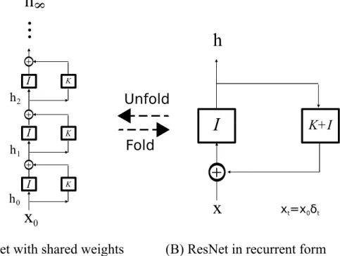
We discuss here a very simple observation: a Residual Network (ResNet) approximates a specific, standard Recurrent Neural Network (RNN) implementing the discrete dynamical system described by
ht= K ◦ (ht−1) + ht−1 (1)
where ht is the activity of the neural layer at time t and K is a nonlinear operator. Such a dynamical systems corresponds to the feedback system of Figure 1 (B). Figure 1 (A) shows that unrolling in (discrete) time the feedback system gives a deep residual network with the same (that is, shared) weights among the layers. The number of layers in the unrolled network corresponds to the discrete time iterations of the dynamical system. The identity shortcut mapping that characterizes residual learning appears in the figure.
Thus, ResNets with shared weights can be reformulated into the form of a recurrent system. In section 5.2) we show experimentally that a ResNet with shared weights retains most of its performance (on CIFAR-10).
K K K
I
I
I
I
+
h
x
x
0h
+ + +...
(A) ResNet with shared weights (B) ResNet in recurrent form
K+I
8
h
0h
1h
2x
t=x
0δ
tFold
Unfold
Figure 1: A formal equivalence of a ResNet (A) with weight sharing and a RNN (B). I is the identity operator. K is an operator denoting the nonlinear transformation called f in the main text. xtis the value of the input at time t. δtis a Kronecker delta function.
2.2
Formulation in terms of Dynamical Systems (and Feedback)
We frame recurrent and residual neural networks in the language of dynamical systems. We consider here dynamical systems in discrete time, though most of the definitions carry over to continuous time. A neural network (that we assume for simplicity to have a single layer with n neurons) can be a dynamical system with a dynamics defined as
ht+1= f (ht; wt) + xt (2)
where ht∈ Rn is the activity of the n neurons in the layer at time t and f : Rn → Rn is a continuous, bounded function parametrized by the vector of weights wt. In a typical neural network, f is synthesized by the following relation between the activity yt of a single neuron and its inputs xt−1:
yt= σ(hw, xt−1i + b), (3)
where σ is a nonlinear function such as the linear rectifier σ(·) = | · |+.
A standard classification of dynamical systems defines the system as
1. homogeneous if xt= 0, ∀t > 0 (alternatively the equation reads as ht+1= f (ht; wt) with the inital condition h0= x0)
2. time invariant if wt= w.
Residual networks with weight sharing thus correspond to homogeneous, time-invariant systems which in turn correspond to a feedback system (see Figure 1) with an input which is non-zero only at time t = 0 (xt=0= x0, xt= 0 ∀t > 0) and with f (z) = (K + I) ◦ z:
hn = f (ht; wt) = (K + I)n◦ x0 (4) “Normal” residual networks correspond to homogeneous, time-variant systems. An analysis of the corresponding inhomogeneous, time-invariant system is provided in the Appendix.
3
A Generalized RNN for Multi-stage Fully Recurrent Processing
As shown in the previous section, the recurrent form of a ResNet is actually shallow (if we ignore the possible depth of the operator K). In this section, we generalize it into a moderately deep RNN that reflects the multi-stage processing in the primate visual cortex.
3.1
Multi-state Graph
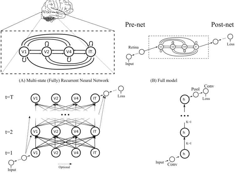
We propose a general formulation that can capture the computations performed by a multi-stage processing hierarchy with full recurrent connections. Such a hierarchy can be characterized by a directed (cyclic) graph G with vertices V and edges E.
G = {V, E} (5)
where vertices V is a set contains all the processing stages (i.e., we also call them states). Take the ventral stream of visual cortex for example, V = {LGN, V 1, V 2, V 4, IT }. Note that retina is not listed since there is no known feedback from primate cortex to the retina. The edges E are a set that contains all the connections (i.e., transition functions) between all vertices/states, e.g., V1-V2, V1-V4, V2-IT, etc. One example of such a graph is in Figure 2 (A).
3.2
Pre-net and Post-net
The multi-state fully recurrent system does not have to receive raw inputs. Rather, a (deep) neural network can serve as a preprocesser. We call the preprocesser a “pre-net” as shown in Figure 2 (B). On the other hand, one also needs a “post-net” as a postprocessor and provide supervisory signals to the recurrent system and the pre-net. The pre-net, recurrent system and post-net are trained in an end-to-end fashion with backpropagation.
For most models in this paper, unless stated otherwise, the pre-net is a simple 3x3 convolutional layer and the post-net is a pipeline of a batch normalization, a ReLU, a global average pooling and a fully connected layer (or a 1x1 convolution, we use these terms interchangeably).
Take primate visual system for instance, the retina is a part of the “pre-net”. It does not receive any feedback from the cortex and thus can be separated from the recurrent system for simplicity. In Section 5.3.3, we also tried 3 layers of 3x3 convolutions as an pre-net, which might be more similar to a retina, and observed slightly better performance.
3.3
Transition Matrix
The set of edges E can be represented as a 2-D matrix where each element (i,j) represents the transition function from state i to state j.
One can also extend the representation of E to a 3-D matrix, where the third dimension is time and each element (i,j,t) represents the transition function from state i to state j at time t. In this formulation, the transition functions
V1 V2 V4 IT
(A) Multi-state (Fully) Recurrent Neural Network (B) Full model
V1 V2 V4 IT
Pre-net Post-net
Input Retina Loss ... ...(C) Simulating our model in time by unrolling (D) An example ResNet: for comparison
V1 V2 V4 IT
t=T
t=2
t=1
V1 V2 V4 IT V1 V2 V4 IT...
Loss ... Input ... h h h Loss Input Conv Pool Conv K+I K+I...
OptionalFigure 2: Modeling the ventral stream of visual cortex using a multi-state fully recurrent neural network
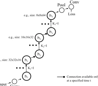
can vary over time (e.g., being blocked from time t1 to time t2, etc.). The increased expressive power of this formulation allows us to design a system where multiple locally recurrent systems are connected sequentially: a downstream recurrent system only receives inputs when its upstream recurrent system finishes, similar to recurrent convolutional neural networks (e.g., [19]). This system with non-shared weights can also represent exactly the state-of-the-art ResNet (see Figure 3).
Nevertheless, time-dependent dynamical systems, that is recurrent networks of real neurons and synapses, offer interesting questions about the flexibility in controlling their time dependent parameters.
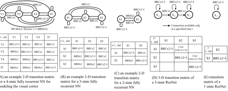
Example transition matrices used in this paper are shown in Figure 4.
When there are multiple transition functions to a state, their outputs are summed together.
3.4
Shared vs. Non-shared Weights
Weight sharing is described at the level of an unrolled network. Thus, it is possible to have unshared weights with a 2D transition matrix — even if the transitions are stable over time, their weights could be time-variant.
h h h Loss Input Conv Pool Conv K+I K+I
...
(A) ResNet without changing spacial&feature sizes (B) ResNet with changes of spacial&feature sizes (He et. al.)
h h Loss Input Conv Pool Conv K1+I e.g., size: 32x32x16 e.g., size: 32x32x16 e.g., size: 32x32x16 h h K2+I h h K3+I
...
...
...
e.g., size: 16x16x32 e.g., size: 8x8x64(C) Recurrent form of A (D) Recurrent form of B
h
Pre-net
Post-net
h h h Subsample &increase features Subsample &increase features 2 1 1 2 3 3 3 2 1Connection available only at a specified time t
Post-net
Pre-net
Figure 3: We show two types of ResNet and corresponding RNNs. (A) and (C): Single state ResNet. The spacial and featural sizes are fixed. (B) and (D) 3-state ResNet. The spacial size is reduced by a factor of 2 and the featural size is doubled at time n and 2n, where n is a meta parameter. This type corresponds to the ones proposed by He et. al. [8].
weights s = {Wi1,j1,t1, ..., Wim,jm,tm}, where Wim,jm,tm denotes the weight of the transition functions from state im to jmat time tm. This requires: 1. all weights Wim,jm,tm∈ s have the same initial values. 2. the actual gradients used for updating each element of s is the sum of the gradients of all elements in s:
∀W ∈ s, (∂E ∂W)used= X W0∈s ( ∂E ∂W0)original (6)
where E is the training objective.
For RNNs, weights are usually shared across time, but one could unshare the weights, share across states or perform more complicated sharing using this framework.
3.5
Notations: Unrolling Depth vs. Readout Time
The meaning of “unrolling depth” may vary in different RNN models since “unrolling” a cyclic graph is not well defined. In this paper, we adopt a biologically-plausible definition: we simulate the time after the onset of the visual stimuli assuming each transition function takes constant time 1. We use the term “readout time” to refer to the time the post-net reads the data from the last state.
This definition in principle allows one to have quantitive comparisons with biological systems. e.g., for a model with readout time t in this paper, the wall clock time can be estimated to be 20t to 50t ms, considering the latency of a single layer of biological neurons.
V1 V2 V4 IT BN-ReLU-Conv x 3 (BRCx3) BRCx2+I BRCx2 V1 V2 V4 IT V1 V2 V4 IT t=1...Inf. BRCx2+I BRCx2+I BRCx2+I BRCx2+I BRCx2 BRCx2 BRCx3 BRDx3 BRDx2 BRDx2 BRDx2 BRDx2 BRDx2 BRCx2 BRCx2
(A) an example 2-D transition matrix for a 4-state fully recurrent NN for modeling the visual cortex
(D) 3-D transition matrix of a 3-state ResNet h1 h2 h3 h1 h2 h3 t= 1...Inf. BRCx2+I BRCx2+I BRCx2+I Conv (only at t=n) h1 h2 h3 BRCx2+I BN-ReLU-Deconv x 3 (BRDx3) BRCx2 BRCx2+I BRCx2+I BRCx1
Connection available only at a specified time t
Conv (only at t=2n) BRCx1
(B) an example 2-D transition matrix for a 3-state fully recurrent NN h1 h2 h3 h1 h2 h3 t=1...Inf. BRCx2+I BRCx2+I BRCx2+I BRCx2 BRCx2 BRCx2 BRCx2 BRDx2 BRDx2 BRDx2 (C) an example 2-D transition matrix for a 2-state fully recurrent NN h1 h2 h1 h2 t=1...Inf. BRCx2+I BRCx2+I BRCx2 BRDx2 h1 h2 h3 BRCx2 BRCx2 BRCx2 BRCx2+I BRCx2+I h1 h2 BRCx2 BRCx2+I BRCx2+I BRDx2 h1 BRCx2+I h1 h1 BRCx2+I (E) transition matrix of a 1-state ResNet t= 1...Inf.
Figure 4: The transition matrices used in the paper. “BN” denotes Batch Normalization and “Conv” denotes convolution. Deconvolution layer (denoted by “Deconv”) is [34] used as a transition function from a spacially small state to a spacially large one. BRCx2/BRDx2 denotes a BN-ReLU-Conv/Deconv-BN-ReLU-Conv/Deconv pipeline (similar to a residual module [10]). There is always a 2x2 subsampling/upsampling between nearby states (e.g., V1/h1: 32x32, V2/h2: 16x16, V4/h3:8x8, IT:4x4). Stride 2 (convolution) or upsampling 2 (deconvolution) is used in transition functions to match the spacial sizes of input and output states. The intermediate feature sizes of transition function BRCx2/BRDx2 or BRCx3/BRDx3 are chosen to be the average feature size of input and output states. “+I” denotes a identity shortcut mapping. The design of transition functions could be an interesting topic for future research.
pre-net. We only start simulate a transition function when its input state is populated.
3.6
Sequential vs. Static Inputs/Outputs
As an RNN, our model supports sequential data processing and in principle all other tasks supported by traditional RNNs. See Figure 5 for illustrations. However, if there is a batch normalization in the model, we have to use “time-specific normalization” described in Section 3.7, which might not be feasible for some tasks.
3.7
Batch Normalizations for RNNs
As an additional observation, we found that it generally hurts performance when the normalization statistics (e.g., average, standard deviation, learnable scaling and shifting parameters) in batch normalization are shared across time. This may be consistent with the observations from [18].
However, good performance is restored if we apply a procedure we call a “time-specific normalization”: mean and standard deviation are calculated independently for every t (using training set). The learnable scaling and shifting parameters should be time-specific. But in most models we do not use the learnable parameters of BN since they tend not to affect the performance much.
We expect this procedure to benefit other RNNs trained with batch normalization. However, to use this procedure, one needs to have a initial t = 0 and enumerate all possible ts. This is feasible for visual processing but needs modifications for other tasks.
Input Recurrence Output
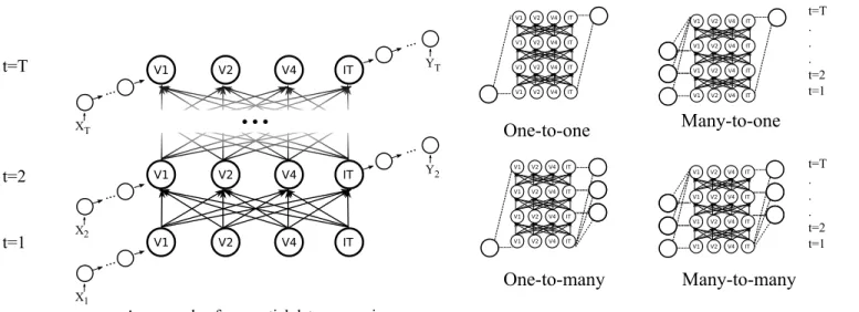
V1 V2 V4 IT t=T t=2 t=1 V1 V2 V4 IT V1 V2 V4 IT...
... X ... X ... X ... T 2 1 YT ... Y2An example of sequential data processing
One-to-one
One-to-many
Many-to-one
Many-to-many
t=T . . . t=2 t=1 t=T . . . t=2 t=1 V1 V2 V4 IT V1 V2 V4 IT V1 V2 V4 IT V1 V2 V4 IT V1 V2 V4 IT V1 V2 V4 IT V1 V2 V4 IT V1 V2 V4 IT V1 V2 V4 IT V1 V2 V4 IT V1 V2 V4 IT V1 V2 V4 IT V1 V2 V4 IT V1 V2 V4 IT V1 V2 V4 IT V1 V2 V4 ITFigure 5: Our model supports sequential inputs/outputs, which includes one-to-one, many-to-one, one-to-many and many-to-many input-output mappings.
4
Related Work
Deep Recurrent Neural Networks: Our final model is deep and similar to a stacked RNN [27, 5, 7] with several main differences: 1. our model has feedback transitions between hidden layers and self-transition from each hidden layer to itself. 2. our model has identity shortcut mappings inspired by residual learning. 3. our transition functions are deep and convolutional.
As suggested by [23], the term depth in RNN could also refer to input-to-hidden, hidden-to-hidden or hidden-to-output connections. Our model is deep in all of these senses. See Section 3.2.
Recursive Neural Networks and Convolutional Recurrent Neural Networks: When unfolding RNN
into a feedforward network, the weights of many layers are tied. This is reminiscent of Recursive Neural Networks (Recursive NN), first proposed by [29]. Recursive NN are characterized by applying same operations recursively on a structure. The convolutional version was first studied by [4]. Subsequent related work includes [24] and [19]. One characteristic distinguishes our model and residual learning from Recursive NN and convolutional recurrent NN is whether there are identity shortcut mappings. This discrepancy seems to account for the superior performance of residual learning and of our model over the latters.
A recent report [3] we became aware of after we finished this work discusses the idea of imitating cortical feedback by introducing loops into neural networks.
A Highway Network [30] is a feedforward network inspired by Long Short Term Memory [11] featuring more general shortcut mappings (instead of hardwired identity mappings used by ResNet).
5
Experiments
5.1
Dataset and training details
We test all models on the standard CIFAR-10 [15] dataset. All images are 32x32 pixels with color. Data augmentation is performed in the same way as [8].
Momentum was used with hyperparameter 0.9. Experiments were run for 60 epochs with batchsize 64 unless stated otherwise. The learning rates are 0.01 for the first 40 epochs, 0.001 for epoch 41 to 50 and 0.0001 for the last 10 epochs. All experiments used the cross-entropy loss function and softmax for classification. Batch Normalization (BN) [13] is used for all experiments. But the learnable scaling and shifting parameters are not used (except for the last BN layer in the post-net). Network weights were initialized with the method described in [9]. Although we do not expect the initialization to matter as long as batch normalization is used. The implementations are based on MatConvNet[32].
5.2
Experiment A: ResNet with shared weights
5.2.1 Sharing Weights Across Time
We conjecture that the effectiveness of ResNet mainly comes from the fact that it efficiently models the recurrent computations required by the recognition task. If this is the case, one should be able to reinterpret ResNet as a RNN with weight sharing and achieve comparable performance to the original version. We demonstrate various incarnations of this idea and show it is indeed the case.
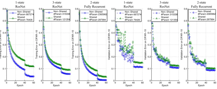
We tested the 1-state and 3-state ResNets described in Figure 3 and 4. The results are shown in Figure 6.
0 20 40 60 0 0.1 0.2 0.3 0.4 0.5 0.6 Epoch Training Error on CIFAR−10 Non−Shared #Param 667274 Shared #Param 76426 0 20 40 60 0 0.1 0.2 0.3 0.4 0.5 0.6 Epoch Validation Error on CIFAR−10 Non−Shared #Param 667274 Shared #Param 76426 0 20 40 60 0 0.1 0.2 0.3 0.4 0.5 0.6 Epoch Training Error on CIFAR−10 Non−Shared #Param 315338 Shared #Param 121354 0 20 40 60 0 0.1 0.2 0.3 0.4 0.5 0.6 Epoch Validation Error on CIFAR−10 Non−Shared #Param 315338 Shared #Param 121354 0 20 40 60 0 0.1 0.2 0.3 0.4 0.5 0.6 Epoch Training Error on CIFAR−10 Non−Shared #Param 2365962 Shared #Param 297994 0 20 40 60 0 0.1 0.2 0.3 0.4 0.5 0.6 Epoch Validation Error on CIFAR−10 Non−Shared #Param 2365962 Shared #Param 297994 1-state ResNet 3-state ResNet 2-state Fully Recurrent 1-state ResNet 3-state ResNet 2-state Fully Recurrent
Figure 6: All models are robust to sharing weights across time. This supports our conjecture that deep networks can be well approximated by shallow/moderately-deep RNNs. The transition matrices of all models are shown in Figure 4. “#Param” denotes the number of parameters. The 1-state ResNet has a single state of size 32x32x64 (height × width × #features). It was trained and tested with readout time t=10. The 3-state ResNet has 3 states of size 32x32x16, 16x16x32 and 8x8x64 – there is a transition (via a simple convolution) at time 4 and 8 — each state has a self-transition unrolled 3 times. The 2-state fully recurrent NN has 2 states of the same size: 32x32x64. It was trained and tested with readout time t=10 (same as 1-state ResNet). It is a generalization of and directly comparable with 1-state ResNet, showing the benefit of having more states. The 2-state fully recurrent NN with shared weights and fewer parameters outperforms 1-state and 3-state ResNet with non-shared weights.
5.2.2 Sharing Weights Across All Convolutional Layers (Less Biologically-plausible)
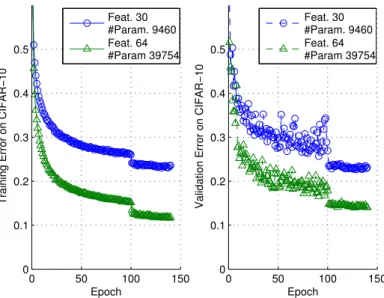
Out of pure engineering interests, one could further push the limit of weight sharing by not only sharing across time but also across states. Here we show two 3-state ResNets that use a single set of convolutional weights across all convolutional layers and achieve reasonable performance with very few parameters (Figure 7).
0 50 100 150 0 0.1 0.2 0.3 0.4 0.5 Epoch
Training Error on CIFAR−10
Feat. 30 #Param. 9460 Feat. 64 #Param 39754
CIFAR−10 with Very Few Parameters
0 50 100 150 0 0.1 0.2 0.3 0.4 0.5 Epoch
Validation Error on CIFAR−10
Feat. 30 #Param. 9460 Feat. 64 #Param 39754
Figure 7: A single set of convolutional weights is shared across all convolutional layers in a 3-state ResNet. The transition (at time t= 4 and 8) between nearby states is a 2x2 max pooling with stride 2. This means that each state has a self-transition unrolled 3 times. “Feat.” denotes the number of feature maps, which is the same across all 3 states. The learning rates were the same as other experiments except that more epochs are used (i.e., 100, 20 and 20).
5.3
Experiment B: Multi-state Fully/Densely Recurrent Neural Networks
5.3.1 Shared vs. Non-shared Weights
Although an RNN is usually implemented with shared weights across time, it is however possible to unshare the weights and use an independent set of weights at every time t. For practical applications, whenever one can have a initial t = 0 and enumerate all possible ts, an RNN with non-shared weights should be feasible, similar to the time-specific batch normalization described in 3.7. The results of 2-state fully recurrent neural networks with shared and non-shared weights are shown in Figure 6.
5.3.2 The Effect of Readout Time
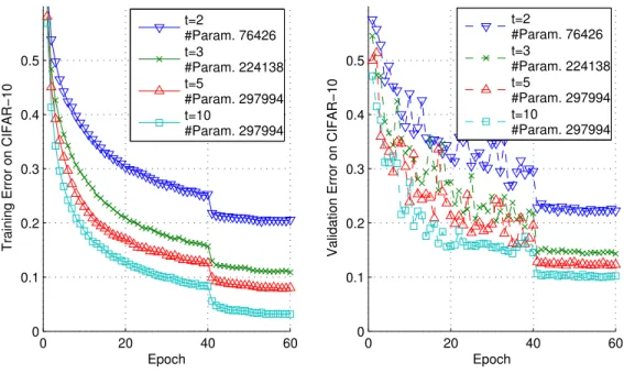
In visual cortex, useful information increases as time proceeds from the onset of the visual stimuli. This suggests that recurrent system might have better representational power as more time is allowed. We tried training and testing the 2-state fully recurrent network with various readout time (i.e., unrolling depth, see Section 3.5) and observe similar effects. See Figure 8.
5.3.3 Larger Models With More States
We have shown the effectiveness of 2-state fully recurrent network above by comparing it with 1-State ResNet. Now we discuss several observations regarding 3-state and 4-state networks.
First, 3-state models seem to generally outperform 2-state ones. This is expected since more parameters are introduced. With a 3-state models with minimum engineering, we were able to get 7.47% validation error on CIFAR-10.
0 20 40 60 0 0.1 0.2 0.3 0.4 0.5 Epoch
Training Error on CIFAR−10
t=2 #Param. 76426 t=3 #Param. 224138 t=5 #Param. 297994 t=10 #Param. 297994
2−State Fully Recurrent NN With Different Readout Time t
0 20 40 60 0 0.1 0.2 0.3 0.4 0.5 Epoch
Validation Error on CIFAR−10
t=2 #Param. 76426 t=3 #Param. 224138 t=5 #Param. 297994 t=10 #Param. 297994
Figure 8: A 2-state fully recurrent network with readout time t=2, 3, 5 or 10 (See Section 3.5 for the definition of readout time). There is consistent performance improvement as t increases. The number of parameters changes since at some t, some recurrent connections have not been contributing to the output and thus their number of parameters are subtracted from the total.
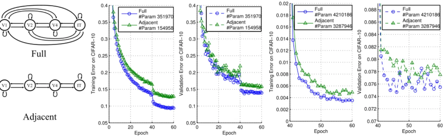
Next, for computational efficiency, we tried only allowing each state to have transitions to adjacent states and to itself by disabling bypass connections (e.g., V1-V3, V2-IT, etc.). In this case, the number of transitions scales linearly as the number of states increases, instead of quadratically. This setting performs well with 3-state networks and slightly less well with 4-state networks (perhaps as a result of small feature/parameter sizes). With only adjacent connections, the models are no longer fully recurrent.
Finally, for 4-state fully recurrent networks, the models tend to become overly computationally heavy if we train it with large t or large number of feature maps. With small t and feature maps, we have not achieved better performance than 3-state networks. Reducing the computational cost of training multi-state densely recurrent networks would be an important future work.
For experiments in this subsection, we choose a moderately deep pre-net of three 3x3 convolutional layers to model the layers between retina and V1: Conv-BN-ReLU-Conv-BN-ReLU-Conv. This is not essential but outperforms shallow pre-net slightly (within 1% validation error).
The results are shown in Figure 9.
5.3.4 Generalization Across Readout Time
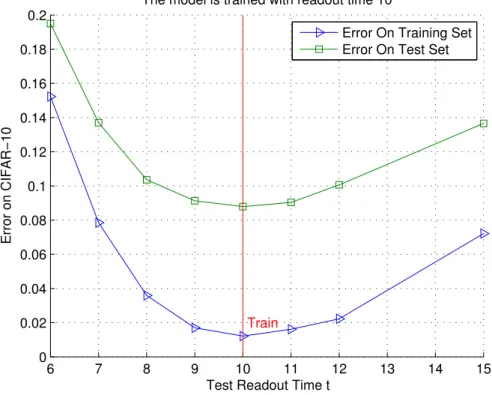
As an RNN, our model supports training and testing with different readout time. Based on our theoretical analyses in Section 2.2, the representation is usually not guaranteed to converge when running a model with time t → ∞. Nevertheless, the model exhibits good generalization over time. Results are shown in Figure 10. As a minor detail, the model in this experiment has only adjacent connections and does not have any self-transition, but we do not expect this to affect the conclusion.
V1 V2 V4 IT V1 V2 V4 IT Full Adjacent 40 50 60 0 0.002 0.004 0.006 0.008 0.01 0.012 0.014 0.016 0.018 0.02 Epoch Training Error on CIFAR−10 Full #Param 4210186 Adjacent #Param 3287946
3−State Fully/Densely Recurrent Neural Networks
40 50 60 0.07 0.072 0.074 0.076 0.078 0.08 0.082 0.084 0.086 0.088 Epoch Validation Error on CIFAR−10 Full #Param 4210186 Adjacent #Param 3287946 0 20 40 60 0.05 0.1 0.15 0.2 0.25 0.3 0.35 0.4 Epoch Training Error on CIFAR−10 Full #Param 351970 Adjacent #Param 154958
4−State Fully/Densely Recurrent Neural Networks (Small Model)
0 20 40 60 0.05 0.1 0.15 0.2 0.25 0.3 0.35 0.4 Epoch Validation Error on CIFAR−10 Full #Param 351970 Adjacent #Param 154958
Figure 9: The performance of 4-state and 3-state models. The state sizes of the 4-state model are: 32x32x8, 16x16x16, 8x8x32, 4x4x64. The state sizes of the 3-state model are: 32x32x64, 16x16x128, 8x8x256. 4-state models are small since they are computationally heavy. The readout time is t=5 for both models. All models are time-invariant systems (i.e., weights are shared across time).
6
Discussion
The dark secret of Deep Networks: trying to imitate Recurrent Shallow Networks?
A radical conjecture would be: the effectiveness of most of the deep feedforward neural networks, including but not limited to ResNet, can be attributed to their ability to approximate recurrent computations that are prevalent in most tasks with larger t than shallow feedforward networks. This may offer a new perspective on the theoretical pursuit of the long-standing question “why is deep better than shallow” [22, 21].
Equivalence between Recurrent Networks and Turing Machines
Dynamical systems (in particular discrete time systems, that is difference equations) are Turing universal (the game “Life" is a cellular automata that has been demonstrated to be Turing universal). Thus dynamical systems such as the feedback systems we discussed can be equivalent to Turing machine. This offers the possibility of representing a computation more complex than a single (for instance boolean) function with the same number of learnable parameters. Consider for instance the powercase of learning a mapping F between an input vector x and an output vector y = F (x) that belong to the same n-dimensional space. The output can be thought as the asymptotic states of the discrete dynamical system obtained iterating some map f . We expect that in many cases the dynamical system that asymptotically performs the mapping may have a much simpler structure than the direct mapping F . In other words, we expect that the mapping f such that f(n)(x) = F (x) for appropriate, possibly very large n can be much simpler than the mapping F (here f(n)means the n-th iterate of the map f ).
Empirical Finding: Recurrent Network or Residual Networks with weight sharing work well
Our key finding is that multi-state time-invariant recurrent networks seem to perform as well as very deep residual networks (each state corresponds to a cortical area) without shared weights. On one hand this is surprising because the number of parameters is much reduced. On the other hand a recurrent network with fixed parameters can be equivalent to a Turing machine and maximally powerful.
Conjecture about Cortex and Recurrent Computations in Cortical Areas
Most of the models of cortex that led to the Deep Convolutional architectures and followed them – such as the Neocognitron [6], HMAX [26] and more recent models [1] – have neglected the layering in each cortical area and the feedforward and recurrent connections within each area and between them. They also neglected the time evolution of selectivity and invariance in each of the areas. The conjecture we propose in this paper changes this picture quite drastically and makes several interesting predictions. Each area corresponds to a recurrent network and thus to a
6 7 8 9 10 11 12 13 14 15 0 0.02 0.04 0.06 0.08 0.1 0.12 0.14 0.16 0.18 0.2
Test Readout Time t
Error on CIFAR−10
The model is trained with readout time 10
Train
Error On Training Set Error On Test Set
Figure 10: Training and testing with different readout time. A 3-state recurrent network with adjacent connections is trained with readout time t=10 and test with t=6,7,8,9,10,11,12 and 15.
system with a temporal dynamics even for flashed inputs; with increasing time one expects asymptotically better performance; masking with a mask an input image flashed briefly should disrupt recurrent computations in each area; performance should increase with time even without a mask for briefly flashed images. Finally, we remark that our proposal, unlike relatively shallow feedforward models, implies that cortex, and in fact its component areas are computationally as powerful a universal Turing machines.
Acknowledgments
This work was supported by the Center for Brains, Minds and Machines (CBMM), funded by NSF STC award CCF – 1231216.
References
References
[1] Using goal-driven deep learning models to understand sensory cortex. Nature Neuroscience, 19,3:356–365, 2016. [2] Christian Büchel and KJ Friston. Modulation of connectivity in visual pathways by attention: cortical
interactions evaluated with structural equation modelling and fmri. Cerebral cortex, 7(8):768–778, 1997. [3] Isaac Caswell, Chuanqi Shen, and Lisa Wang. Loopy neural nets: Imitating feedback loops in the human brain.
CS231n Report, Stanford, http://cs231n.stanford.edu/reports2016/110_Report.pdf. Google Scholar time stamp: March 25th, 2016.
[4] David Eigen, Jason Rolfe, Rob Fergus, and Yann LeCun. Understanding deep architectures using a recursive convolutional network. arXiv preprint arXiv:1312.1847, 2013.
[5] Salah El Hihi and Yoshua Bengio. Hierarchical recurrent neural networks for long-term dependencies. Citeseer. [6] Kunihiko Fukushima. Neocognitron: A self-organizing neural network model for a mechanism of pattern
recognition unaffected by shift in position. Biological Cybernetics, 36(4):193–202, April 1980.
[7] Alex Graves. Generating sequences with recurrent neural networks. arXiv preprint arXiv:1308.0850, 2013. [8] Kaiming He, Xiangyu Zhang, Shaoqing Ren, and Jian Sun. Deep residual learning for image recognition. arXiv
preprint arXiv:1512.03385, 2015.
[9] Kaiming He, Xiangyu Zhang, Shaoqing Ren, and Jian Sun. Delving deep into rectifiers: Surpassing human-level performance on imagenet classification. In Proceedings of the IEEE International Conference on Computer Vision, pages 1026–1034, 2015.
[10] Kaiming He, Xiangyu Zhang, Shaoqing Ren, and Jian Sun. Identity mappings in deep residual networks. arXiv preprint arXiv:1603.05027, 2016.
[11] Sepp Hochreiter and Jürgen Schmidhuber. Long short-term memory. Neural computation, 9(8):1735–1780, 1997.
[12] JM Hupe, AC James, BR Payne, SG Lomber, P Girard, and J Bullier. Cortical feedback improves discrimination between figure and background by v1, v2 and v3 neurons. Nature, 394(6695):784–787, 1998.
[13] Sergey Ioffe and Christian Szegedy. Batch normalization: Accelerating deep network training by reducing internal covariate shift. arXiv preprint arXiv:1502.03167, 2015.
[14] Minami Ito and Charles D Gilbert. Attention modulates contextual influences in the primary visual cortex of alert monkeys. Neuron, 22(3):593–604, 1999.
[15] Alex Krizhevsky. Learning multiple layers of features from tiny images, 2009.
[16] Alex Krizhevsky, Ilya Sutskever, and Geoffrey E Hinton. Imagenet classification with deep convolutional neural networks. In Advances in neural information processing systems, pages 1097–1105, 2012.
[17] Victor AF Lamme, Hans Super, and Henk Spekreijse. Feedforward, horizontal, and feedback processing in the visual cortex. Current opinion in neurobiology, 8(4):529–535, 1998.
[18] César Laurent, Gabriel Pereyra, Philémon Brakel, Ying Zhang, and Yoshua Bengio. Batch normalized recurrent neural networks. arXiv preprint arXiv:1510.01378, 2015.
[19] Ming Liang and Xiaolin Hu. Recurrent convolutional neural network for object recognition. In Proceedings of the IEEE Conference on Computer Vision and Pattern Recognition, pages 3367–3375, 2015.
[20] Qianli Liao, Joel Z Leibo, and Tomaso Poggio. How important is weight symmetry in backpropagation? arXiv preprint arXiv:1510.05067, 2015.
[21] Hrushikesh Mhaskar, Qianli Liao, and Tomaso Poggio. Learning real and boolean functions: When is deep better than shallow. arXiv preprint arXiv:1603.00988, 2016.
[22] Guido F Montufar, Razvan Pascanu, Kyunghyun Cho, and Yoshua Bengio. On the number of linear regions of deep neural networks. In Advances in neural information processing systems, pages 2924–2932, 2014.
[23] Razvan Pascanu, Caglar Gulcehre, Kyunghyun Cho, and Yoshua Bengio. How to construct deep recurrent neural networks. arXiv preprint arXiv:1312.6026, 2013.
[24] Pedro HO Pinheiro and Ronan Collobert. Recurrent convolutional neural networks for scene parsing. arXiv preprint arXiv:1306.2795, 2013.
[25] Rajesh PN Rao and Dana H Ballard. Predictive coding in the visual cortex: a functional interpretation of some extra-classical receptive-field effects. Nature neuroscience, 2(1):79–87, 1999.
[26] M Riesenhuber and T Poggio. Hierarchical models of object recognition in cortex. Nature Neuroscience, 2(11):1019–1025, November 1999.
[27] Jürgen Schmidhuber. Learning complex, extended sequences using the principle of history compression. Neural Computation, 4(2):234–242, 1992.
[28] Thomas Serre, Aude Oliva, and Tomaso Poggio. A feedforward architecture accounts for rapid categorization. Proceedings of the National Academy of Sciences of the United States of America, 104(15):6424–6429, 2007. [29] Richard Socher, Cliff C Lin, Chris Manning, and Andrew Y Ng. Parsing natural scenes and natural language
with recursive neural networks. In Proceedings of the 28th international conference on machine learning (ICML-11), pages 129–136, 2011.
[30] Rupesh Kumar Srivastava, Klaus Greff, and Jürgen Schmidhuber. Highway networks. arXiv preprint arXiv:1505.00387, 2015.
[31] Simon Thorpe, Denis Fize, Catherine Marlot, et al. Speed of processing in the human visual system. nature, 381(6582):520–522, 1996.
[32] Andrea Vedaldi and Karel Lenc. Matconvnet: Convolutional neural networks for matlab. In Proceedings of the 23rd Annual ACM Conference on Multimedia Conference, pages 689–692. ACM, 2015.
[33] D.L.K. Yamins and J.D. Dicarlo. Using goal-driven deep learning models to understand sensory cortex, 2016. [34] Matthew D Zeiler, Dilip Krishnan, Graham W Taylor, and Rob Fergus. Deconvolutional networks. In Computer
Vision and Pattern Recognition (CVPR), 2010 IEEE Conference on, pages 2528–2535. IEEE, 2010.
A
An Illustrative Comparison of a Plain RNN and a ResNet
Unfold
K
Plain RNNh
XK
h
h
K
X X 0 0 1 1K
h
...
K
h
0h
1...
X0h2
ResNet With Weight Sharing + +K
h2
ResNet Recurrent Form Unrolled RNN +Figure 11: A ResNet can be reformulated into a recurrent form that is almost identical to a conventional RNN.
B
Inhomogeneous, Time-invariant ResNet
The inhomogeneous, time-invariant version of ResNet is shown in Figure 12. Let K0= K + I, asymptotically we have:
h = Ix + K0h (7)
(I − K0)h = x (8)
h = (I − K0)−1x (9)
The power series expansion of above equation is:
h = (I − K0)−1x = (I + K0+ K0◦ K0+ K0◦ K0◦ K0+ ...)x (10)
Inhomogeneous, time-invariant version of ResNet corresponds to the standard ResNet with shared weights and shortcut connections from input to every layer. If the model has only one state, it is experimentally observed that these shortcuts undesirably add raw inputs to the final representations and degrade the performance. However, if
I I I
I
+
h
x
x
0h
+ + +...
(A) ResNet with shared weights
and shortcuts from input to all layers
K'
8
h
0h
1h
2xt=x0
K' K' K'K'=K+I
(B) Folded
Fold
Unfold
Figure 12: Inhomogeneous, Time-invariant ResNet
the model has multiple states (like the visual cortex), it might be biologically-plausible for the first state (V1) to receive constant inputs from the pre-net (retina and LGN). Figure 13 shows the performance of an inhomogeneous 3-state recurrent network in comparison with homogeneous ones.
Input t=4 t=3 t=2 t=1 Input Homogeneous Inhomogeneous 40 45 50 55 60 0 0.002 0.004 0.006 0.008 0.01 0.012 0.014 0.016 0.018 0.02 Epoch Training Error on CIFAR−10 Full #Param 4210186 Adjacent #Param 3287946 Adjacent, inhomogeneous #Param 3287946
3−State Fully/Densely Recurrent Neural Networks
40 45 50 55 60 0.07 0.072 0.074 0.076 0.078 0.08 0.082 0.084 0.086 0.088 Epoch Validation Error on CIFAR−10 Full #Param 4210186 Adjacent #Param 3287946 Adjacent, inhomogeneous #Param 3287946 V1 V2 V4 IT V1 V2 V4 IT V1 V2 V4 IT V1 V2 V4 IT V1 V2 V4 IT V1 V2 V4 IT V1 V2 V4 IT V1 V2 V4 IT