Speech synthesis using recurrent neural networks

(1)

Universit´e de Montr´eal

Speech Synthesis Using Recurrent Neural Networks

par Jos´e Manuel Rodr´ıguez Sotelo

Département d’informatique et de recherche opérationnelle Faculté des arts et des sciences

Mémoire présenté à la Faculté des arts et des sciences en vue de l’obtention du grade de Maˆıtre ès sciences (M.Sc.)

en informatique

D´ecembre, 2016

c

(2)

Résumé

Les réseaux neuronaux récurrents sont des outils efficaces pour modeler les données à structure séquentielle. Dans ce mémoire, nous décrivons comment les utiliser pour la synthèse vocale.

Nous commen¸cons avec une introduction `a l’apprentissage automatique et aux r´eseaux neuronaux dans le chapitre1.

Dans le chapitre 2, nous développons un gradient algorithmique stochastique automatique ayant pour effet de réduire le poids des recherches extensives hyper-paramétrées pour l’optimisateur. L’algorithme proposé exploite un estimateur de courbure du coût de la fonction de moindre variance, et utilise celui-ci pour obtenir un taux d’apprentissage adaptatif qui soit automatiquement calibré pour chaque paramètre.

Dans le chapitre 3, nous proposons un modèle innovateur pour la génération audio inconditionnelle, basée sur la génération d’un seul échantillon audio à la fois. Nous montrons que notre modèle, qui prend avantage de la combination de mo-dules sans mémoire (notamment les perceptrons autorégressifs à plusieurs couches et les réseaux de neurones récurrents dans une structure hiérarchique), est capable de capturer les sources de variation sous-jacentes dans les séquences temporelles, et ce, sur de très longs laps de temps, sur trois ensembles de données de nature différente. Les résultats de l’évaluation humaine à l’écoute des échantillons générés semblent indiquer que notre modèle est préféré à d’autres modèles de compéti-teurs. Nous montrons aussi comment chaque composante du modèle contribue à ces performances.

Dans le chapitre 4, nous présentons un modèle d’encodeur-décodeur focalisé sur la synthèse vocale. Notre modèle apprend à produire les caractéristiques acoustiques à partir d’une séquence de phonèmes ou de lettres. L’encodeur se constitue d’un réseau neuronal récurrent bidirectionnel acceptant des entrées sous forme de texte ou de phonèmes. Le décodeur se constitue, pour sa part, d’un réseau neuronal récurrent avec attention produisant les caractéristiques acoustiques. Par ailleurs, nous adaptons ce modèle, afin qu’il puisse réaliser la synthèse vocale de plusieurs individus, et nous la testons en anglais et en espagnol.

Finalement, nous effectuons une réflection sur les résultats obtenus dans ce mé-moire, afin de proposer de nouvelles pistes de recherche.

(3)

(4)

Summary

Recurrent neural networks are useful tools to model data with sequential struc-ture. In this work, we describe how to use them for speech synthesis.

We start with an introduction to machine learning and neural networks in Chap-ter 1.

In Chapter 2, we develop an automatic stochastic gradient algorithm which reduces the burden of extensive hyper-parameter search for the optimizer. Our proposed algorithm exploits a lower variance estimator of curvature of the cost function and uses it to obtain an automatically tuned adaptive learning rate for each parameter.

In Chapter 3, we propose a novel model for unconditional audio generation based on generating one audio sample at a time. We show that our model, which profits from combining memory-less modules, namely autoregressive multilayer per-ceptrons, and stateful recurrent neural networks in a hierarchical structure is able to capture underlying sources of variation in the temporal sequences over very long time spans, on three datasets of different nature. Human evaluation on the gener-ated samples indicate that our model is preferred over competing models. We also show how each component of the model contributes to the exhibited performance. In Chapter 4, we present Char2Wav, an end-to-end model for speech synthesis. Char2Wav has two components: a reader and a neural vocoder. The reader is an encoder-decoder model with attention. The encoder is a bidirectional recurrent neural network (RNN) that accepts text or phonemes as inputs, while the decoder is a recurrent neural network with attention that produces vocoder acoustic features. Neural vocoder refers to a conditional extension of SampleRNN which generates raw waveform samples from intermediate representations. We show results in English and Spanish. Unlike traditional models for speech synthesis, Char2Wav learns to produce audio directly from text.

Finally, we reflect on the results obtained in this work and propose future di-rections of research in the area.

Keywords: neural networks, machine learning, deep learning, representation learning, speech synthesis, signal processing, optimization

(5)

List of Figures

1.1 Generative models. Figure from ?. . . 3

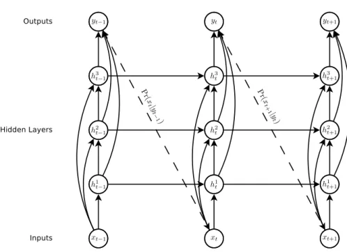
1.2 Deep recurrent neural network. The dashed lines represent sampling from a distribution. Figure from ?. . . 6

2.1 Baseline comparison against Adam. AdaSecant performs as well as Adam with a carefully tuned learning rate. . . 24

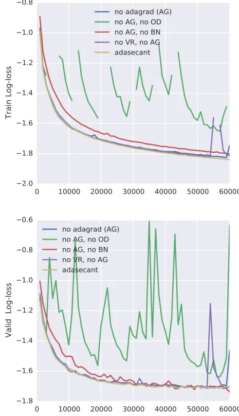
2.2 Deactivating one component at a time. BN provides a small but constant advantage in performance. OD is important for the algo-rithm. Deactivating it makes training more noisy and unstable and gives worse results. Deactivating VR also makes training unstable. . 25

2.3 Learning curves for the very well-tuned Adam vs AdaSecant algo-rithm without any hyperparameter tuning. AdaSecant performs very close to the very well-tuned Adam on PTB character-level language modeling task. This shows us the robustness of the algorithm to its hyperparameters. . . 26

2.4 Comparison of different stochastic gradient algorithms on MNIST with Maxout Networks. Both a) and b) are trained with dropout and maximum column norm constraint regularization on the weights. Networks are initialized with weights sampled from a Gaussian dis-tribution with 0 mean and standard deviation of 0.05. In both exper-iments, the proposed algorithm, Adasecant, seems to be converging faster and arrives to a better minima in training set. We trained both networks for 350 epochs over the training set. . . 26

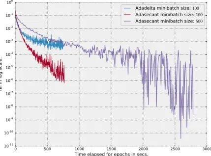
2.5 In this plot, we compared AdaSecant trained by using minibatch size of 100 and 500 with adadelta using minibatches of size 100. We performed these experiments on MNIST with 2-layer maxout MLP using dropout.. . . 27

2.6 No variance reduction comparison. . . 28

2.7 No Adagrad comparison. . . 29

2.8 No block normalization comparison. . . 30

2.9 No outlier detection comparison.. . . 31

3.1 Snapshot of the unrolled model at timestep i with K = 3 tiers. As a simplification only one RNN and up-sampling ratio r = 4 is used for all tiers. . . 36

(8)

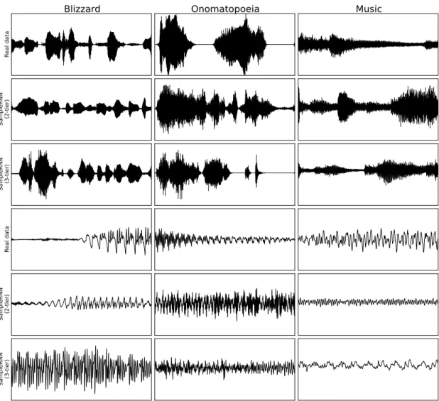
3.2 Examples from the datasets compared to samples from our models. In the first 3 rows, 2 seconds of audio are shown. In the bottom 3 rows, 100 milliseconds of audio are shown. Rows 1 and 4 are ground truth from which one can see how the datasets look different and have complex structure in low resolution which the frame-level component of the SampleRNN is designed to capture. Samples also to some extent mimic the same global structure. At the same time, zoomed-in samples of our model shows that it can perfectly resemble the high resolution structure present in the data as well. . . 42

3.3 Pairwise comparison of 4 best models based on the votes from listen-ers conducted on samples generated from models trained on Blizzard dataset. . . 45

3.4 Pairwise comparison of 3 best models based on the votes from listen-ers conducted on samples generated from models trained on Music dataset. . . 46

4.1 Char2Wav: An end-to-end speech synthesis model. . . 54

4.2 Sample from the model conditioned on English phonemes. The model was trained on the VCTK dataset. . . 58

4.3 Sample from the model conditioned on English text. The model was trained on the VCTK dataset. . . 59

4.4 Sample from the model conditioned on Spanish text. The model was trained on the DIMEX-100 dataset (?). . . 60

4.5 Results of the preference test. Area on the graph corresponds to the proportion of participants that preferred the listed model.. . . 61

4.6 Results of the intelligibility test. Word error rates are reported for the outputs of Char2Wav, original speech processed by the WORLD vocoder, and reader with vocoder output. . . 61

(9)

List of Tables

2.1 Summary of results for the handwriting experiment. We report the best validation log-loss that we found for each model using early stopping. We also report the corresponding train log-loss. In all cases, the log-loss is computed per data point. . . 20

3.1 Test NLL in bits for three presented datasets. . . 41

3.2 Average NLL on Blizzard test set for real-valued models. . . 41

3.3 Effect of subsequence length on NLL (bits per audio sample) com-puted on the Blizzard validation set. . . 42

3.4 Test (validation) set NLL (bits per audio sample) for Blizzard. Vari-ants of SampleRNN are provided to compare the contribution of each component in performance.. . . 43

(10)

List of Abbreviations

AE Auto-Encoder

GD Gradient Descent GRU Gated Recurrent Unit GMM Gaussian Mixture Model HMM Hidden Markov Model KLD Kullback-Liebler Divergence LSTM Long-Short Term Memory

MLE Maximum Likelihood Estimation MLP Multi-Layer Perceptron

MSE Mean Squared Error NLL Negative Log-Likelihood RNN Recurrent Neural Network SGD Stochastic Gradient Descent SP Signal Processing

SS Speech Synthesis

(11)

1

_Introduction

To conclude what does learning really mean would definitely make your favorite philosopher happy. Our concept of learning contains different processes that make the definition unclear. Some of the possible definitions of learning are: acquire knowledge of something by experience or by study, add something the memory, or modify the behavior based on experience.

The ability to learn is the single most important quality that makes us thrive in our environment. It is the ability that allows us to adapt our behavior to respond to threats and to get skills that allow our survival. Learning is such an important part of our lives that without it we could not communicate, we could not make complex tools, we could not transfer our knowledge to new generations, etc. In a few words, if we were not able to learn new things, we would be extinct.

Learning is so rooted in our brains that we do not even need to think about it for it to happen. Usually, when you learn a new skill, you do not think about how to learn it. In part because of this, we do not have a clear understanding of how learning works inside our brains. Hence, it is challenging to provide this amazing skill to the devices that we create. By giving machines the ability to learn, we hope that, eventually, they will be able to solve the problems that we have not found the solution of.

This is a thesis about machine learning. In particular, we tackle the problem of applying modern machine learning techniques to speech synthesis (SS). Speech synthesis, also known as Text-to-Speech (TTS), consists on finding the mapping from text to audio signal. In the traditional approach, developing a new SS system requires specialized linguistic knowledge and handcrafted features. In this work, we develop a new algorithm that uses deep learning to make this process much simpler. In summary, this thesis proposes a new solution to an old problem: speech synthesis.

(12)

1.1 Machine Learning

Machine learning tries to provide the ability to learn to computers. In machine learning, we usually do not know how to describe the solution to a problem. Instead, we give our models the ability to learn the solution to the problem by themselves. The motivation for this is simple: If we are able to teach the computers how to solve problems by themselves, they will be able to solve unsolved problems.

The idea that computers can learn to solve problems by themselves is old. As ? describe, during the first years of the field of Artificial Intelligence (1952 -1969), it was believed that in a few years computers would become better than humans to perform complex tasks. However, this optimism was over because of the limit in computational resources of the time. Even more, confidence in the field plummeted. People started doubting that computers would be able to learn how to solve difficult problems. Regardless of the limitations in the computational power of the time, these years were fruitful in ideas about learning. Ideas from other fields, like psychology, were adopted. Therefore, some of the techniques developed in the field come from models to understand human or animal behavior.

Recently, there has been an explosion in the computational power and the data available. These two factors have transformed the field.

1.2 Generative Models

Every adult human has an incredible amount of information about the world that we live in. We understand that the world has 3 dimensions. We understand that we interact with objects that continuously move. We know how to navigate our world, how to communicate with other humans. We learn from historic recordings what happened in our past. We have created tools, like the Internet, that allows us to learn about the present.

Most of this huge amount of information is easily accessible in the Internet or in the physical World. However, it is no trivial to develop models and algorithms that can analyze and understand this treasure trove of data. Generative models are one of the most promising approaches towards this goal (?).

(13)

(14)

find the parameters θ of a neural network that minimize a cost function J(θ). The function J(θ) usually includes a measure of performance in the desired task as well as additional regularization terms.

J(θ) = E(x,y)∼ˆpdataL(f (x; θ), y) (1.1)

where L is a per-example cost function, f (x; θ) is the predicted output when the input is x, and ˆpdata the empirical distribution.

In contrast with the field of optimization, in machine learning the goal in and of itself is not to minimize the cost function. Instead, the goal is to have a good performance on unobserved examples. That is, our goal is to optimize:

J∗(θ) = E(x,y)∼pdataL(f (x; θ), y) (1.2)

where pdata is the data generating distribution. Since we do not know pdata in

most real world applications, we work with a training set of examples. This makes machine learning different.

Overfitting is a measure of the difference between the goals of optimization and machine learning. Since we work with only a training set of examples, if we use high capacity models and powerful optimization algorithms we can simply memo-rize the training set. Because of this, machine learning makes us of regularization techniques like early stopping. Furthermore, the most effective modern optimiza-tion algorithms are based on gradient descent. Since many useful loss funcoptimiza-tions do not have useful derivatives, we often rely on surrogate loss functions which act as a proxy.

In Chapter 2, we develop an automatic stochastic gradient algorithm which reduces the burden of extensive hyper-parameter search for the optimizer. Our proposed algorithm exploits a lower variance estimator of curvature of the cost function and uses it to obtain an automatically tuned adaptive learning rate for each parameter.

(15)

1.4 Neural Networks

Deep learning is a subset of Machine Learning that focuses on Neural Networks. An artificial neuron is a simple model of how a neuron in the brain works. In the brain, neurons respond to electric impulses sent by neighboring neurons. In the same way, a neural network is a model that connects many single neurons. Furthermore, deep learning got its name from the fact that we usually organize the neurons in layers and we transform the input layer-by-layer. This is equivalent to composing together many different functions. In particular, we model neural networks using the following equations:

h0 = x (1.3)

hi = gi(wTi hi−1+ bi) ∀i ∈ 1, ..., N (1.4)

where x is the input, N is the number of layers, and gi is the activation function of

the i-th layer. This model is called a feed-forward neural network or deep neural network (DNN). Where N is the depth of the network.

1.5 Recurrent Neural Networks

Recurrent neural networks (RNN) have been proved to be a powerful tool to model sequences like text (?), handwriting (?) and more. In the traditional gen-erative model, a RNN is trained to model a sequence by predicting one step at a time and predicting what comes next. The RNN is trained to use past information to estimate the parameters of a distribution of the next step of the sequence. At testing time, the next step is sampled from this distribution and is taken as truth for the following computations as in Figure1.2

P(y) = P(y1) T Y t=2 P(yt|y1, ..., yt−1) (1.5) = P(y1) T Y t=2 P(yt|ht) (1.6) hi_t = g(Whhhi_t−1+ Wihhi−1t ) (1.7)

(16)

Figure 1.2 – Deep recurrent neural network. The dashed lines represent sampling from a distribution. Figure from ?.

And we train the network to minimize the negative loglikelihood L(y).

L(y) = −

T

X

t=1

log P (yt|ht) (1.8)

Furthermore, we can condition the sequence generation with additional infor-mation X. In general, X can be anything. For instance, X in image captioning X is an image. In speech recognition X is an audio sequence. In handwriting synthesis and speech synthesis X is a text sequence. Encoder-decoder models (??) were developed to tackle problems where X is a sequence. Therefore, these kinds of models are well-suited for speech synthesis.

A weakness of encoder-decoder models is that they encode all the information about X in a fixed size vector. ? solve this issue using an attention mecha-nism. Since then, attention mechanisms have been widely adopted in the deep and have recently shown great performance on a variety of tasks including handwriting synthesis (?), machine translation (?), image caption generation (?) and speech recognition (??).

(17)

1.6 Speech synthesis

Audio generation is a challenging task at the core of many problems of interest, such as text-to-speech synthesis, music synthesis and voice conversion. The par-ticular difficulty of audio generation is that there is often a very large discrepancy between the dimensionality of the the raw audio signal and that of the effective semantic-level signal. Consider the task of speech synthesis, where we are typically interested in generating utterances corresponding to full sentences. Even at a rel-atively low sample rate of 16kHz, on average we will have 6,000 samples per word generated.1

Speech Synthesis consists on the mapping from text to audio signal. It has two main goals, intelligibility and naturalness. Traditionally, speech synthesis has been solved by dividing the problem in two stages. The first stage, known as the frontend, transforms the text into linguistic features. These linguistic features usually include phone, syllable, word, phrase and utterance-level features (?) (e.g. phone identities, syllable stress, the number of syllables in a word, and position of the current syllable in a phrase) with additional frame position and phone duration features (??). These features are obtained by forced alignment at the training stage. The second stage, known as the backend, takes as input the linguistic features generated by the frontend and produces the corresponding sound.

There are two popular approaches to tackle the backend problem: concatena-tive synthesis and parametric synthesis. In concatenaconcatena-tive synthesis, the audio is cut into pieces that are labeled with their phoneme or other linguistic information. At generation time, we find appropriate speech units in the database. Finally, we use signal processing techniques to paste the chunks together. In parametric speech synthesis (?), we extract vocoder parameters from speech signals. Then, we train a generative model that will output these parameters given the desired linguistic features. A maximum likelihood parameter estimation algorithm is used to gener-ate the parameters. Finally, the waveform is constructed using the vocoder. The conventional approach to statistical parametric speech synthesis uses tree-clustered context-dependent hidden Markov models (HMMs) to model the probability

den-1. Statistics based on the average speaking rate of a set of TED talk speakers http:// sixminutes.dlugan.com/speaking-rate/

(18)

sities of vocoder parameters. For a more detailed review of traditional models of speech synthesis, we recommend (?).

Recently, there have been advances by using neural networks to model vocoder parameters. ? propose using (feed-forward) Deep Neural Networks to model the acoustic parameters of the vocoder. ? present a lightweight model for mobile devices using Recurrent Neural Networks (RNN). ?? present a comprehensive review of the progress made by using neural networks for acoustic modeling.

Traditionally, the high-dimensionality of raw audio signal is dealt with by first compressing it into spectral or hand-engineered features and defining the genera-tive model over these features. However, when the generated signal is eventually decompressed into audio waveforms, the sample quality is often degraded and re-quires extensive domain-expert corrective measures. This results in complicated signal processing pipelines that are to adapt to new tasks or domains. Further-more, there have been a few recent attempts to take away the vocoder and model the raw waveform directly (???).

In Chapter3, we propose a novel model for unconditional audio generation based on generating one audio sample at a time: SampleRNN. We show that our model, which profits from combining memory-less modules, namely autoregressive multi-layer perceptrons, and stateful recurrent neural networks in a hierarchical structure is able to capture underlying sources of variation in the temporal sequences over very long time spans, on three datasets of different nature. Human evaluation on the generated samples indicate that our model is preferred over competing mod-els. We also show how each component of the model contributes to the exhibited performance.

Furthermore, in Chapter 4, we present Char2Wav, an end-to-end model for speech synthesis. Char2Wav has two components: a reader and a neural vocoder. The reader is an encoder-decoder model with attention. The encoder is a bidi-rectional recurrent neural network (RNN) that accepts text or phonemes as in-puts, while the decoder is a recurrent neural network with attention that produces vocoder acoustic features. Neural vocoder refers to a conditional extension of Sam-pleRNN which generates raw waveform samples from intermediate representations.

(19)

2

_Adasecant

A Robust Adaptive Stochastic Gradient Method for Deep Learning. Caglar Gulcehre*, Jose Sotelo*, Marcin Moczulski, Yoshua Bengio.1

Personal Contribution. My main contribution to the project was the ablation study. I joined this project after the algorithm had already been theoretically devel-oped. The algorithm was developed by Caglar and Marcin supervised by Yoshua. They presented a preliminary v ersion of this paper in the NIPS Workshop in Optimization, 2015. I joined the team to update the paper with the comments received in the workshop. For this, I coded the handwriting synthesis experiment and performed the ablation study and the comparison with Adasecant. Further-more, I rewrote most of the Results section. Finally, I did minor edits of the other sections. This chapter was accepted in the IJCNN, 2017.

Affiliations

Caglar Gulcehre*, MILA, Département d’Informatique et de Recherche Opéra-tionnelle, Université de Montréal

Jose Sotelo*, MILA, Département d’Informatique et de Recherche Opérationnelle, Université de Montréal

Marcin Moczulski, University of Oxford

Yoshua Bengio, MILA, Département d’Informatique et de Recherche Opéra-tionnelle, Université de Montréal, CIFAR Senior Fellow

Funding We thank the computational resources provided by Compute Canada and Calcul Qu´ebec. This work has been partially supported by NSERC, CIFAR, and Canada Research Chairs, Project TIN2013-41751, grant 2014-SGR-221.

(20)

2.1 Abstract

Stochastic gradient algorithms are the main focus of large-scale optimization problems and led to important successes in the recent advancement of the deep learning algorithms. The convergence of SGD depends on the careful choice of learning rate and the amount of the noise in stochastic estimates of the gradients. In this paper, we propose an adaptive learning rate algorithm, which utilizes stochastic curvature information of the loss function for automatically tuning the learning rates. The information about the element-wise curvature of the loss function is estimated from the local statistics of the stochastic first order gradients. We further propose a new variance reduction technique to speed up the convergence. In our experiments with deep neural networks, we obtained better performance compared to the popular stochastic gradient algorithms.2

2.2 Introduction

We develop an automatic stochastic gradient algorithm which reduces the bur-den of extensive hyper-parameter search for the optimizer. Our proposed algorithm exploits a lower variance estimator of curvature of the cost function and uses it to obtain an automatically tuned adaptive learning rate for each parameter.

In deep learning and numerical optimization literature, several papers suggest using a diagonal approximation of the Hessian (second derivative matrix of the cost function with respect to parameters), in order to estimate optimal learning rates for stochastic gradient descent over high dimensional parameter spaces ???. A fundamental advantage of using such approximation is that inverting such ap-proximation can be a trivial and cheap operation. However generally, for neural networks, the inverse of the diagonal Hessian is usually a bad approximation of the diagonal of the inverse of Hessian. For example, obtaining a diagonal approxima-tion of the Hessian are the Gauss-Newton matrix ? or by finite differences ?. Such estimations may however be very sensitive to the noise coming from the Monte-Carlo estimates of the gradients. ? suggested a reliable way to estimate the local

(21)

curvature in the stochastic setting by keeping track of the variance and average of the gradients.

We propose a different approach: instead of using a diagonal estimate of the Hessian, to estimate curvature along the direction of the gradient and we apply a new variance reduction technique to compute it reliably. By using root mean square statistics, the variance of gradients are reduced adaptively with a simple transformation. We keep track of the estimation of curvature using a technique similar to that proposed by ?, which uses the variability of the expected loss. Standard adaptive learning rate algorithms only scale the gradients, but regular Newton-like second order methods, can perform more complicate transformations, e.g. rotating the gradient vector. Newton and quasi-newton methods can also be invariant to affine transformations in the parameter space. The AdaSecant algorithm is basically a stochastic rank-1 quasi-Newton method. But in comparison with other adaptive learning algorithms, instead of just scaling the gradient of each parameter, AdaSecant can also perform an affine transformation on them.

2.3 Directional Secant Approximation

Directional Newton is a method proposed for solving equations with multiple variables?. The advantage of the directional Newton method compared to Newton’s method is that, it does not require a matrix inversion and still maintains a quadratic rate of convergence.

In this paper, we develop a second-order directional Newton method for non-linear optimization. Step-size tk _{of update ∆}k _{for step k can be written as if it was}

a diagonal matrix:

∆k = −tk⊙ ∇θf(θk), (2.1)

= − diag(tk_)∇

θf(θk), (2.2)

= − diag(dk)(diag(Hdk))−1∇θf(θk). (2.3)

where θk is the parameter vector at update k, f is the objective function and dk _is

(22)

by hi = ∇θ∂f(θ

k

) ∂θi the i

th _{row of the Hessian matrix H and by ∇} θif(θ

k

) the ith

element of the gradient vector at update k, a reformulation of Equation 2.1 for each diagonal element of the step-size diag(tk_{) is:}

∆ki = −t k i∇θif(θ k ), (2.4) = −dki ∇θif(θ k ) hk idk . (2.5) so effectively tki = dk i hk idk . (2.6)

We can approximate the per-parameter learning rate tk

i following ?: tk_i = d k i hk idk , (2.7) = lim |∆k i|→0 ∆k i ∇θif(θ k + ∆k_{) − ∇} θif(θ k ),for every i. (2.8) Please note that alternatively one might use the R-op to compute the Hessian-vector product for the denominator in Equation 2.7 (?).

To choose a good direction dk_{in the stochastic setting, we use block-normalized}

gradient vector that the parameters of each layer is considered as a block and for each weight matrix Wi

k and bias vector bik for θ = {Wki,bik}i=1···k at each layer i

and update k, dk= h dk W0kd k b0k· · · d k bl k i

for a neural network with l layers. The update step is defined as ∆k

i = tkidki. The per-parameter learning rate tki

can be estimated with the finite difference approximation,

tk_i ≈ ∆ k i ∇θif(θ k_{+ ∆}k_{) − ∇} θif(θ k₎, (2.9)

since, in the vicinity of the quadratic local minima,

∇θf(θk+ ∆k) − ∇θf(θk) ≈ Hk∆k, (2.10)

We can therefore recover tk _as

(23)

The directional secant method basically scales the gradient of each parameter with the curvature along the direction of the gradient vector and it is numerically stable.

2.4 Relationship to the Diagonal

Approximation to the Hessian

Our secant approximation of the gradients are also very closely tied to diagonal approximation of the Hessian matrix. Considering that ith _{diagonal entry of the}

Hessian matrix can be denoted as, Hii = ∂

2_f(θ)

∂θ2i . By using the finite differences, it

is possible to approximate this with as in Equation 2.12,ıı

Hii = lim |∆|→0

∇θif(θ + ∆) − ∇θif(θ)

∆i

, (2.12)

Assuming that the diagonal of the Hessian is denoted with A matrix, we can see the equivalence:

A ≈ diag(∇θf(θ + ∆) − ∇θf(θ)) diag(∆)−1. (2.13)

The Equation2.13 can be easily computed in a stochastic setting from the consec-utive minibatches.

2.5 Variance Reduction for Robust Stochastic

Gradient Descent

Variance reduction techniques for stochastic gradient estimators have been well-studied in the machine learning literature. Both ? and ? proposed new ways of dealing with this problem. In this paper, we proposed a new variance reduction technique for stochastic gradient descent that relies only on basic statistics related to the gradient. Let gi refer to the ithelement of the gradient vector g with respect

to the parameters θ and E[·] be an expectation taken over minibatches and different trajectories of parameters.

(24)

We propose to apply the following transformation to reduce the variance of the stochastic gradients: ˜ gi = gi+ γiE[gi] 1 + γi , (2.14)

where γi is strictly a positive real number. Let us note that:

E[ ˜gi] = E[gi] and Var( ˜gi) =

1 (1 + γi)2

Var(gi). (2.15)

The variance is reduced by a factor of (1 + γi)2 compared to Var(gi).

In practice we do not have access to E[gi], therefore a biased estimator gi based

on past values of gi will be used instead. We can rewrite the ˜gi as:

˜ gi = 1 1 + γi gi+ (1 − 1 1 + γi )E[gi], (2.16)

After substitution βi = _1+γ1 i, we will have:

˜

gi = βigi+ (1 − βi)E[gi]. (2.17)

By adapting γior βi, it is possible to control the influence of high variance, unbiased

gi and low variance, biased gion ˜gi. Denoting by g′ the stochastic gradient obtained

on the next minibatch, the γi that well balances those two influences is the one that

keeps the ˜gi as close as possible to the true gradient E[g′i] with g′i being the only

sample of E[g′

i] available. We try to find a regularized βi, in order to obtain a

smoother estimate of it and this yields us a more stable estimate of βi. λ is the

regularization coefficient for β.

arg min

βi

E[|| ˜gi− g′i||22] + λ(βi)2. (2.18)

It can be shown that this a convex problem in βiwith a closed-form solution (details

in appendix) and we can obtain the γi from it:

γi =

E[(gi− gi′)(gi − E[gi])]

E[(gi− E[gi])(gi′− E[gi]))] + λ

, (2.19)

As a result, to estimate γ for each dimension, we keep track of a estimation of

E[(gi−g′i)(gi−E[gi])]

(25)

for the variance reduction is to keep γ positive, to achieve a positive estimate of γ we used the root mean square statistics for the expectations.

2.6 Blockwise Gradient Normalization

It is very well-known that the repeated application of the non-linearities can cause the gradients to vanish ??. Thus, in order to tackle this problem, we nor-malize the gradients coming into each block-layer to have norm 1. Assuming the normalized gradient can be denoted with ˜g, it can be computed as, ˜g = g

||E[g]||2.

We estimate, E[g] via moving averages.

Blockwise gradient normalization of the gradient adds noise to the gradients, but in practice we did not observe any negative impact of it. We conjecture that this is due to the angle between the stochastic gradient and the block-normalized gradient still being less than 90 degrees.

2.7 Adaptive Step-size in Stochastic Case

In the stochastic gradient case, the step-size of the directional secant can be computed by using an expectation over the minibatches:

Ek[ti] = Ek[ ∆k i ∇θif(θ k + ∆k_{) − ∇} θif(θ k )]. (2.20)

The Ek[·] that is used to compute the secant update, is taken over the minibatches

at the past values of the parameters.

Computing the expectation in Equation2.20was numerically unstable in stochas-tic setting. We decided to use a more stable second order Taylor approximation of Equation 2.20 around (pEk[(αki)2],pEk[(∆ki)2]), with αik = ∇θif(θ

k

+ ∆k_{) −}

∇θif(θ

k

(26)

always non-negative approximation of Ek[ti]: Ek[ti] ≈ pEk[(∆ki)2] pEk[(αki)2] − Cov(α k i,∆ki) Ek[(αik)2] . (2.21)

In our experiments, we used a simpler approximation, which in practice worked as well as formulations in Equation2.21:

Ek[ti] ≈ pEk[(∆ki)2] pEk[(αik)2] − Ek[α k i∆ki] Ek[(αik)2] . (2.22)

2.8 Algorithmic Details

2.8.1 Approximate Variability

To compute the moving averages as also adopted by ?, we used an algorithm to dynamically decide the time constant based on the step size being taken. As a result algorithm that we used will give bigger weights to the updates that have large step-size and smaller weights to the updates that have smaller step-size.

By assuming that ¯∆i[k] ≈ E[∆i]k, the moving average update rule for ¯∆i[k] can

be written as, ¯ ∆2i[k] = (1 − τi−1[k]) ¯∆2i[k − 1] + τi−1[k](t k i˜g k i), (2.23) and, ¯ ∆i[k] = q ¯ ∆2 i[k]. (2.24)

This rule for each update assigns a different weight to each element of the gradient vector . At each iteration a scalar multiplication with τi−1 is performed and τi is

adapted using the following equation:

τi[k] = (1 −

E[∆i]2k−1

E[(∆i)2]k−1

(27)

2.8.2 Outlier Gradient Detection

Our algorithm is very similar to ?, but instead of incrementing τi[t + 1] when

an outlier is detected, the time-constant is reset to 2.2. Note that when τi[t + 1] ≈

2, this assigns approximately the same amount of weight to the current and the average of previous observations. This mechanism made learning more stable, because without it outlier gradients saturate τi to a large value.

2.8.3 Variance Reduction

The correction parameters γi (Equation2.19) allows for a fine-grained variance

reduction for each parameter independently. The noise in the stochastic gradient methods can have advantages both in terms of generalization and optimization. It introduces an exploration and exploitation trade-off, which can be controlled by upper bounding the values of γiwith a value ρi, so that thresholded γi′ = min(ρi, γi).

We block-wise normalized the gradients of each weight matrix and bias vectors in g to compute the ˜g as described in Section 2.3. That makes AdaSecant scale-invariant, thus more robust to the scale of the inputs and the number of the layers of the network. We observed empirically that it was easier to train very deep neural networks with block normalized gradient descent. In our experiments, we fixed λ to 1e − 5.

2.9 Improving Convergence

Classical convergence results for SGD are based on the conditions: X

i

(η(i))2 <∞ and X

i

η(i) = ∞ (2.26)

such that the learning rate η(i)_{should decrease ?. Due to the noise in the estimation}

of adaptive step-sizes for AdaSecant, the convergence would not be guaranteed. To ensure it, we developed a new variant of Adagrad ? with thresholding, such that each scaling factor is lower bounded by 1. Assuming ak

(28)

of all past gradients for ith _{parameter at update k, it is thresholded from below}

ensuring that the algorithm will converge:

aki = v u u t k X j=0 (gij)2, (2.27) and ρk_i = maximum(1, aki), (2.28) giving ∆k i = 1 ρi η_ik˜gk i. (2.29)

In the initial stages of training, accumulated norm of the per-parameter gradients can be less than 1. If the accumulated per-parameter norm of a gradient is less than 1, Adagrad will augment the learning-rate determined by AdaSecant for that up-date, i.e. η k i ρk i > ηk

i where ηik= Ek[tki] is the per-parameter learning rate determined

by AdaSecant. This behavior tends to create unstabilities during the training with AdaSecant. Our modification of the Adagrad algorithm is to ensure that, it will re-duce the learning rate determined by the AdaSecant algorithm at each update, i.e.

ηk i

ρk i ≤ η

k

i and the learning rate will be bounded. At the beginning of the training,

parameters of a neural network can get 0-valued gradients, e.g. in the existence of dropout and ReLU units. However this phenomena can cause the per-parameter learning rate scaled by Adagrad to be unbounded.

In Algorithm 1, we provide a simple pseudo-code of the AdaSecant algorithm.

2.10 Experiments

We have run experiments on character-level PTB with GRU units, on MNIST with Maxout Networks ? and on handwriting synthesis using the IAM-OnDB dataset ?. We compare AdaSecant with popular stochastic gradient learning algo-rithms: Adagrad, RMSProp ?, Adadelta ?, Adam ? and SGD+momentum (with linearly decaying learning rate). AdaSecant performs as well or better as carefully

(29)

Algorithm 1: AdaSecant: minibatch-AdaSecant for adaptive learning rates with variance reduction

repeat

draw n samples, compute the gradients g(j) _{where g}(j)_{∈ R}n _{for each}

minibatch j, g(j) _{is computed as,} 1 n

Pn

k=1∇ (k) θ f(θ)

estimate E[g] via moving averages.

block-wise normalize gradients of each weight matrix and bias vector for parameter i ∈ {1, . . . , n} do

compute the correction term by using, γk i =

E[(gi−g′i)(gi−E[gi])]k

E[(gi−E[gi])(g′_i−E[gi]))]k

compute corrected gradients ˜gi = g

i+γ_iE[gi]

1+γi

if |gi(j)− E[gi]| > 2pE[(gi)2] − (E[gi])2 or

α (j) i − E[αi] > 2pE[(αi)2] − (E[αi])2 then

reset the memory size for outliers τi ← 2.2

end

update moving averages according to Equation 2.23

estimate learning rate ηi(j)←

q Ek[(∆ (k) i )2] pEk[(αki)2] − Ek[α k i∆ki] Ek[(αki)2]

update memory size as in Equation 2.25

update parameter θij ← θ j−1 i − η (j) i · ˜g (j) i end

until stopping criterion is met;

2.10.1 Ablation Study

In this section, we decompose the different parts of the algorithm to measure the effect they have in the performance. For this comparison, we trained a model to learn handwriting synthesis on IAM-OnDB dataset. Our model follows closely the architecture introduced in ? with two modifications. First, we use one recurrent layer of size 400 instead of three. Second, we use GRU ? units instead of LSTM ? units. Also, we use a different symbol for each of the 87 different characters in the dataset. The code for this experiment is available online.3

We tested different configurations that included taking away the use of Vari-ance Reduction (VR), Adagrad (AG), Block Normalization (BN), and Outlier

(30)

Model Train Log-Loss Valid Log-Loss Adam with 3e-4 learning rate -1.827 -1.743 Adam with 1e-4 learning rate -1.780 -1.713 Adam with 5e-4 learning rate -1.892 -1.773

AdaSecant -1.881 -1.744 AdaSecant, no VR -1.876 -1.743 AdaSecant, no AG -1.867 -1.738 AdaSecant, no BN -1.857 -1.784 AdaSecant, no OD -1.780 -1.726 AdaSecant, no VR, no AG -1.848 -1.744 AdaSecant, no VR, no BN -1.844 -1.777 AdaSecant, no VR, no OD -1.479 -1.442 AdaSecant, no AG, no BN -1.878 -1.786 AdaSecant, no AG, no OD -1.723 -1.674 AdaSecant, no BN, no OD -1.814 -1.764 AdaSecant, no AG, no BN, no OD -1.611 -1.573 AdaSecant, no VR, no BN, no OD -1.531 -1.491 AdaSecant, no VR, no AG, no OD unstable unstable AdaSecant, no VR, no AG, no BN -1.862 1.75

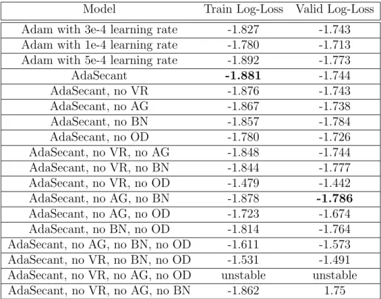
Table 2.1 – Summary of results for the handwriting experiment. We report the best validation log-loss that we found for each model using early stopping. We also report the corresponding train log-loss. In all cases, the log-loss is computed per data point.

(31)

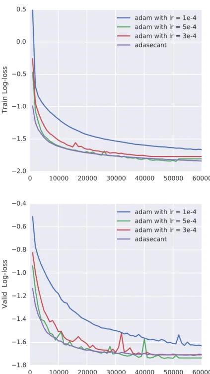
tection (OD). Also, we compared against ADAM ? with different learning rates in Figure 2.1. There, we observe that adasecant performs as well as Adam with a carefully tuned learning rate.

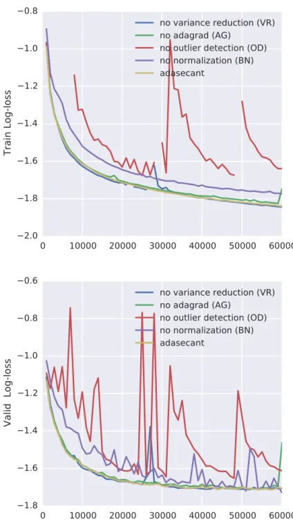
In Figure 2.2, we disable each of the four components of the algorithm. We find that BN provides a small, but constant advantage in performance. OD is also important for the algorithm. Disabling OD makes training more noisy and unstable and gives worse results. Disabling VR also makes training unstable. AG has the least effect in the performance of the algorithm. Furthermore, disabling more than one component makes training even more unstable in the majority of scenarios. A summary of the results is available in Table2.1. In all cases, we use early stopping on the validation log-loss. Furthermore, we present the train log-loss corresponding to the best validation loss as well. Let us note that the log-loss is computed per data point.

2.10.2 PTB Character-level LM

We have run experiments with GRU-RNN? on PTB dataset for character-level language modeling over the subset defined in ?. On this task, we use 400 GRU units with minibatch size of 20. We train the model over the sequences of length 150. For AdaSecant, we have not run any hyperparmeter search, but for Adam we run a hyperparameter search for the learning rate and gradient clipping. The learning rates are sampled from log-uniform distribution between 1e−1 and 6e−5. Gradient clipping threshold is sampled uniformly between 1.2 to 20. We have evaluated 20 different pairs of randomly-sampled learning rates and gradient clipping thresholds. The rest of the hyper-parameters are fixed to their default values. We use the model with the best validation error for Adam. For AdaSecant algorithm, we fix all the hyperparameters to their default values. The learning curves for the both algorithms are shown in Figure 2.3.

2.10.3 MNIST with Maxout Networks

The results are summarized in Figure 2.4 and we show that AdaSecant con-verges as fast or faster than other techniques, including the use of hand-tuned global learning rate and momentum for SGD, RMSprop, and Adagrad. In our experiments with AdaSecant algorithm, adaptive momentum term γk

(32)

at 1.8. In 2-layer Maxout network experiments for SGD-momentum experiments, we used the best hyper-parameters reported by ?, for RMSProp and Adagrad, we crossvalidated learning rate for 15 different learning rates sampled uniformly from the log-space. We crossvalidated 30 different pairs of momentum and learn-ing rate for SGD+momentum, for RMSProp and Adagrad, we crossvalidated 15 different learning rates sampled them from log-space uniformly for deep maxout experiments.

2.11 Conclusion

We described a new stochastic gradient algorithm with adaptive learning rates that is fairly insensitive to the tuning of the hyper-parameters and doesn’t re-quire tuning of learning rates. Furthermore, the variance reduction technique we proposed improves the convergence when the stochastic gradients have high vari-ance. Our algorithm performs as well or better than other popular, carefully-tuned stochastic gradient algorithms. We also present a comprehensive ablation study where we show the effects and importance of each of the elements of our algorithm. As future work, we should try to find theoretical convergence properties of the algorithm to understand it better analytically.

2.12 Appendix

2.12.1 Derivation of Equation

2.18

∂E[(βigi + (1 − βi)E[gi] − gi′)2] ∂βi + λβi2 = 0 E[(βigi + (1 − βi)E[gi] − gi′) ∂(βigi+ (1 − βi)E[gi] − gi′) ∂β ] + λβi = 0

(33)

E[(βigi+ (1 − βi)E[gi] − g′i)(gi− E[gi])] + λβi = 0

E[(βigi(gi− E[gi]) + (1 − βi)E[gi](gi− E[gi])

− g′i(gi− E[gi])] + λβi = 0

βi =

E[(gi− E[gi])(gi′− E[gi])]

E[(gi− E[gi])(gi− E[gi])] + λ

= E[(gi− E[gi])(g

′

i− E[gi])]

Var(gi) + λ

2.12.2 Further Experimental Details

In Figure2.5, we analyzed the effect of using different minibatch sizes for AdaSe-cant and compared its convergence with Adadelta in wall-clock time. For mini-batch size 100 AdaSecant was able to reach the almost same training negative log-likelihood as Adadelta after the same amount of time, but its convergence took much longer. With minibatches of size 500 AdaSecant was able to converge faster in wallclock time to a better local minima.

2.12.3 More decomposition experiments

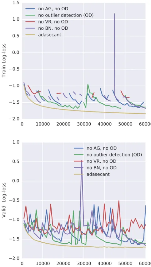
We have run experiments with the different combinations of the components of the algorithm. We show those results on handwriting synthesis with IAM-OnDB dataset. The results can be observed from Figure 2.6, Figure 2.7, Figure2.8, and Figure 2.9 deactivating the components leads to a more unstable training curve in the majority of scenarios.

(34)

0 10000 20000 30000 40000 50000 60000

2.0

1.5

1.0

0.5

0.0

0.5 Train Log-loss

adam with lr = 1e-4

adam with lr = 5e-4

adam with lr = 3e-4

adasecant

0 10000 20000 30000 40000 50000 60000

1.8

1.6

1.4

1.2

1.0

0.8

0.6

0.4 Valid Log-loss

adam with lr = 1e-4

adam with lr = 5e-4

adam with lr = 3e-4

adasecant

Figure 2.1 – Baseline comparison against Adam. AdaSecant performs as well as Adam with a carefully tuned learning rate.

(35)

0 10000 20000 30000 40000 50000 60000

2.0

1.8

1.6

1.4

1.2

1.0

0.8 Train Log-loss

no variance reduction (VR)

no adagrad (AG)

no outlier detection (OD)

no normalization (BN)

adasecant

0 10000 20000 30000 40000 50000 60000

1.8

1.6

1.4

1.2

1.0

0.8

0.6 Valid Log-loss

no variance reduction (VR)

no adagrad (AG)

no outlier detection (OD)

no normalization (BN)

adasecant

Figure 2.2 –Deactivating one component at a time. BN provides a small but constant advantage in performance. OD is important for the algorithm. Deactivating it makes training more noisy and unstable and gives worse results. Deactivating VR also makes training unstable.

(36)

0 20 40 60 80 100 120 140 x400 updates 100 200 300 400 500 600 Cost

Validation learning curve of Adasecant.

Validation learning curve of Adam.

Train learning curve of Adasecant.

Train learning curve of Adam.

Figure 2.3 – Learning curves for the very well-tuned Adam vs AdaSecant algorithm without any hyperparameter tuning. AdaSecant performs very close to the very well-tuned Adam on PTB character-level language modeling task. This shows us the robustness of the algorithm to its hyperparameters. 0 50 100 150 200 250 300 350 # Epochs 10-9 10-8 10-7 10-6 10-5 10-4 10-3 10-2 10-1 100 Train nll (log-scale) Adagrad SGD+momentum Adasecant Rmsprop 0 50 100 150 200 250 300 350 # Epochs 0.0 0.5 1.0 1.5 2.0 2.5 Training nll Adagrad Adasecant SGD+momentum Rmsprop Adadelta

Figure 2.4 – Comparison of different stochastic gradient algorithms on MNIST with Maxout Networks. Both a) and b) are trained with dropout and maximum column norm constraint regularization on the weights. Networks are initialized with weights sampled from a Gaussian distribution with 0 mean and standard deviation of 0.05. In both experiments, the proposed algorithm, Adasecant, seems to be converging faster and arrives to a better minima in training set. We trained both networks for 350 epochs over the training set.

(37)

0 500 1000 1500 2000 2500 3000

Time elapsed for epochs in secs.

10-11 10-10 10-9 10-8 10-7 10-6 10-5 10-4 10-3 10-2 10-1 100 nll in log scale.

Adadelta minibatch size: 100

Adasecant minibatch size: 100

Adasecant minibatch size: 500

Figure 2.5 – In this plot, we compared AdaSecant trained by using minibatch size of 100 and 500 with adadelta using minibatches of size 100. We performed these experiments on MNIST with 2-layer maxout MLP using dropout.

(38)

0 10000 20000 30000 40000 50000 60000 2.0 1.8 1.6 1.4 1.2 1.0 0.8 Train Log-loss no variance reduction (VR) no VR, no OD no VR, no BN no VR, no AG adasecant 0 10000 20000 30000 40000 50000 60000 1.8 1.6 1.4 1.2 1.0 0.8 0.6 0.4 Valid Log-loss no variance reduction (VR) no VR, no OD no VR, no BN no VR, no AG adasecant

(39)

0 10000 20000 30000 40000 50000 60000 2.0 1.8 1.6 1.4 1.2 1.0 0.8 Train Log-loss no adagrad (AG) no AG, no OD no AG, no BN no VR, no AG adasecant 0 10000 20000 30000 40000 50000 60000 1.8 1.6 1.4 1.2 1.0 0.8 0.6 Valid Log-loss no adagrad (AG) no AG, no OD no AG, no BN no VR, no AG adasecant

(40)

0 10000 20000 30000 40000 50000 60000

2.0

1.5

1.0

0.5

0.0

0.5

1.0

1.5 Train Log-loss

no BN, no OD

no AG, no BN

no VR, no BN

no normalization (BN)

adasecant

0 10000 20000 30000 40000 50000 60000

2.0

1.5

1.0

0.5

0.0

0.5

1.0 Valid Log-loss

no BN, no OD

no AG, no BN

no VR, no BN

no normalization (BN)

adasecant

(41)

0 10000 20000 30000 40000 50000 60000 2.0 1.5 1.0 0.5 0.0 0.5 1.0 1.5 Train Log-loss no AG, no OD

no outlier detection (OD) no VR, no OD no BN, no OD adasecant 0 10000 20000 30000 40000 50000 60000 2.0 1.5 1.0 0.5 0.0 0.5 1.0 Valid Log-loss no AG, no OD

no outlier detection (OD) no VR, no OD

no BN, no OD adasecant

(42)

3

_SampleRNN

SampleRNN: An Unconditional End-to-End Neural Audio Genera-tion Model. Soroush Mehri, Kundan Kumar, Ishaan Gulrajani, Rithesh Kumar, Shubham Jain, Jose Sotelo, Aaron Courville, Yoshua Bengio.

Personal Contribution. My main contribution to the project was helping with the analysis of the results. Also, I wrote the code for a conditional version of the SampleRNN model but unfortunately because of the deadline this work was not included in the paper. The model was initially by Ishaan. After, in the Speech Synthesis group, Soroush, Aaron, Yoshua and I discussed this model ex-tensively. Soroush and Kundan rewrote the code and performed and extensive hyper-parameter search. I ran a few experiments reproducing Ishaan’s first results. Later, Soroush wrote most of the paper. I helped analyzing the results and pro-ducing some of the figures in the paper as well as with minor editing of the other sections. This chapter was accepted in the ICLR, 2017.

Affiliations

Soroush Mehri, MILA, Département d’Informatique et de Recherche Opéra-tionnelle, Université de Montréal

Kundan Kumar, Computer Science and Engineering, IIT Kanpur

Ishaan Gulrajani, MILA, Département d’Informatique et de Recherche Opéra-tionnelle, Université de Montréal

Rithesh Kumar, Department of Computer Science and Engineering, Sri Siva-subramaniya Nadar College Of Engineering

Shubham Jain, Department of Computer Science and Engineering, IIT Kanpur Jose Sotelo, MILA, Département d’Informatique et de Recherche Opérationnelle, Université de Montréal

Aaron Courville, MILA, Département d’Informatique et de Recherche Opéra-tionnelle, Université de Montréal, CIFAR Fellow

(43)

Op´era-Funding We acknowledge the support of the following agencies for research funding and computing support: NSERC, Calcul Qu´ebec, Compute Canada, the Canada Research Chairs and CIFAR. This work was a collaboration with Ubisoft.

3.1 Abstract

In this paper we propose a novel model for unconditional audio generation based on generating one audio sample at a time. We show that our model, which profits from combining memory-less modules, namely autoregressive multilayer percep-trons, and stateful recurrent neural networks in a hierarchical structure is able to capture underlying sources of variations in the temporal sequences over very long time spans, on three datasets of different nature. Human evaluation on the gener-ated samples indicate that our model is preferred over competing models. We also show how each component of the model contributes to the exhibited performance.

3.2 Introduction

Audio generation is a challenging task at the core of many problems of interest, such as text-to-speech synthesis, music synthesis and voice conversion. The par-ticular difficulty of audio generation is that there is often a very large discrepancy between the dimensionality of the the raw audio signal and that of the effective semantic-level signal. Consider the task of speech synthesis, where we are typically interested in generating utterances corresponding to full sentences. Even at a rel-atively low sample rate of 16kHz, on average we will have 6,000 samples per word generated.1

Traditionally, the high-dimensionality of raw audio signal is dealt with by first compressing it into spectral or hand-engineered features and defining the genera-tive model over these features. However, when the generated signal is eventually decompressed into audio waveforms, the sample quality is often degraded and re-quires extensive domain-expert corrective measures. This results in complicated

1. Statistics based on the average speaking rate of a set of TED talk speakers http:// sixminutes.dlugan.com/speaking-rate/

(44)

signal processing pipelines that are to adapt to new tasks or domains. Here we propose a step in the direction of replacing these handcrafted systems.

In this work, we investigate the use of recurrent neural networks (RNNs) to model the dependencies in audio data. However, a known problem of these models is that they do not scale well at such a high temporal resolution as is found when generating acoustic signals one sample at a time, e.g., 16000 times per second. This is one of the reasons that ? profits from other neural modules such as one presented by ? to show extremely good performance.

In this paper, an end-to-end unconditional audio synthesis model for raw wave-forms is presented while keeping all the computations tractable.2 _{Since our model}

has different modules operating at different clock-rates (which is in contrast to WaveNet), we have the flexibility in allocating the amount of computational re-sources in modeling different levels of abstraction. In particular, we can potentially allocate very limited resource to the module responsible for sample-level alignments operating at the clock-rate equivalent to sample-rate of the audio, while allocating more resources in modeling dependencies which vary very slowly in audio, for ex-ample, the identity of phonemes being spoken. This advantage makes our model arbitrarily flexible in handling sequential dependencies at multiple levels of abstrac-tion.

Our contribution is threefold:

1. We present a novel method that utilizes RNNs at different scales to model longer term dependencies in audio waveforms while training on short se-quences which results in memory efficiency during training.

2. We extensively explore and compare variants of models achieving the above effect.

3. We study and empirically evaluate the impact of different components of our model on three audio datasets. Human evaluation also has been conducted to test these generative models.

2. Code https://github.com/soroushmehr/sampleRNN_ICLR2017 and samples https:// soundcloud.com/samplernn/sets

(45)

3.3 SampleRNN Model

In this paper we propose SampleRNN (shown in Fig. 3.1), a density model for audio waveforms. SampleRNN models the probability of a sequence of waveform samples X = {x1, x2, . . . , xT} (a random variable over input data sequences) as the

product of the probabilities of each sample conditioned on all previous samples:

p(X) =

T−1

Y

i=0

p(xi+1|x1, . . . , xi) (3.1)

RNNs are commonly used to model sequential data which can be formulated as:

ht= H(ht−1, xi=t) (3.2)

p(xi+1|x1, . . . , xi) = Sof tmax(M LP (ht)) (3.3)

with H being one of the known memory cells, Gated Recurrent Units (GRUs) (?), Long Short Term Memory Units (LSTMs) (?), or their deep variations (Section3.4). However, raw audio signals are challenging to model because they contain structure at very different scales: correlations exist between neighboring samples as well as between ones thousands of samples apart.

SampleRNN helps to address this challenge by using a hierarchy of modules, each operating at a different temporal resolution. The lowest module processes individual samples, and each higher module operates on an increasingly longer timescale and a lower temporal resolution. Each module conditions the module below it, with the lowest module outputting sample-level predictions. The entire hierarchy is trained jointly end-to-end by backpropagation.

3.3.1 Frame-level Modules

Rather than operating on individual samples, the higher-level modules in Sam-pleRNN operate on non-overlapping frames of F S(k) (“Frame Size”) samples at the kth level up in the hierarchy at a time (frames denoted by f(k)_{). Each frame-level}

module is a deep RNN which summarizes the history of its inputs into a condition-ing vector for the next module downward.

(46)

(47)

h(k), H(k)_{, W}(k) j , and r(k). inpt =    Wxft(k)+ c (k+1) t ; 1 < k < K ft(k=K); k = K (3.4) ht = H(ht−1, inpt) (3.5) c(k)_{(t−1)∗r+j} = Wjht; 1 ≤ j ≤ r (3.6)

Our approach of upsampling with r(k) _{linear projections is exactly equivalent to}

upsampling by adding zeros and then applying a linear convolution. This is some-times called “perforated” upsampling in the context of convolutional neural net-works (CNNs). It was first demonstrated to work well in ? and is a fairly common upsampling technique.

3.3.2 Sample-level Module

The lowest module (tier k = 1; Eqs. 3.7–3.9) in the SampleRNN hierarchy out-puts a distribution over a sample xi+1, conditioned on the F S(1) preceding samples

as well as a vector c(k=2)_i from the next higher module which encodes information about the sequence prior to that frame. As F S(1) _{is usually a small value and}

cor-relations in nearby samples are easy to model by a simple memoryless module, we implement it with a multilayer perceptron (MLP) rather than RNN which slightly speeds up the training. Assuming ei represents xi after passing through embedding

layer (section3.3.2), conditional distribution in Eq.3.1can be achieved by following and for further clarity two consecutive sample-level frames are shown. In addition, Wx in Eq. 3.8 is simply used to linearly combine a frame and conditioning vector

from above.

f_i−1(1) = f latten([ei−F S(1), . . . , e_i−1]) (3.7)

fi(1) = f latten([ei−F S(1)₊₁, . . . , e_i])

inp(1)_i = W_x(1)f_i(1)+ c(2)_i (3.8) p(xi+1|x1, . . . , xi) = Sof tmax(M LP (inp(1)i )) (3.9)

We use a Softmax because we found that better results were obtained by dis-cretizing the audio signals (also see ?) and outputting a Multinoulli distribution

(48)

rather than using a Gaussian or Gaussian mixture to represent the conditional density of the original real-valued signal. When processing an audio sequence, the MLP is convolved over the sequence, processing each window of F S(1) _{samples and}

predicting the next sample. At generation time, the MLP is run repeatedly to generate one sample at a time. Table 3.1 shows a considerable gap between the baseline model RNN and this model, suggesting that the proposed hierarchically structured architecture of SampleRNN makes a big difference.

Output Quantization

The sample-level module models its output as a q-way discrete distribution over possible quantized values of xi (that is, the output layer of the MLP is a q-way

Softmax).

To demonstrate the importance of a discrete output distribution, we apply the same architecture on real-valued data by replacing the q-way Softmax with a Gaussian Mixture Models (GMM) output distribution. Table 3.2 shows that our model outperforms an RNN baseline even when both models use real-valued outputs. However, samples from the real-valued model are almost indistinguishable from random noise.

In this work we use linear quantization with q = 256, corresponding to a per-sample bit depth of 8. Unintuitively, we realized that even linearly decreasing the bit depth (resolution of each audio sample) from 16 to 8 can ease the optimization procedure while generated samples still have reasonable quality and are artifact-free.

In addition, early on we noticed that the model can achieve better performance and generation quality when we embed the quantized input values before passing them through the sample-level MLP (see Table 3.4). The embedding steps maps each of the q discrete values to a valued vector embedding. However, real-valued raw samples are still used as input to the higher modules.

Conditionally Independent Sample Outputs

To demonstrate the importance of a sample-level autoregressive module, we try replacing it with “Multi-Softmax” (see Table 3.4), where the prediction of each sample xi depends only on the conditioning vector c from Eq. 3.9. In this

(49)

configu-ration, the model outputs an entire frame of F S(1) _{samples at a time, modeling all}

samples in a frame as conditionally independent of each other. We find that this Multi-Softmax model (which lacks a sample-level autoregressive module) scores sig-nificantly worse in terms of log-likelihood and fails to generate convincing samples. This suggests that modeling the joint distribution of the acoustic samples inside each frame is very important in order to obtain good acoustic generation. We found this to be true even when the frame size is reduced, with best results always with a frame size of 1, i.e., generating only one acoustic sample at a time.

3.3.3 Truncated BPTT

Training recurrent neural networks on long sequences can be very computa-tionally expensive. ? avoid this problem by using a stack of dilated convolutions instead of any recurrent connections. However, when they can be trained effi-ciently, recurrent networks have been shown to be very powerful and expressive sequence models. We enable efficient training of our recurrent model using trun-cated backpropagation through time, splitting each sequence into short subsequences and propagating gradients only to the beginning of each subsequence. We experi-ment with different subsequence lengths and demonstrate that we are able to train our networks, which model very long-term dependencies, despite backpropagating through relatively short subsequences.

Table 3.3 shows that by increasing the subsequence length, performance sub-stantially increases alongside with train-time memory usage and convergence time. Yet it is noteworthy that our best models have been trained on subsequences of length 512, which corresponds to 32 milliseconds, a small fraction of the length of a single a phoneme of human speech while generated samples exhibit longer word-like structures.

Despite the aforementioned fact, this generative model can mimic the existing long-term structure of the data which results in more natural and coherent sam-ples that is preferred by human listeners. (More on this in Sections 3.4.2–3.4.3.) This is due to the fast updates from TBPTT and specialized frame-level modules (Section 3.3.1) with top tiers designed to model a lower resolution of signal while leaving the process of filling the details to lower tiers.

(50)

3.4 Experiments and Results

In this section we are introducing three datasets which have been chosen to evaluate the proposed architecture for modeling raw acoustic sequences. The de-scription of each dataset and their preprocessing is as follows:

Blizzard which is a dataset presented by ? for speech synthesis task, con-tains 315 hours of a single female voice actor in English; however, for our experiments we are using only 20.5 hours. The training/validation/test split is 86%-7%-7%.

Onomatopoeia3_{, a relatively small dataset with 6,738 sequences adding}

up to 3.5 hours, is human vocal sounds like grunting, screaming, panting, heavy breathing, and coughing. Diversity of sound type and the fact that these sounds were recorded from 51 actors and many categories makes it a challenging task. To add to that, this data is extremely unbalanced. The training/validation/test split is 92%-4%-4%.

Music dataset is the collection of all 32 Beethoven’s piano sonatas publicly available on https://archive.org/ amounting to 10 hours of non-vocal audio. The training/validation/test split is 88%-6%-6%.

See Fig.3.2for a visual demonstration of examples from datasets and generated samples. For all the datasets we are using a 16 kHz sample rate and 16 bit depth. For the Blizzard and Music datasets, preprocessing simply amounts to chunking the long audio files into 8 seconds long sequences on which we will perform truncated backpropagation through time. Each sequence in the Onomatopoeia dataset is few seconds long, ranging from 1 to 11 seconds. To train the models on this dataset, zero-padding has been applied to make all the sequences in a mini-batch have the same length and corresponding cost values (for the predictions over the added 0s) would be ignored when computing the gradients.

We particularly explored two gated variants of RNNs—GRUs and LSTMs. For the case of LSTMs, the forget gate bias is initialized with a large positive value of 3, as recommended by ? and ?, which has been shown to be beneficial for learning long-term dependencies.

As for models that take real-valued input, e.g. the RNN-GMM and SampleRNN-GMM (with 4 components), normalization is applied per audio sample with the

Speech synthesis using recurrent neural networks

Résumé

Summary

Contents

List of Figures

List of Tables

List of Abbreviations

1

Introduction

1.1

Machine Learning

1.2

Generative Models

1.4

Neural Networks

1.5

Recurrent Neural Networks

1.6