Viscous stabilizations for high order approximations of Saint-Venant and Boussinesq flows

HAL Id: hal-01361347

https://hal.univ-cotedazur.fr/hal-01361347v2

Submitted on 9 Oct 2016

HAL is a multi-disciplinary open access

archive for the deposit and dissemination of

sci-entific research documents, whether they are

pub-lished or not. The documents may come from

teaching and research institutions in France or

abroad, or from public or private research centers.

L’archive ouverte pluridisciplinaire HAL, est

destinée au dépôt et à la diffusion de documents

scientifiques de niveau recherche, publiés ou non,

émanant des établissements d’enseignement et de

recherche français ou étrangers, des laboratoires

publics ou privés.

Viscous stabilizations for high order approximations of

Saint-Venant and Boussinesq flows

Richard Pasquetti

To cite this version:

Richard Pasquetti. Viscous stabilizations for high order approximations of Saint-Venant and

Boussi-nesq flows. ICOSAHOM 2016, Jun 2016, Rio de Janeiro, Brazil. �hal-01361347v2�

high order approximations of Saint-Venant

and Boussinesq flows

Richard Pasquetti

Abstract Two viscous stabilization methods, namely the spectral vanishing viscos-ity (SVV) technique and the entropy viscosviscos-ity method (EVM), are applied to flows of interest in geophysics. First, following a study restricted to one space dimension [17], the spectral element approximation of the shallow water equations is stabilized using the EVM. Our recent advances are here carefully described. Second, the SVV technique is used for the large-eddy simulation of the spatial and temporal develop-ment of the turbulent wake of a sphere in a stratified fluid [16]. We conclude with a parallel between these two stabilization techniques.

1 Introduction

Simulations of flows that can develop stiff gradients generally suffer from numer-ical instabilities if nothing is done to stabilize the computation. Here we address shallow water flows and the turbulent wake of a sphere in a thermally stratified fluid. Shallow water flows are approximately governed by the Saint-Venant equa-tions, i.e. by a non linear hyperbolic system that can yield shocks depending on the initial conditions. Moreover, one generally expects the numerical scheme to be well balanced and that it can support the presence of dry zones. A large literature is devoted to this questions, see e.g. [1, 22] and references herein. Our simulation of the stratified turbulent wake of a sphere relies on the incompressible Navier-Stokes equations coupled, within the Boussinesq approximation, to an advection-diffusion equation for the temperature. No shocks are in this case expected, but because the smallest scales of the flow cannot be captured by the mesh, here also a stabilization is required. Such a problem is generally addressed using the large-eddy simulation (LES) methodology, see e.g. [18]. In both cases, in the frame of high order methods,

Richard Pasquetti

Universit´e Cˆote d’Azur, CNRS, Inria, LJAD, France, e-mail: richard.pasquetti@unice.fr. Lab. J.A. Dieudonn´e (CASTOR project), Parc Valrose, 06108 Nice Cedex 2.

typically spectrally accurate methods, standard approaches are generally not useful, because implying an unacceptable loss of accuracy.

This paper describes two stabilization techniques that allow, at least formally, to preserve the accuracy of high order methods by introducing relevant viscous terms: The entropy viscosity method (EVM) and the spectral vanishing viscosity (SVV) technique. In Section 2 we develop a spectral element method (SEM) for the Saint-Venant system and we stabilize it using the EVM. In Section 3 we use the SVV technique to carry out a Fourier-Chebyshev large-eddy simulation of the turbulent stratified wake of a sphere, on the basis of stabilized Boussinesq equations. To con-clude, we provide in Section 4 a parallel between these two stabilization techniques.

2 Entropy viscosity stabilized approximation of the Saint-Venant

system

This part follows a previous paper [17] where the one-dimensional (1D) Saint-Venant system was considered and where we especially focused on problems in-volving dry-wet transitions. Here this work is extended to the 2D case. Moreover, the treatment of dry zones is improved and the well balanced feature of the scheme is focused on. Comparisons are done with an analytical solution involving dry-wet transitions and the result of a problem combining shocks with dry zones is presented. The Saint-Venant system results from an approximation of the incompressible Euler equations which assumes that the pressure is hydrostatic and that the pertur-bations of the free surface are small compared to the water height. Then, from the mass and momentum conservation laws and with Ω ⊂ R2for the computational do-main, one obtains equations that describe the evolution of the height h : Ω → R+ and of the horizontal velocity u : Ω → R2: For (x,t) ∈ Ω × R+:

∂th+ ∇ · (hu) = 0 (1)

∂t(hu) + ∇ · (huu + gh2I/2) + gh∇z = 0 (2)

with I, identity tensor, uu ≡ u ⊗ u, g, gravity acceleration, and where z(x) describes the topography, assumed such that ∇z  1. Let us recall the following properties: • The system is nonlinear and hyperbolic, which means that discontinuities may

develop;

• Assuming that the inlet flow-rate equals the outlet flow-rate, the total mass is preserved;

• The height h is non-negative; • Rest solutions are stable;

• There exists a convex entropy (actually the energy E) such that

Set q = hu and let hN(t) (resp. qN(t)) to be the piecewise polynomial continuous

approximation of degree N of h(t) (resp. q(t)). The proposed stabilized SEM relies on the Galerkin approximation of the Saint-Venant system completed with mass and momentum viscous terms. For any vN, wNspanning the same approximation spaces,

in semi-discrete form:

(∂thN+ ∇ · qN, vN)N= −(νh∇hN, ∇vN)N (4)

(∂tqN+ ∇ · IN(qNqN/hN) + ghN∇(hN+ zN), wN)N= −(νq∇qN, ∇wN)N (5)

where νh∝ νq= ν, with ν : entropy viscosity (in the rest of the paper we simply

use νh= νq). The usual SEM approach is used here: INis the piecewise polynomial

interpolation operator, based for each element on the tensorial product of Gauss-Lobatto-Legendre (GLL) points, and (., .)N stands for the SEM approximation of

the L2_{(Ω ) inner product, using for each element the GLL quadrature formula which}

is exact for polynomials of degree less than 2N − 1 in each variable. The following remarks may be expressed:

• Mass conservation is ensured by the present SEM approximation: Set vN = 1

in the equation (4); IfR

ΓqN· dΓ = 0, where Γ is the boundary of Ω , then the

equalities Z Ω (∂thN+ ∇ · qN) dΩ = Z Ω ∂thNdΩ + 0 = dt Z Ω hNdΩ = 0

still hold after the SEM discretization. Note however that it is assumed that the Jacobian determinants of the mappings from the reference element (−1, 1)2to the mesh elements are piecewise polynomials of degree less than N.

• On the contrary, the expected conservation of energy for smooth problems is approximate; This results from the presence of nonlinear terms in (3).

• A stabilization term appears in the mass equation (4). This is required when a high order approximation is involved, i.e. when the scheme numerical diffusion becomes negligible.

• In the momentum equation (5) we do not use the viscous term ∇ · (hν∇u), which turned out to be less efficient. Indeed, for stabilization purposes the physically relevant stabilization may not be the best suited, see e.g. [8] for the Euler equa-tions.

• Thanks to using ∇·IN(gh2NI/2) ≈ ghN∇hN(while h2Nis generally piecewise

poly-nomial of degree greater than N), and thus grouping in (5) the pressure and to-pography terms, a well balanced scheme is obtained by construction: If q_N ≡ 0 and hN6= 0, then hN+ zN= Constant.

• Another difficulty comes from the positivity of hN. This point is addressed at the

end of the present Section.

It remains to define the entropy viscosity ν. To this end we make use of an entropy that does not depend on z but on ∇z, which is of interest, at the discrete level, to get free of the choice of the coordinate system. Taking into account the mass conserva-tion equaconserva-tion one obtains:

∂tE˜+ ∇ · (( ˜E+ gh2/2)u) + ghu · ∇z ≤ 0 , E˜= hu2/2 + gh2/2 . (6)

At each time-step, we then compute the entropy viscosity ν(x) at the GLL grid points, using the following three steps procedure:

• Assuming all variables given at time tn, compute the entropy residual, using a

backward difference formula, e.g. the BDF2 scheme, to approximate ∂tE˜N

rE= ∂tE˜N+ ∇ · IN(( ˜EN+ gh2N/2)qN/hN) + gqN· ∇zN

where ˜EN = q2N/(2hN) + gh2N/2. Then set up a viscosity νEsuch that:

νE= β |rE|δ x2/∆ E ,

where δ x stands for the local GLL grid-size, ∆ E for a reference entropy, and where β is a user defined control parameter.

• Define a viscosity upper bound based on the wave speeds : λ±= u ±

√ gh: νmax= α max Ω (|q_N/hN| + p ghN)δ x

where α is a O(1) user defined parameter (recall that for the advection equation α = 1/2 is well suited).

• Compute the entropy viscosity:

ν = min(νmax, νE)

and smooth: (i) locally (in each element), e.g. in 1D: (νi−1+ 2νi+ νi+1)/4 →

νi; (ii) globally, by projection onto the space of the C0piecewise polynomials

of degree N. Note that operation (ii) is cheap because the SEM mass matrix is diagonal.

The positivity of h is difficult to enforce as soon as N > 1, so that for problems involving dry-wet transitions the present EVM methodology must be completed. The algorithm that we propose is the following: In dry zones, i.e. for any element Qdry such that at one GLL point min hN < hthresh, where hthresh is a user defined

threshold value (typically a thousandth of the reference height):

• Modify the entropy viscosity technique, by using in Q_drythe upper bound first order viscosity:

ν = νmax in Qdry

• In the momentum equation assume that:

hNg∇(hN+ zN) ≡ 0 in Qdry

• Moreover, notice that the upper bound viscosity νmaxis not local but global, and

that the entropy scaling ∆ E used in the definition of νEis time independent. This

The numerical results presented hereafter have been obtained using the standard SEM for the discretization in space (GLL nodes for interpolations and quadratures) and the usual forth order Runge-Kutta (RK4) scheme for the discretization in time. To outline the efficiency of the present EVM for stabilization of Saint-Venant flows involving dry-wet transitions, we first consider a problem for which an an-alytical solution is available: The planar fluid surface oscillations in a paraboloid [21]. The topography is defined by z(x) = D0x2/L2and the exact solution is given

by: h= max(0, 2ηD0 L ( x1 L cos(ωt) − x2 L sin(ωt) − η 2L) + D0− z) u = −ηω(sin(ωt) , cos(ωt))

where η determines the amplitude of the motion and with ω =√2gD0/L. Here we

use L = 1 m, D0= 0.1 m and η = 0.5 m.

Fig. 1 Planar oscillations in a paraboloid: Error on the height and at the final time for the first order viscosity (left) and EVM (right) solutions.

The computational domain is a circle centered at the origin and of diame-ter 4. The discretization paramediame-ters are the following, number of elements: 2352, polynomial approximation degree: N = 5, resulting number of grid-points: 59081, time-step: 2.96 10−4 , EVM control parameters: α = 1, β /∆ E = 10. Moreover, hthresh = maxΩh0/500, with h0≡ h(t = 0), and at the initial time one sets hN =

IN(max(h0, hthresh/2)). Since here the exact solution is only C0continuous, the

com-putation cannot be spectrally accurate and so the convergence rate would be disap-pointing. This is why, in order to outline the interest of using a high order method like the present stabilized SEM, we prefer to compare the EVM results to results obtained with a first order viscosity. One looks in Fig. 1 at the error |hN− h|(x)

at time t ≈ 6π/ω, i.e. after three loops of the fluid surface inside the paraboloid. Fig. 1 (left) gives this error field when using the first order viscosity, that is with νh= νq= νmax, whereas Fig. 1 (right) shows the result obtained when using the

viscosity for stabilization yields a result by far worse than the one obtained with the EVM. Animations of these error fields clearly confirm such a conclusion. An-other test case provided in [21] has also been investigated, namely the axisymmetric oscillations in a paraboloid, and the conclusion is quite similar.

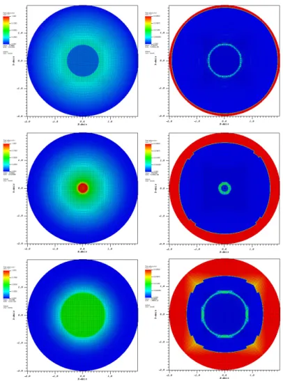
Fig. 2 Axisymmetric oscillations with shocks in a paraboloid: Height (left) and entropy viscosity (right), at t ≈ 1.4 (top), t ≈ 1.65 (middle) and t ≈ 1.9 (bottom).

To conclude this Section we give the results of a simulation that shows axisym-metric oscillations in a paraboloid and that involves both dry-wet transitions and shocks. The initial condition is the following:

and at the boundary an impermeability condition together with an homogeneous Neumann condition for h are imposed. The geometry and the space discretization are those used in the first example. Calculations have been made till time t = 5 with time-step 10−4, and the EVM control parameters are: α = 1, β /∆ E = 20. As pre-viously, h_thresh= maxΩh0/500 and at the initial time hN = IN(max(h0, hthresh/2)).

Such a flow is alternatively expanding and then retracting towards the paraboloid axis. Fig. 2 shows the flow at three different times, during the first retraction-expansion phase: At t ≈ 1.4 the velocity field is inwards, at t ≈ 1.65 it is close to reversal and at t ≈ 1.9 it is outwards. The height hN (at left) and the entropy

vis-cosity ν (at right) are visualized. As desired, the entropy visvis-cosity saturates in dry zones and also focuses at the shock.

3 Spectral vanishing viscosity for large-eddy simulation of the

stratified wake of a sphere

To demonstrate the interest of using the SVV technique for the computation of tur-bulent flows, we consider the turtur-bulent wake of a sphere in a thermally stratified fluid. Here we just focus on the main characteristics of the SVV technique and il-lustrate its capabilities for this particular geophysical flow. Details concerning the physical study may be found in [16].

The SVV technique was initially developed to solve with spectral methods (Fourier / Legendre expansions) hyperbolic problems (non-linear, scalar, 1D, typ-ically the Burgers equation), while (i) preserving the spectral accuracy and (ii) pro-viding a stable scheme [13, 20]. Later on, say in the 2000’s, the SVV technique turned out to be of interest for stabilization of the Navier-Stokes equations and so for the large-eddy simulation (LES) of turbulent flows, see e.g. [10, 11, 12, 14, 15, 23] and references herein.

The basic idea of the SVV stabilization technique is to add some artificial viscos-ity on the highest frequencies, i.e., to complete the conservation law of some given quantity u, assumed to be scalar for the sake of simplicity, with the SVV term :

VN≡ εN∇ · (QN(∇uN))

where N is again the polynomial degree, uN the numerical approximation of u, εN

a O(1/N) coefficient and QN the so-called spectral viscosity operator, defined to

select the highest frequencies: If QN is omitted in the definition of VN, then one

recovers a first order viscosity term.

In spectral space (Fourier, Chebyshev, Legendre, or any other hierarchical basis) the operator QN is defined by a set of coefficients bQk, 0 ≤ k ≤ N. Thus, in the 1D

periodic case and if Fourier expansions are concerned (trigonometric polynomials are involved in this case):

with (_b.)_k for the k-Fourier component, (.) for complex conjugate, and where the coefficients bQ_k are such that bQ_k= 0 for k ≤ mN, with mN a threshold value, and

0 < bQk≤ 1 , bQkbeing monotonically increasing, for k > mN. In the seminal paper

[20], bQkwas simply chosen as a step function, i.e. with bQk= 1 if k > mN, but it

quickly appeared of interest to rather use a smooth approximation. In Fig. 3 two SVV kernels are shown, using the smooth approximation proposed in [13] and with mN= N/2 and mN= N/4. 0 0.2 0.4 0.6 0.8 1 0 0.2 0.4 0.6 0.8 1 Qk k / N Spectral viscosity operator m/N=0.25

m/N=0.5 C-L HV-2

Fig. 3 bQkfor two SVV kernels, and if using an hyperviscosity (HV) or the Chollet-Lesieur (C-L)

subgrid scale model.

One may remark that if defining differently the bQk coefficients, one recovers

alternative approaches. Thus, the hyperviscosity stabilization, i.e. such that VN ∝

−∆2_u

N, so that (bVN)k∝ k4(ubN)k, can be recasted in the SVV frame by stating that b

Qk= (k/N)2. In this case, the interpolating curve bQk(k) is simply a parabola, see

Fig. 3. Also, if choosing εN ∝ N−4/3 and with the curve bQk(k) shown in Fig. 3,

one recovers the Chollet-Lesieur spectral viscosity [3], developed for LES in the early 80’s and based on the Eddy Damped Quasi-Normal Markovian (EDQNM) theory. This latter approach strongly differs from SVV, since bQk6= 0 even for k =

0, but both approaches also differ from SVV because the associated kernels no-longer constitute an approximation of a step function. As a result, it is no no-longer a Laplacean which is acting in the high frequency range. Indeed, if the SVV kernel is simply a step function, then the stabilization term also writes VN= εN∆ uH_N, where uH

N is the high frequency part of uN.

Results obtained with a multi-domain spectral Chebyshev-Fourier solver with SVV stabilization are presented hereafter, see [16] for details. The turbulent wake is generated by a sphere moving horizontally and at constant velocity in a stably strat-ified fluid, with constant temperature gradient. The flow is assumed governed by the Boussinesq equations and the control parameters are Pr = 7, Re = 10000, F = 25, for the Prandtl, Reynolds and internal Froude number, respectively. The study is car-ried out in two steps: First we make a space development study, that is the Galilean

Fig. 4 Temperature field in the median vertical plane at the end of the space development study (color scale: −4 to 4, from blue to red) [16].

frame is associated to the moving sphere; Second, we make a time development study, with a Galilean frame at rest. Such an approach is required to compute the far wake without needing a very elongated computational domain. With respect to anterior works, see e.g. [4, 5], the originality of the present study is to make use of the result of the space development study for setting up the initial condition of the temporal development study, thus avoiding the use of a synthetic initial condition.

For the space development study, the computational domain is (−4.5, 30.5) × (−4, 4) × (−4, 4). At the initial time, the fluid is stably stratified: T0= y. The sphere,

of unit diameter and centered at (0, 0), is modeled by using a volume penalization technique. For the boundary conditions one has: Dirichlet conditions at the inlet, advection at the mean velocity at the outlet, free-slip / adiabaticity conditions on the upper and lower boundaries. The mesh makes use of 12.4 106grid-points. For the velocity components, the SVV parameters are: mN = N/2, εN = 1/N, where

N is here associated to each of the three axis, whereas for the temperature, mN =

√

N, εN= 1/N. The temperature field obtained at the end of the space development

study is shown in Fig. 4

Fig. 5 Temperature and vorticity fields at the beginning (left panel) and at the end (right panel) of the temporal development study. Up: Temperature in the median vertical plane; Middle: Transverse component of the vorticity in the same plane; Bottom: vertical component in the median horizontal plane. The vorticity being much weaker at the final time, the vorticity color scales differ [16].

For the temporal development study the computational domain is (−18, 18) × (−4, 4) × (−12, 12). Note it has been enlarged, since we expect, from the confine-ment effect due to the stratification, a strong expansion of the wake in the horizontal plane. The initial conditions are set up from the spatial development study, by ex-traction of the fields obtained at the final time in (6.5, 24.5) × (−4, 4) × (−4, 4). The boundary conditions are: periodicity in streamwise direction, free-slip and adi-abaticity elsewhere. The mesh makes use of 27.7 106grid-points. The SVV parame-ters have not been changed. The flow, at the beginning and at the end of the temporal study, is visualized in Fig. 5.

1 10 1 10 100 Wake amplitude Time (N t) mean half-width mean half-height (N t)**1/3 1 1 10 100 Velocity defect x F 2/3 Time (N t) max u exp.

Fig. 6 Wake amplitude (left) and velocity deficit (right) vs time (N, buoyancy angular frequency) [16].

We conclude with some more quantitative results: In Fig. 6-left one has the evolu-tion of the wake amplitude, both in the vertical and horizontal planes, which clearly points out the confinement effect of the stratification (here Nt is a dimensionless time, with N buoyancy angular frequency); Fig. 6-right shows the evolution of the velocity defect. This latter curve is in reasonable agreement with the “universal curve” of [19], where three phases in the development of sphere stratified wakes are described: First the 3D phase, then the non equilibrium (NEQ) phase and finally the quasi two 2D (Q2D) phase. Tab. 7 compares the experimental results to the present numerical ones, in terms of characteristic quantities of the velocity defect evolution.

NtI NtII 3D rate NEQ rate Q2D rate

[19] 1.7 ± 0.3 50 ± 15 −2/3 −0.25 ± 0.4 −0.76 ± 0.12 SVV-LES 2.4 30 ∼ −2/3 −0.2 ∼ −0.76

Fig. 7 Critical times NtIand NtIIthat correspond to the 3D-NEQ and NEQ-Q2D transitions,

4 Concluding parallel between the EVM and SVV stabilizations

Two viscous stabilizations, namely the entropy viscosity method (EVM) and the spectral vanishing viscosity (SVV) technique, have been successfully implemented in high order approximations of geophysical flows: With EVM shallow water flows involving dry-wet transitions have been addressed and with SVV the turbulent wake of a sphere in a thermally stratified fluid has been investigated. We conclude with a parallel between these two approaches:

• Both SVV and EVM are viscosity methods first developed for hyperbolic prob-lems, see [6, 20].

• EVM is non-linear while SVV is linear. SVV is thus not costly, since its imple-mentation is done in preprocessing step. Moreover, because of this linear feature it is very robust and so well adapted to the LES of turbulent flows.

• Both EVM and SVV preserve the accuracy of the numerical approximation. This is of course essential when high order methods are concerned.

• SVV is not Total Variation Diminishing (TVD) and EVM is not fully TVD, since this depends on the values of the EVM control parameters (α and β ). For SVV, a post processing stage for removing spurious oscillations has been suggested [13]. • A theory exists for SVV [20], whereas no complete theory is available for EVM. Some theoretical results, restricted to some specific time schemes and space ap-proximations, are however available [2].

• EVM may be used with various numerical methods, since based on a physical argument, including the standard finite element method (FEM), finite volume methods etc.. SVV is restricted to spectral type methods, e.g. high order FEMs like the SEM.

• SVV has proved to be of interest for LES (SVV-LES). Preliminary numerical experiments are now available for EVM [9], but additional tests and comparisons remain needed to check if EVM is not too diffusive and robust enough when turbulent flows are concerned.

Acknowledgements Part of this work was made at the Dpt of Mathematics of National Taiwan University in the frame of the Inria project AMOSS.

References

1. C. Berthon, F. Marche, A positive preserving high order VFRoe scheme for shallow water equations: a class of relaxation schemes, SIAM J. Sci. Comput., 30, 2587-2612, 2008. 2. A. Bonito, J.L. Guermond, B. Popov, Stability analysis of explicit entropy viscosity methods

for non-linear scalar conservation equations, Math. Comp., 83, 1039-1062, 2014.

3. J. P. Chollet, M. Lesieur, Parametrisation of small scales of three-dimensional isotropic tur-bulence utilizing spectral closures, J. of Atmospheric Sciences, 38, 2747-2757, 1981. 4. P.J. Diamessis, J.A. Domaradzki, J.S. Hesthaven, A spectral multidomain penalty method

model for the simulation of high Reynolds number localized incompressible stratified turbu-lence, J. Comput. Phys., 202, 298-322, 2005.

5. D.G. Dommermuth, J.W. Rottman, G.E. Innis, E.V. Novikov, Numerical simulation of the wake of a towed sphere in a weakly stratified fluid, J. Fluid Mech., 473, 83-101, 2002. 6. J.L. Guermond, R. Pasquetti, Entropy-based nonlinear viscosity for Fourier approximations

of conservation laws, C.R. Acad. Sci. Paris, Ser. I, 346, 801-806, 2008.

7. J.L. Guermond, R. Pasquetti, B. Popov, Entropy viscosity method for non-linear conservation laws, J. of Comput. Phys., 230 (11), 4248-4267, 2011.

8. J.L. Guermond, B. Popov, Viscous regularization of the Euler equations and entropy princi-ples, SIAM J. Appl. Math., 74 (2), 284-305, 2014.

9. J.-L. Guermond, A. Larios, T. Thompson, Validation of an entropy-viscosity model for large eddy simulation, Direct and Large Eddy-Eddy Simulation IX, ECOFTAC Series, Vol. 20, 43-48, 2015.

10. G. S. Karamanos, G. E. Karniadakis, A spectral vanishing viscosity method for large-eddy simulation, J. Comput. Phys., 163, 22-50, 2000.

11. R. M. Kirby, S. J. Sherwin, Stabilisation of spectral / hp element methods through spectral vanishing viscosity: Application to fluid mechanics, Comput. Methods Appl. Mech. Engrg., 195, 3128–3144, 2006.

12. K. Koal, J. Stiller, H.M. Blackburn, Adapting the spectral vanishing viscosity method for large-eddy simulations in cylindrical configurations, J. of Comput. Phys., 231, 3389-3405, 2012.

13. Y. Maday, S. M. O. Kaber, E. Tadmor, Legendre pseudo-spectral viscosity method for non-linear conservation laws, SIAM J. Numer. Anal., 30, 321-342, 1993.

14. R. Pasquetti, Spectral vanishing viscosity method for large-eddy simulation of turbulent flows, J. Sci. Comp., 27, 365-375, 2006.

15. R. Pasquetti, E. S´everac, E. Serre, P. Bontoux, M. Sch¨afer, From stratified wakes to rotor-stator flows by an SVVLES method, Theor. Comput. Fluid Dyn., 22, 261-273, 2008. 16. R. Pasquetti, Temporal / spatial simulation of the stratified far wake of a sphere, Computers

& Fluids, 40, 179-187, 2010.

17. R. Pasquetti, J.L. Guermond, B. Popov, Stabilized spectral element approximation of the Saint-Venant system using the entropy viscosity technique, in Lecture Notes in computa-tional Science and Engineering : Spectral and High Order Methods for Partial Differential Equations - ICOSAHOM 2014, vol. 106, Springer, 397-404, 2015.

18. P. Sagaut, Large Eddy Simulation for Incompressible Flows, Springer Berlin Heidelberg, 2006.

19. G.R. Spedding, F.K. Browand, A.M. Fincham, The evolution of initially turbulent bluff-body wakes at high internal Froude number, J. Fluid Mech., 337, 283-301, 1997.

20. E. Tadmor, Convergence of spectral methods for nonlinear conservation laws, SIAM J. Numer. Anal., 26, 30-44, 1989.

21. W.C. Thacker, Some exact solutions to the nonlinear shallow-water wave equations, J. Fluid Mech., 107, 499-508, 1981.

22. Y. Xing, X. Zhang, Positivity-preserving well-balanced discontinuous Galerkin methods for the shallow water equations on unstructured triangular meshes, J. Sci. Comput., 57, 19-41, 2013.

23. C.J. Xu, R. Pasquetti, Stabilized spectral element computations of high Reynolds number incompressible flows, J. Comput. Phys., 196, 680-704, 2004.