Revisiting absolute gravimeter intercomparisons

HAL Id: hal-01087247

https://hal.archives-ouvertes.fr/hal-01087247

Submitted on 25 Nov 2014

HAL is a multi-disciplinary open access archive for the deposit and dissemination of sci-entific research documents, whether they are pub-lished or not. The documents may come from teaching and research institutions in France or abroad, or from public or private research centers.

L’archive ouverte pluridisciplinaire HAL, est destinée au dépôt et à la diffusion de documents scientifiques de niveau recherche, publiés ou non, émanant des établissements d’enseignement et de recherche français ou étrangers, des laboratoires publics ou privés.

O de Viron, M van Camp, O Francis

To cite this version:

O de Viron, M van Camp, O Francis. Revisiting absolute gravimeter intercomparisons. Metrologia, IOP Publishing, 2011, 48, pp.290 - 298. �10.1088/0026-1394/48/5/008�. �hal-01087247�

O. de Viron1

, M. Van Camp1,2_{, O. Francis}3

1

Univ. Paris Diderot, Sorbonne Paris Cit´e, Institut de Physique du Globe de Paris,F-75013 Paris, France.

2

Royal Observatory of Belgium, Brussels, Belgium

3

University of Luxembourg, Luxembourg. E-mail: [email protected]

Abstract. Absolute gravimeter allows to determine the local value of gravity, which makes challenging its accuracy assessment. The instrumental offsets are classically estimated by performing comparisons of the results obtained by a set of instruments measuring at the same location but at different epochs (measuring at the same place and epoch is physically impossible). Such intercomparison campaigns have been done a few times since 1980. In this paper, we discuss the method of data processing used for those comparisons. We demonstrate that one of the methods used is inadequate, as it underestimates the dispersion of the instrumental offsets, which is the only reliable quantity that can be obtained from such a comparison. We also propose a new criterion, based on the minimization of the L1 norm of the offsets, for fixing the constant of the ill-conditioned problem, which we show to be statistically more precise than the one classically used.

1. Introduction

Measuring gravity is a challenging task, as it requires to measure very small deviations of a strong acceleration. During the 80ies, with the improvement of measurement techniques, it became possible to build ballistic absolute gravimeters, which determine

the absolute value of the gravity acceleration with a precision of 10−9_{at a given place and}

time [1]. Such a level of precision is necessary to investigate geodynamic phenomena and for high precision metrological experiments aiming at the new definition of the kilogram, for instance [2].

There is no other measurement principle which has a smaller combined standard uncertainty than the ballistic asolute gravimeters considered here, which makes it difficult to assess how accurate they are. The only possible way to estimate their accuracy is to compare them to each other on a regular basis. Since 1980, 8 International Comparisons of Absolute Gravimeters (ICAG) were organized at the Bureau International des Poids et Mesures (BIPM) [3, and references therein]. The objectives are: (1) to determine the level of uncertainty in the absolute measurements of the gravity and (2) to determine a comparison reference value (CRV) for g at the sites of the BIPM gravity network. Moreover, during the ICAGs, relative spring gravimeters participated in the determination of the vertical gravity gradient and, since 2001, of the gravity differences between the different sites. Results including relative gravimeters in the determination of the comparison reference value have been presented for the first time in the ICAG-2001 report [4]. Originally, given the small number of absolute gravimeters, this was done to improve the precision of the transfer in gravity between the sites, mandatory for comparing the gravity from the different sites at the BIPM [4]. Since 2003, two regional comparisons of absolute gravimeters were organized at the Underground Laboratory for Geodynamics in Walferdange (WULG)[5,6]; another one will be organized in November 2011. Those aim at determining the offsets between the absolute gravimeters, but they differ from the ICAG as they do not estimate the CRV. The relative gravimeters do not participate in these comparisons; they were only used to determine the vertical gravity gradients [5].

The comparison requires all the instruments to measure at exactly the same location, which is of course physically impossible simultaneously. Consequently, the comparison is done with instruments measuring the gravity at common locations but at different epochs. During the last comparisons, the time variable part of the signal has been monitored either by the absolute gravimeter measuring during comparisons always at the same location or by a superconducting gravimeter. The observed changes in the gravity residuals, after correcting for tidal and atmospheric pressure effects, were below 1 microgal due to favorable meteorological conditions (Heavy rains may indeed induce gravity changes of a few microgal in less than an hour). No corrections have been applied as the gravity changes were small enough to be ignored.

instrument measure everywhere or at a same location provided that enough data is collected to solve for all the unknowns, i.e. the offset of each instrument and the gravity at each location. During the WULG campaigns, given that 15 sites are available, work is planned in such a way that (1) each instrument measures at least three sites, (2) each site is visited by at least three instruments, and (3) two different instruments, which occupied the same site, did not measure at another common site again. Those conditions allow a better conditioning of the equation system.

Prior 2001, for the ICAG campaigns, gravity was calculated at each site by averaging the gravity value coming from each absolute gravimeter that measured at that site. If a same gravimeter measured more than one time at the same site, each gravity value was first averaged before contributing to the general average. Then, at each site and for each gravimeter, the offsets were determined. Finally, the offsets obtained for each instrument are averaged, giving the final value of the offset of the absolute gravimeter. For details on the combined adjustment of absolute and relative gravimeter to transfer the g values at the CRV site see e.g. [4].

From the ICAG 2001 [3, 8], a least-square adjustment of both relative and absolute gravimeter measurements was performed, where each absolute gravity measurement is modeled as the sum of the value of the gravity at the site, the instrumental offset and the measurement error. Francis et al. [6] compared this method, referenced as ”OF” in that paper and ”Method 2” in this work, to the average method applied for the ICAGs before 2001 (referenced as ”AG” in [6] and as ”Method 1” in this paper). They evidenced slightly more dispersed offsets when using Method 2. However, neither this paper nor ICAG-related publication does further investigate the reason of this dispersion.

The present paper demonstrates that Method 1 provides incorrect estimates of the offsets, underestimating the dispersion of the gravimeter offsets. Based on a simple example (3 gravimeters measuring at 3 sites) and a more realistic one (18 gravimeters and 12 sites) with no measurement errors, we show that Method 1 provides erroneous results even in the framework of its own hypotheses, whereas the Method 2 finds the right values. Classically, Method 2 hypothesizes that the average offset is zero, in order to prevent the equation system from being undetermined. We show in this paper that this method is highly sensitive to outliers, and that better results can be obtained by imposing a zero median. This is physically sounded, as it is equivalent to chose the shift so that the L1-norm of the offsets (i.e. the sum of the absolute values of the individual offsets) is minimal, which makes sense for metrological instruments such as absolute gravimeters.

A second part of this paper consists in comparing the methods on actual measurements. We selected two campaigns: the ICAG 2005, as results were published with and without incorporating the relative gravimeters, and the WULG 2007 regional comparison, as, for the first time, the results from the average Method 1 and the least squares Method 2 were both published.

For the evaluation of comparison data, it is often referred to the procedures described by Cox [8]. He proposed guidelines for two procedures that could be used

to evaluate key comparison data. Unfortunately, these procedures treat only the cases for which all the involved apparatus measure the same quantity resulting in one unique value. As previously explained, during a comparison of absolute gravimeters, several sites with different gravity values are used for practical reasons. The Cox’s procedures cannot be apply directly as they require to transfer all the data to one reference site that will serve as the CRV. The drawback is that this transfer (for which the gravity ties have to be measured) will increase the uncertainty budget. Due to the specificity of the AG comparisons, we propose a third procedure in which the offsets of each gravimeter and the g values at the different sites are estimated directly from the observations avoiding the passage by a unique CRV. This approach is not new. This is what is basically done in Methods 1 and 2.

After the pilote studies, a first Key comparison was performed in 2009. We strongly believe that the procedure for the evaluation of the data of the absolute gravimeter key comparisons needs to be defined and agreed upon. This present paper is our contribution to reach this objective.

2. Resolution Techniques

In an ideal world, an absolute gravimeter comparison experiment would be an easy thing. We would have a standard gravity, known to a precision much better than what AG can provide, and we would simply compare the measurement with the standard. The problem is that there is no such thing as a “perfect” instrument, to which the others could be compared. Consequently, the instruments can only be compared to each other, hoping that, somehow, they are correct in average. Looking how well the AGs are doing in the measurement of g is also a way to evidence systematic errors in the instrument, the measurement method or in the data processing, if the dispersion of the results is larger than the declared uncertainties.

In a less perfect but fairly good world, we could put all the instruments at the same place, so that we could simply compare them all to each other. Unfortunately, the spatial variation of gravity would require the instrument to be exactly at the same place, which is physically impossible. In addition, in the real world, the gravity changes with time, but this is something well known, especially if some absolute or relative gravimeters are continuously measuring during the comparison campaign. So we can correct for that, in such a way that we can compare instruments that have been at the same location at different epochs [6, 8].

The intercomparison consists in having N instruments that have measured at some of the M available locations, with at least 2 measurements by instrument and by site; from this information, we want to determine the individual absolute offsets, and possibly the gravity at each site.

According to Method 1, the average value of all the measurement at each site is a fair estimate of the gravity at this site. So, the difference between each individual measurement and this average value is an independent measurement of the instrumental

offset. Consequently, model is based on the equation (1) here below: gij− ¯g j = δi+ ǫ j i (1)

where g_ij is the measurement value obtained at site j by instrument i, ¯gj _{is the average}

of all the gravity values measured at site j, δi is the offset of instrument i, and ǫji is the

measurement error for the measure gj_i.

The Method 2 is conceptually more straightforward. It is based on a normal equation saying that the gravity value obtained by instrument i at site j is equal to the sum of the gravity at site j plus the offset of instrument i and the measurement error:

g_ij = gj_{+ δ}

i+ ǫ

j

i (2)

The two methods would then be solved by a least square fit, which becomes a simple mean in Method 1. On the other hand, Method 2 has a huge problem: the system is ill-conditioned, because a true value of a quantity is by nature indeterminate. In other words, measurements will be exactly the same for any given number added to all the offsets and subtracted from all the gravity values.

In order to get a solution, we need to add one equation that prevents the system to be ill-conditioned. Many solutions can be proposed. For example, we can take one instrument as exact, with a zero offset, we can consider that the average offset is zero, or we can impose a subset of offsets to have a zero mean. As the model being exact is one of the major assumptions of the least square methods, it is not a trivial action, but we are left with no other choice.

At this point, the Method 1 could seem more appealing, as no such additional equation is required, but this is not true. Actually, Method 1 uses one similar assumption by observation site (the average of the measurements at the site is the true gravity), which makes it more dangerous than Method 2.

3. Simulations

3.1. Case of three gravimeters

3.1.1. Method 1 Let us suppose three absolute gravimeters G1, G2, G3, each measuring

at two sites out of three (A,B,C). Let us write again gj _{the gravity at site j and δ}

i the

offset of instrument i. Let us also suppose for now that there is no measurement error. The equation system of Method 1 becomes:

gA 1 − gA 1 + g3A 2 = δ ′ 1 g1B− gB 1 + g2B 2 = δ ′′ 1 g2B− gB 1 + g2B 2 = δ ′ 2 (3)

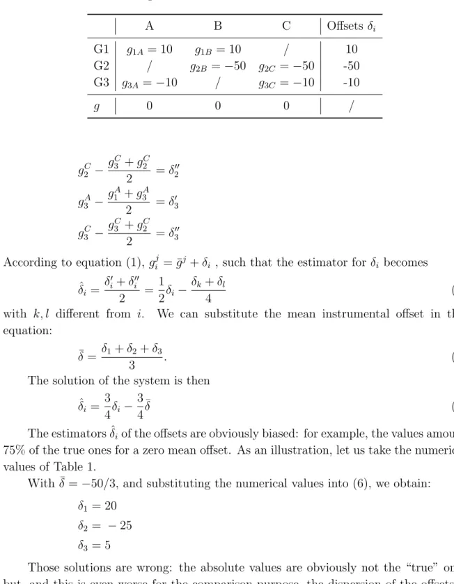
Table 1. Numerical values for a simple case (all in µGal). The line g gives the “true” gravity values, the column offsets gives the “true” offsets, and the values giX are the

simulated observations. As we work in an idealistic errorless case, the values are simply the sum of the g value of the column and the offset value of the line.

A B C Offsets δi G1 g1A = 10 g1B = 10 / 10 G2 / g2B = −50 g2C = −50 -50 G3 g3A = −10 / g3C = −10 -10 g 0 0 0 / g2C− gC 3 + gC2 2 = δ ′′ 2 g3A− gA 1 + g3A 2 = δ ′ 3 g3C− gC 3 + gC2 2 = δ ′′ 3 According to equation (1), g_ij = ¯gj _{+ δ}

i , such that the estimator for δi becomes

ˆ δi = δ′ i+ δi′′ 2 = 1 2δi− δk+ δl 4 (4)

with k, l different from i. We can substitute the mean instrumental offset in this equation:

¯

δ = δ1+ δ2+ δ3

3 . (5)

The solution of the system is then ˆ δi = 3 4δi− 3 4¯δ (6)

The estimators ˆδiof the offsets are obviously biased: for example, the values amount

75% of the true ones for a zero mean offset. As an illustration, let us take the numerical values of Table 1.

With ¯δ = −50/3, and substituting the numerical values into (6), we obtain:

δ1 = 20

δ2 = − 25

δ3 = 5

Those solutions are wrong: the absolute values are obviously not the “true” ones but, and this is even worse for the comparison purpose, the dispersion of the offsets is underestimated by about 25%. This can be explained simply. The offset values are the mean of the offset obtained at each site. When comparing G2 and G3 at the site C – both with a negative offset, we found a mean value which is deviated to the negative

values (equal to -30 rather than zero). The two offsets are then determined at site C using wrong gravity values: -20µGal for G2 (very optimistic) and 20µGal for G3 (pessimistic), which eventually affects the retrieved offsets.

3.1.2. Method 2 In this simple case, the equation system reads:

g1A = g A + δ1 gA 3 = g A_{+ δ} 3 g1B = g B + δ1 (7) gB 2 = g B_{+ δ} 2 gC 2 = g C _{+ δ} 2 g3C = g C + δ3

We add the following equation, to solve the ill-conditioning of the problem:

δ1+ δ2+ δ3

3 = ¯δ = 0µGal. (8)

As the observation system only allows solving for the unknown within an additive constant, we have to add an absolute constrain like equation (8). In our synthetic case, we know that equation (8) is false, and that the equation (9) here below would be more appropriate

δ1+ δ2+ δ3

3 = ¯δ = −

50

3 µGal. (9)

Unfortunately, in the real world, the true value of the mean offset is unknown, so we have to guess the absolute information. Many other options could be chosen, for instance only one of the offsets could be imposed to be zero, but probabilistically, the variance of the mean is lower than the variance of the individual values, which makes the expected error smaller. The absolute value obtained from the experience will only be as good as this information we have guessed. The analytic solution of the system for the error free problem is

ˆ

gX _{= g}X _{+ ¯δ}

ˆ

δi = δi− ¯δ

(10)

Note that, as long as the absolute information is exact, i.e. ¯δ = 0µGal, the estimates of

the gravity values and of the offsets are exact. Using the numerical values of Table 1, we found the following numerical values:

δ1 = 80 3 µGal δ2 = − 100 3 µGal δ3 = 20 3 µGal

In this synthetic case, we know the true value of the offset, so we can compare our estimate with the reality. We found offset estimates that are shifted by -50/3µGal=-16.7µGal from their true value, i.e. exactly the error we did on our absolute information

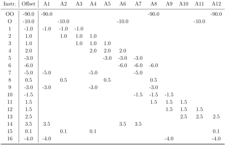
Table 2. Numerical values in a realistic case (all in µGal). The gravity value has been set to 0 everywhere, the column offset gives the “true” offset, and the values are the simulated observations. As we work in an idealistic errorless case, the values are simply the value of the instrumental offsets.

Instr. Offset A1 A2 A3 A4 A5 A6 A7 A8 A9 A10 A11 A12

OO -90.0 -90.0 -90.0 -90.0 O -10.0 -10.0 -10.0 -10.0 1 -1.0 -1.0 -1.0 -1.0 2 1.0 1.0 1.0 1.0 3 1.0 1.0 1.0 1.0 4 2.0 2.0 2.0 2.0 5 -3.0 -3.0 -3.0 -3.0 6 -6.0 -6.0 -6.0 -6.0 7 -5.0 -5.0 -5.0 -5.0 8 0.5 0.5 0.5 0.5 9 -3.0 -3.0 -3.0 -3.0 10 -1.5 -1.5 -1.5 -1.5 11 1.5 1.5 1.5 1.5 12 1.5 1.5 1.5 1.5 13 2.5 2.5 2.5 2.5 14 3.5 3.5 3.5 3.5 15 0.1 0.1 0.1 0.1 16 -4.0 -4.0 -4.0 -4.0

guess. On the other hand, the dispersion of the offsets is accurately estimated to 30.6 µGal: Method 2 allows determining accurately each instrumental offset relative to each other, i.e. we have an exact relative comparison, but no absolute determination of the offset.

3.2. Simulations with 18 instruments at 12 different sites

To bring the comparison between the two methods one step further, we built an additional synthetic case, more similar to the actual ICAG campaigns, with 12 sites and 18 instruments, of which two present large offsets of -90 µGal(#OO) and -10 µGal (#O) (Table 2)

Again, both Methods 1 and 2 were applied to retrieve the instrumental offsets. From Method 1, we obtain an analytical solution for the system for any experiment

with N measurements at m sites with n instruments, given by: ˆ δi = αiδi+ N X k = 1 k 6= i βkδk+ N X j=1 ζjǫj. (11)

The coefficients αi, βk and ζj depend on n, m, N , and on the distribution of the

measurements. The αi coefficient tends to 1 and the βk coefficients to zero when the

number of equations increases for a same number of unknowns. The precise values of

these coefficients depend on the distribution of the measurements. In our case, the αi

are close to 0.8 and the absolute values of the βk to 0.1.

Using Method 2, the analytical solution of any experiment reads: ˆ gi = gi+ ¯δ + PN i=1γiǫi ˆ δi = δi− ¯δ +PN_i=1µiǫi (12)

The coefficients γi and µi depend on n, m, N , and on the distribution of the

measurements. In this example the measurement errors ǫi are null, as in the previous

case. The numerical solutions for the instrumental offsets of the gravimeters are given in Table 3, together with the dispersion (standard deviation) of the offsets. As previously,

Method 1 underestimates the dispersion ( σMethod1 = 19.9µGal), while Method 2 got the

right value ( σMethod2 = 21.2µGal). As expected from the analytical solution, the results

from Method 2 are shifted with respect to the right values by the true mean offset of −6.2µGal. In other words the gravimeters #1-16 are positively biased; this is due to the two outliers O and OO.

For Method 1, the underestimation can be lowered by removing obvious outliers, whenever possible. Nevertheless, the equation system used in this method will always result in an underestimation of the dispersion, as shown by equation (6).

4. Real cases: impact of measurement errors 4.1. Method used

As explained here above, both methods are unable to retrieve the correct absolute instrumental offsets. Method 2 estimates correctly the relative offsets and, consequently, the dispersion of the offsets, but they are estimated within an additive constant. By default, the constant is such that the mean offset is zero. Nevertheless, there is little reason to believe that the mean of the offsets is zero, but this condition has the advantage to be linear, which makes it easy to incorporate in the least square problem. So, the computation is performed that way, and we get a solution to which an arbitrary constant can be added. However, the problem with imposing a zero mean is that an outliers will move away the better gravimeters from the true solution, as shown in the previous example. This can be solved by removing obvious outliers like #OO and #O from the mean, but it does not help much when the outliers are not so obvious.

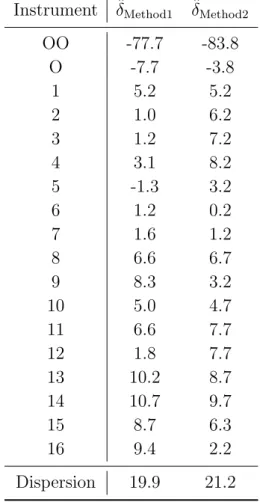
Table 3. Solution of Method 1 and 2 in the realistic synthetic example (Table 2). The values are in microgal and the dispersion is the standard deviation of the offset for both methods. For Method 2 the offsets are shifted by 6.2 µGal with respect to the “true” value.

Instrument δˆMethod1 δˆMethod2

OO -77.7 -83.8 O -7.7 -3.8 1 5.2 5.2 2 1.0 6.2 3 1.2 7.2 4 3.1 8.2 5 -1.3 3.2 6 1.2 0.2 7 1.6 1.2 8 6.6 6.7 9 8.3 3.2 10 5.0 4.7 11 6.6 7.7 12 1.8 7.7 13 10.2 8.7 14 10.7 9.7 15 8.7 6.3 16 9.4 2.2 Dispersion 19.9 21.2

Therefore, instead of imposing ¯ δ = 1 N N X i=1 δi = 0, (13)

we propose to shift the offset values obtained using that assumption by the value ˜δ that

minimizes the L1 norm [10] :

X

i

|˜δ − δi|. (14)

This method is much less sensitive to outliers, as it favors the small individual values rather than the mean value to be small. As explained for instance in [7], it is equivalent to impose a zero median rather than a zero mean. Note that both methods

(zero mean or minimum L1 norm) come down to subtracting a constant value to all the

that will make the L1 norm minimum. Consequently, the error made on the absolute

value is ¯δ in the zero mean case, and ˜δ in the minimum L1 norm case. Our hypothesis,

which we confirm using a numerical experiment here bellow, is that ¯δ > ˜δ in most of

the realistic cases.

To test its behavior with respect to the regular values as well as to outliers, we made the following numerical experiments:

• The offsets of 15 gravimeters were randomly generated using a Gaussian distribution with a unit standard deviation;

• Respectively 5,3,1 and 0 outlying offsets were randomly generated using a Gaussian distribution with a standard deviation equal to 5; this creates sets of respectively 20, 18, 16 and 15 gravimeters. Having a few gravimeters with such outlying offsets is realistic, given the results of the ICAG 2005 [9];

• Knowing the offsets, the actual mean offset was computed and removed from the

offsets of each gravimeter, then the sum of squared errorsP_i(δi− ¯δ)2 was computed;

• The same was done using instead of ¯δ, the value ˜δ that minimizes the L1 norm;

• The process was repeated 100,000 times, which allows us to generate histograms of the error distribution for each case.

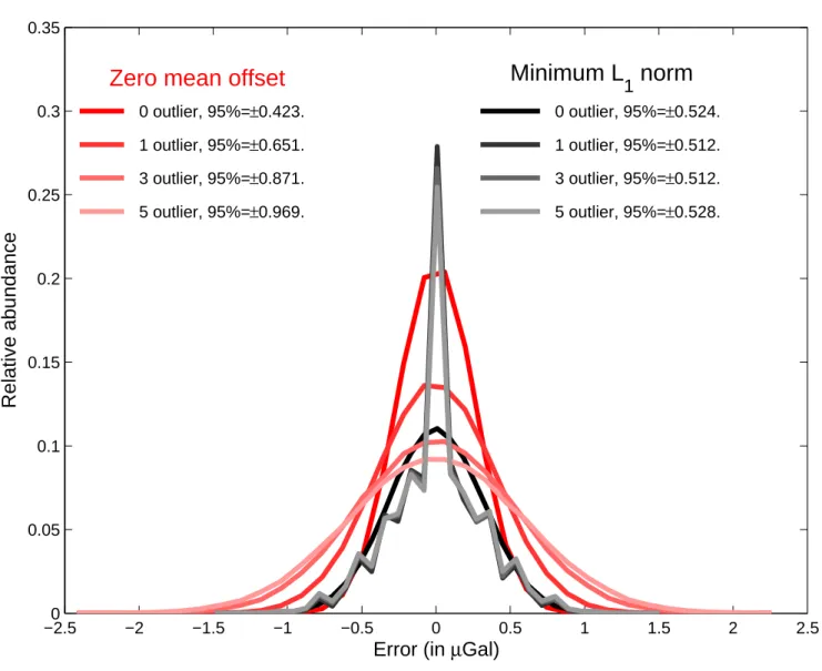
The results are displayed in Figure 1. When applying the L1 norm, 95% of the

results lye in all cases in the [-0.52,0.52] interval, the zero mean method performs slightly better only when there is no outlier, lying in the [-0.43,0.43] interval, but its performances

decrease strongly when the number of outliers increases. As expected from the L1 norm

definition, this simulation confirms that the L1 norm method is barely sensitive to the

outliers, which is not the case for the null average process. Note that the distribution in

case of the L1 norm is not as smooth as the zero mean, because applying the L1 norm

is a non-linear process.

Applying this method on the two synthetic cases presented in Table 1 and Table

2, we obtain, respectively, a shift (i.e. an error) ˜δ = −10 (instead of ¯δ = −16.7) and

˜

δ = −0.5 (instead of ¯δ = −6.1) respectively. Consequently, imposing the minimum L1

norm is better than the zero mean as soon as an outlier is present, and performs slightly worse in cases where no outlier is present (see in Figure 1). The zero mean method is appropriate only if all the gravimeters present similar offsets, equally distributed around

0, but even only one outlier bias the average. The L1 rule favors the gravimeters having

small offsets, providing a better estimate of the absolute offsets, as it is more likely to have a set of instruments with small offsets than having a zero mean value for the whole set of instrument. Note that we also tried with “less outlying” outliers (with a standard

deviation of 3 rather than 5), and the L1 norm solution is still improving the results as

−2.50 −2 −1.5 −1 −0.5 0 0.5 1 1.5 2 2.5 0.05 0.1 0.15 0.2 0.25 0.3 0.35

Zero mean offset

Minimum L

norm

0 outlier, 95%=±0.423. 1 outlier, 95%=±0.651. 3 outlier, 95%=±0.871. 5 outlier, 95%=±0.969. 0 outlier, 95%=±0.524. 1 outlier, 95%=±0.512. 3 outlier, 95%=±0.512. 5 outlier, 95%=±0.528.

Error (in µGal)

Relative abundance

Figure 1. Probability distribution of the error on the offset (in red) and for the minimum L1 norm (black), for different numbers of outlier. Errors are given on the

horizontal axis in unit of the standard deviation, and the number of events on the vertical axis is normalized by the number of experiment.

4.2. Applying the L1 norm method on actual cases

In the real world, the true average value ¯δ is unknown. The Method 2 was applied

in order to determine the instrumental offsets δi. In the least square fit, the normal

equations have been weighted by the uncertainties [11] of the individual measurements. As there is no indication that the measurement errors are normally distributed, we used a bootstrapping method to estimate the instrumental offsets and site gravity values. To this end, we performed 100,000 resampling of the experimental data, keeping constant the number of observations (i.e. allowing replacement, but requesting that each gravimeter appears at least once) as if the sample was the whole population (see for instance [12]). This method allows a fairly robust estimation for large samples, even

if the error distribution is far from being Gaussian. From the 100,000 estimates for the offset of each instrument and of the dispersion of those offsets, we can get a confidence interval for the individual offsets and their dispersion.

The bootstrapping of the data provides mean values for the instrumental offsets δi,

then the minimum L1 criterion is applied and provides ˜δ. This operation does not affect

the higher moments of the distribution of our results, as the same value is subtracted from every single values. The results are presented in the next subsections for the ICAG 2005 and WULG 2007 campaigns.

4.3. The ICAG 2005 experience

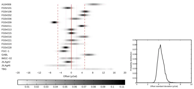
The ICAG 2005 was a comparison of 19 instruments on 12 sites, with 96 measurements provided in Table 2.3.1 in Jiang et al [13]. The equations are weighted by the expanded uncertainties U. The results of the bootstrap evaluation are shown on Figure 2 and in Table 4. Figure 2 (left panel) shows with a gray scale the probability distribution of each offset. The values corresponding to darker area are more probable. Vertical red lines are drawn at values 0 (solid), ±2 (dotted), and ±5 (dashed) µGal. The figure allows a visual comparison of the probability distributions from the different instruments, but the 95% confidence intervals are not shown on the figure, to make it more readible, as they are shown in Figure 3 and given in Table 4.

Figure 2 (right panel) also shows the probability distribution for the offset

dispersion. Note that this distribution, as for the confidence interval of Table 4,

was obtained from the distribution of the offset dispersion obtained from the 100,000 resamplings. The numerical results are summarized in Table 4, where the offset values (in µGal) corresponding to the 5th, the 50th, and the 95th percentile are given for each instrument. The last line shows the 5th, the 50th, and the 95th percentile for the standard deviation of the offsets. These results are compared to the values provided by Vitushkin et al [9] on Figure 3. Note that, unlike the classical least-square error estimation, the bootstrapping method used here allows non centered error bars. This occurs often when an outlying measurement is affecting the data.

4.4. The WULG 2007 experience

For this experience the weights are obtained from the mean set standard deviation plus a systematic error of 2 µGal, as done by Francis et al [6]. The results from the bootstrapping are given in Figure 4 and Table 5. The multi-modal probability distribution of the offset dispersion given on the right panel results from the outlier effect (gravimeter # 20 does not even show up on the left panel). These results are compared to the values provided by Francis et al [6] on Figure 5.

When removing the outlier #20, as done in [6], we got more a reasonable offset dispersion distribution, with the 5th percentile at 2.1, the median at 3.8 and the 95th percentile at 7.2 µGal (Figure 6). If the second outlier #18 is also removed, this becomes 1.8, 2.4 and 4.0 µGal, respectively.

−20 −16 −12 −8 −4 0 4 8 12 16 20 A10#008 FG5#101 FG5#108 FG5#202 FG5#206 FG5#209 FG5#211 FG5#213 FG5#215 FG5#216 FG5#221 FG5#224 FG5#228 FGC−1 GABL IMGC−02 JILAg#2 JILAg#6 TBG Offset (µGal) 0.01 0.02 0.03 0.04 0.05 0.06 0.07 0.08 0.09 0.1 0.11 0 2 4 6 8 10 0 0.01 0.02 0.03 0.04 0.05 0.06 0.07 0.08 0.09

Offset standard deviation (µGal)

Probability distribution

Figure 2. : Result from the bootstrapping of the ICAG 2005 experience. Left panel: Probability distribution for the offset (darker is more likely). Right panel: Probability distribution of the offset dispersion estimated from the whole dataset.

5. Discussion and conclusions

The intercomparison experiments aim at determining the offsets of a set of absolute gravimeters by making them measuring together the same gravity values. The Method 1, used among others in [4], is based on the idea that the subset of gravimeters measuring at the same site has a zero mean offset. The alternative Method 2 was used in [3] and [5], and compared with Method 1 in [6], based on the assumption that the whole set of gravimeters has a zero mean offset.

We have shown both from the mathematical point of view and from the synthetic cases that the Method 1 leads to an underestimation of the absolute value of the offsets, which in turn underestimates the dispersion of the offsets. Consequently, this method should not be used in intercomparison of gravimeters.

The other method is ill-conditioned, and can only be solved if an additional constraint is applied. Since the ICAG 2001 [3], the mean offset is set to zero; this solves the ill-conditioning problem, but imposes a constant on the system: this constant is the actual (unknown) mean offset which is added in the solution to the site gravity values and subtracted to the offset values. Consequently, as the probability of having a null mean offset is weak, we know that the computation gives erroneous results.

The method is not to be blamed for this, as the physical problem is actually ill-conditioned. It is impossible to estimate the offset of a set of instruments simply by comparing them to each other. The Method 2 allows getting a solution, but does not solve the ill-conditioning issue. The hypothesis of zero mean offset is probably better for a larger set of instruments, but it is presently impossible to make it so large that the mean offset would not be an issue.

A10#008 FG5#101 FG5#108 FG5#202 FG5#206 FG5#209 FG5#211 FG5#213 FG5#215 FG5#216 FG5#221 FG5#224 FG5#228 FGC−1 GABL IMGC−02 JILAg#2 JILAg#6 TBG −15 −10 −5 0 5 10 15 20 25 Vitushkin et al., 2010 This study Offset ( µ Gal)

Figure 3. Offsets and error bars as determined by Vitushkin et al [9] (blue) and as given in Table 4.

norm of the offset values. This solution does not provide an exact solution, but it is more robust in case of outliers, as it favors instruments having the smallest offsets. We obtained an offset dispersion of 4.4 µGal (ICAG 2005) and 3.8 µGal (WULG 2007), this value is more robust for the 2005 campaign than for the 2007, where the bootstrapping has shown a strong variability under resampling, which is due to strongly biased gravimeters. This problem can be solved by excluding the biased gravimeters from the calculations.

From the results shown here, we also confirm that a single instrument is not likely to provide alone measurements at the microgal level accuracy. On the other hand, when comparing two measurements performed with the same instrument, the time change of the gravity can be determined with such an accuracy, given that no instrumental drift (for instance on the laser) occurred and that the instrumental setup is exactly the same

−20 −16 −12 −8 −4 0 4 8 12 16 20 1 2 3 4 5 6 7 8 9 10 11 12 13 14 15 16 17 18 19 20 Offset (µGal) 0 0.01 0.02 0.03 0.04 0.05 0.06 108 110 112 114 116 118 120 122 124 0 0.005 0.01 0.015 0.02 0.025 0.03 0.035

Offset standard deviation (µGal)

Probability distribution

Figure 4. Result from the bootstrapping of the WULG 2007 regional comparison. Left panel (A): Probability distribution for the offset values (darker is more likely; for the instrument #20 the offset lies outside the graph limits). Right panel (B): Probability distribution of the offset dispersion estimated from the whole dataset. This value is strongly influenced by the gravimeter # 20.

FG5#101 FG5#222 FG5#202 FG5#206 FG5#211 FG5#215 FG5#216 FG5#218 FG5#220 FG5#221 FG5#226 FG5#228 FG5#229 FG5#230 FG5#232 FG5#233 FG5#234 IMGC#2 Jilag−6 −15 −10 −5 0 5 10

Francis et al., 2010 (#20 excl.)

This study

This study (#20 excl.)

Offset (

µ

Gal)

Figure 5. Offsets and error bars as determined by Francis et al [6] (blue), as given in Table 5 (red) and obtained by method 2 when the # 20 has been removed (green).

Table 4. ICAG 2005: 5th, 50th, and 95th percentile estimations for the offset of each instrument (in µGal). The last line shows the estimation of dispersion equivalent to the standard deviation of the offsets for the whole set of instruments. Note that this value is obtained directly from the bootstrapping, and is thus not equal to the standard deviation of the above numbers.

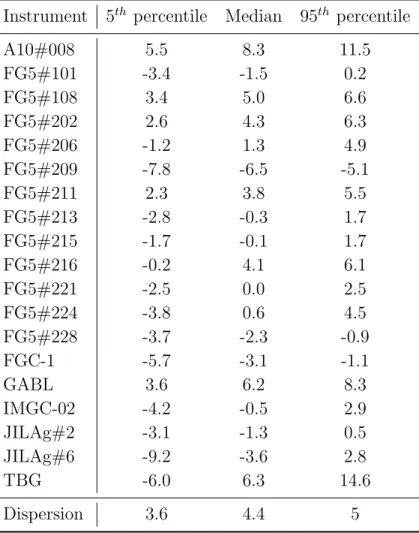
Instrument 5th _{percentile Median 95}th _percentile

A10#008 5.5 8.3 11.5 FG5#101 -3.4 -1.5 0.2 FG5#108 3.4 5.0 6.6 FG5#202 2.6 4.3 6.3 FG5#206 -1.2 1.3 4.9 FG5#209 -7.8 -6.5 -5.1 FG5#211 2.3 3.8 5.5 FG5#213 -2.8 -0.3 1.7 FG5#215 -1.7 -0.1 1.7 FG5#216 -0.2 4.1 6.1 FG5#221 -2.5 0.0 2.5 FG5#224 -3.8 0.6 4.5 FG5#228 -3.7 -2.3 -0.9 FGC-1 -5.7 -3.1 -1.1 GABL 3.6 6.2 8.3 IMGC-02 -4.2 -0.5 2.9 JILAg#2 -3.1 -1.3 0.5 JILAg#6 -9.2 -3.6 2.8 TBG -6.0 6.3 14.6 Dispersion 3.6 4.4 5

for the two measurements. 6. Acknowledgments

The contribution of OdV to this study is IPGP contribution XXXX. This study benefited from a grant of the Space Campus of the University Paris Diderot. Discussions with G. Pajot-M´etivier were helpful to this paper. The two referees are acknowledged for their carreful review, which helped improving this paper.

7. Bibliography

[1] Faller J., 2002, Thirty years of progress in absolute gravimetry: a scientific capability implemented by technological advances, Metrologia, 39, 425-428.

Table 5. WULG 2007: 5th, 50th, and 95th percentile estimations for the offset of each instrument (in µGal). The last line shows the estimation of the dispersion equivalent to the standard deviation of the offsets for the whole set of instruments. Note that this value is obtained directly from the bootstrapping, and is thus not equal to the standard deviation of the above numbers.

Instrument 5th _{percentile Median 95}th _percentile

1 FG5#101 -0.1 2.1 4.6 2 FG5#222 -1.6 0.6 3.2 3 FG5#202 -0.2 3.3 6.5 4 FG5#206 -4.6 -1.5 1.7 5 FG5#211 -0.3 2.6 5.9 6 FG5#215 -1.8 0.5 2.8 7 FG5#216 -0.6 1.5 3.6 8 FG5#218 -8.0 -4.1 -0.9 9 FG5#220 -0.8 2.2 5.2 10 FG5#221 -3.0 0.0 2.6 11 FG5#226 -8.5 -3.6 0.5 12 FG5#228 -2.8 -0.5 2.1 13 FG5#229 -4.1 -1.5 1.1 14 FG5#230 -3.0 -0.2 2.8 15 FG5#232 -1.3 1.4 4.0 16 FG5#233 -1.7 0.5 3.0 17 FG5#234 -3.2 -0.8 2.0 18 IMGC#2 -24.3 -12.4 -2.8 19 Jilag-6 -3.7 0.5 4.4 20 MPG#2 490 514.5 532.0 Dispersion 109.4 115.5 119.8

[2] Eichenberger A., Jeckelmann B., and Richard P., 2003, Tracing Planck’s constant to the kilogram by electromechanical methods Metrologia, 40, 356-365.

[3] Vitushkin L., Becker M., Jiang Z., Francis O., van Dam T.M., Faller J., Chartier J.-M., Amalvict M., Bonvalot S., Debeglia S., Desogus S., Diament M., Dupont F., Falk R., Gabalda G., Gagnon C.G.L., Gattacceca T., Germak A., Hinderer J., Jamet O., Jeffries G., Kter R., Kopaev A., Liard J., Lindau A., Longuevergne L., Luck B., Maderal N., Mkinen J., Meurers B., Mizushima S., Mrlina J., Newell D., Origlia C., Pujol E.R., Reinhold A., Richard P., Robinson I., Ruess D., Thies S., Van Camp M., Van Ruymbeke M., de Villalta Compagni M.F., and Williams S., 2002, Results of the Sixth International Comparison of Absolute Gravimeters, ICAG-2001, Metrologia, 39, 407-424.

[4] Robertsson L., Francis O., van Dam T.M., Faller J., Ruess D., Delinte J.-M., Vitushkin L., Liard J., Gagnon C., Guo You Guang, Huang Da Lun, Fang Yong Yuan, Xu Jin Yi, Jeffries G., Hopewell H., Edge R., Robinson I., Kibble B., Makinen J., Hinderer J., Amalvict M., Luck B.,Wilmes H., Rehren F., Schmidt K., Schnull M., Cerutti G., Germak A., Zabek Z., Pachuta A., Arnautov

1 2 3 4 5 6 7 8 9 0 0.02 0.04 0.06 0.08 0.1 0.12 0.14 0.16 0.18 0.2

Offset standard deviation (µGal)

Probability distribution

# 18,20 removed # 20 removed

Figure 6. Probability distribution of the offset dispersion from the bootstrapping of the WULG 2007 comparison, with the gravimeters #20 (red) and #18, 20 (black) not taken into account.

G., Kalish E., Stus Y., Stizza D., Friederich J., Chartier J.-M., and Marson I., 2001, Results from the fifth international comparison of absolute gravimeters, ICAG’97 Metrologia, 38, 71-78. [5] Francis O., van Dam T., Amalvict M., Andrade de Sousa M., Bilker M., Billson R., D’Agostino G., Desogus S., Falk R., Germak A., Gitlein O., Jonhson D., Klopping F., Kostelecky J., Luck B., Mkinen J., McLaughlin D., Nunez E., Origlia C., Palinkas V., Richard P., Rodriguez E., Ruess D., Schmerge D., Thies S., Timmen L., Van Camp M., van Westrum D., and Wilmes H., 2005, Results of the International Comparison of Absolute Gravimeters in Walferdange (Luxembourg) of November 2003 In International Association of Geodesy Symposia Gravity, Geoid and Space Missions GGSM 2004, Vol. 129 (XVI) ed C Jekeli, L Bastos and J Fernandes (Springer-Verlag), pp 272-275

[6] Francis O., van Dam T.M., Germak A., Amalvict M., Bayer R., Bilker-Koivula M., Calvo M., D’Agostino G.C., Dell’Acqua T., Engfeldt A., Faccia R., Falk R., Gitlein O., Fernandez M., Gjevestad J., Hinderer J., Jones D., Kostelecky J., Le Moigne N., Luck B., Mkinen J., Mclaughlin D., Olszak T., Olsson P., Pachuta A., Palinkas V., Pettersen B., Pujol E.R., Prutkin I., Quagliotti D., Reudink R., Rothleitner C., Ruess D., Shen C., Smith V., Svitlov S., Timmen L., Ulrich C., Van Camp M., Walo J., Wang L., Wilmes H., and Xing L., 2010, Results of the European Comparison of Absolute Gravimeters in Walferdange (Luxembourg) of November 2007 Gravity, Geoid and Earth observation, International Association of Geodesy Symposia, Vol. 135 (XII) ed SP Mertikas (Berlin Heidelberg: Springer-Verlag) pp 31-36, DOI 10.1007/978-3-642-10634-7 5 [7] Dodge, Y, 1987, An introduction to L1-norm based on statistical data analysis. Comptational

Statistics and Data Analysis, 5, 329-253.

[8] Cox M.G., 2002, The evaluation of key comparison data, Metrologia, 39,589-595.

[9] Vitushkin L., Jiang Z., Robertsson L., Becker M., Francis O., Germak A., D’Agostino G., Palinkas V., Amalvict M., Bayer R., Bilker-Koivula M., Desogus S., Faller J., Falk R., Hinderer J.,

Gagnon C., Jacob T., Kalish E., Kostelecky J., Lee C., Liard J., Lokshyn Y., Luck B., Mkinen J., Mizushima S., Le Moigne N., Nalivaev V., Origlia C., Pujol E.R., Richard P., Ruess D., Schmerge D., Stus Y., Svitlov S., Thies S., Ullrich C., Van Camp M., Vitushkin A., and Wilmes H., 2010, Results of the Seventh International Comparison of Absolute Gravimeters ICAG-2005 at the Bureau International des Poids et Mesures, Svres Gravity, Geoid and Earth observation, International Association of Geodesy Symposia, Vol. 135 (XII) ed SP Mertikas (Berlin Heidelberg: Springer-Verlag) pp 47-54, DOI: 10.1007/978-3-642-10634-7 7

[10] Barton R.R. and Ivey J.S., 1996, Nelder-Mead simplex modifications for simulation optimization Management, Science, 42, 954-973

[11] Kay S. M., 1993, Fundamentals of Statistical Signal Processing: Estimation Theory (Upper Saddle River New Jersey: Prentice Hall) 625 p.

[12] Moore D.S., McCabe G.P., Duckworth W.M., and Sclove S.L., 2003, The practice of business statistics: Using data for decisions, 2nd ed. (New York: WH Freeman) 859 p

[13] Jiang Z., Francis O., Vitushkin L., Palinkas V., Germak A., Becker M., D’Agostino G., Amalvict M., Bayer R., Bilker-Koivula M., Desogus S., Faller J., Falk R., Hinderer J., Gagnon C., Jacob T., Kalish E., Kostelecky J., Lee C., Liard J., Lokshyn Y., Luck B., Mkinen J., Mizushima S., Le Moigne N., Origlia C., Pujol E.R., Richard P., Robertsson L., Ruess D., Schmerge D., Stus Y., Svitlov S., Thies S., Ullrich C., Van Camp M., Vitushkin A., Wang J., and Wilmes H., 2011, Review of the Seventh International Comparison of Absolute Gravimeters (ICAG 2005) - a pilot study toward the CIPM Key Comparison, Metrologia, (submitted)