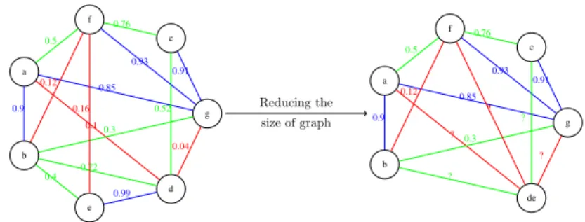
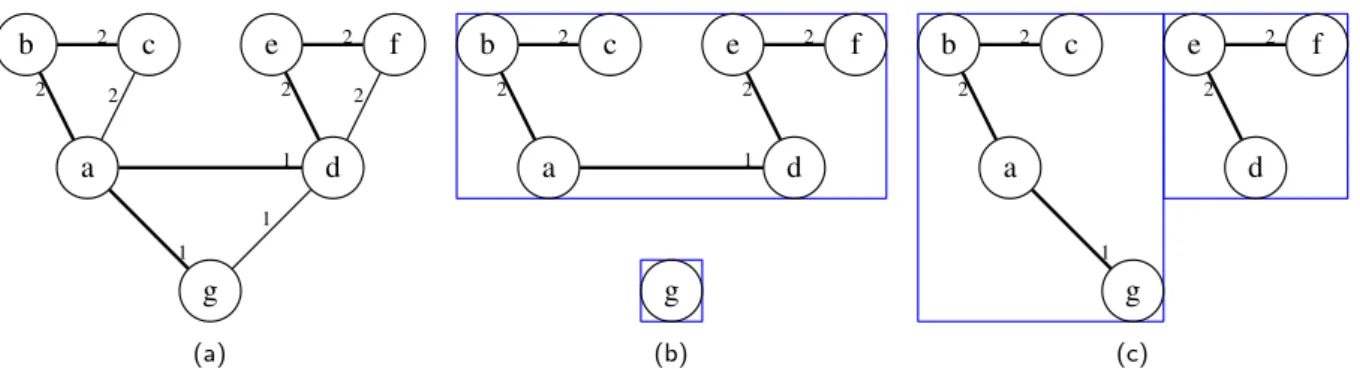
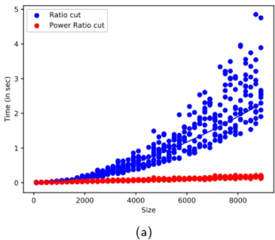
Power Spectral Clustering

HAL Id: hal-01516649

https://hal.archives-ouvertes.fr/hal-01516649v4

Submitted on 25 Jun 2020

HAL is a multi-disciplinary open access

archive for the deposit and dissemination of

sci-entific research documents, whether they are

pub-lished or not. The documents may come from

teaching and research institutions in France or

abroad, or from public or private research centers.

L’archive ouverte pluridisciplinaire HAL, est

destinée au dépôt et à la diffusion de documents

scientifiques de niveau recherche, publiés ou non,

émanant des établissements d’enseignement et de

recherche français ou étrangers, des laboratoires

publics ou privés.

Power Spectral Clustering

Aditya Challa, Sravan Danda, B S Daya Sagar, Laurent Najman

To cite this version:

Aditya Challa, Sravan Danda, B S Daya Sagar, Laurent Najman. Power Spectral Clustering. Journal

of Mathematical Imaging and Vision, Springer Verlag, 2020, 62 (9), pp.1195–1213.

�10.1007/s10851-020-00980-7�. �hal-01516649v4�

(will be inserted by the editor)

Power Spectral Clustering

Aditya Challa · Sravan Danda · B. S. Daya Sagar · Laurent Najman

Received: date / Accepted: date

Abstract Spectral clustering is one of the most impor-tant image processing tools, especially for image segmen-tation. This specializes at taking local information such as edge weights and globalizing them. Due to its unsuper-vised nature, it is widely applicable. However, traditional

spectral clustering is O(n3/2_{). This poses a challenge,}

especially given the recent trend of large datasets. In this article, we propose an algorithm by using ideas from Γ −convergence, which is an amalgamation of Maximum Spanning Tree (MST) clustering and spectral cluster-ing. This algorithm scales as O(nlog(n)) under certain conditions, while producing solutions which are similar to that of spectral clustering. Several toy examples are used to illustrate the similarities and differences. To val-idate the proposed algorithm, a recent state-of-the-art technique for segmentation - multiscale combinatorial grouping is used, where the normalized cut is replaced with the proposed algorithm and results are analyzed. Keywords Spectral clustering, Γ −convergence, MST-based clustering, Multiscale combinatorial grouping, Image segmentation.

Aditya Challa,

Systems Science and Informatics Unit, Indian Statistical In-stitute, 8th Mile Mysore Road, Bangalore, India.

E-mail: aditya.challa.20@gmail.com Sravan Danda

Systems Science and Informatics Unit, Indian Statistical In-stitute, 8th Mile Mysore Road, Bangalore, India.

E-mail: sravan8809@gmail.com B. S. Daya Sagar

Systems Science and Informatics Unit, Indian Statistical In-stitute, 8th Mile Mysore Road, Bangalore, India.

E-mail: bsdsagar@yahoo.co.uk,bsdsagar@isibang.ac.in Laurent Najman

Université Paris-Est, LIGM, Equipe A3SI, ESIEE, France. E-mail: laurent.najman@esiee.fr

1 Introduction

Spectral clustering has been widely popular due to its usage in image segmentation [32]. It plays an impor-tant role in globalizing local information in the recent state-of-the-art method for segmentation - multiscale combinatorial grouping [30]. Although convolution neu-ral networks form the current state-of-the-art for image segmentation [26], this can be attributed to the avail-ability of huge labelled datasets. There exists domains where data is not easy to obtain, such as hyperspec-tral image datasets, where unsupervised techniques can be very useful. In methods such as those described in [35], even after using convolution neural nets, spectral clustering is used as the last step for segmentation.

An overview of spectral clustering procedures can be found in [38]. One of the reasons for the popular-ity of the spectral clustering procedure is its abilpopular-ity to detect non-convex clusters. Spectral clustering method proceeds by constructing an edge-weighted graph from the data and use the eigenvectors of the Laplacian of the graph. However, the calculation of the eigenvectors is computationally expensive, and is prone to errors. Several efforts were made to increase the speed and ac-curacy of the spectral clustering methods [42, 10, 17, 18], including parallelizing [34]. In [30], the authors propose to reduce the size of the similarity matrix to speed up the normalized cuts procedure for image segmentation [32].

Another clustering method which allows to detect non-convex clusters is that of Maximum Spanning Tree (MST) based clustering [43]. This method proceeds by constructing an MST on the edge-weighted graph and by removing the edges with least similarity. The main advantage of this method is that it is fast and scales well for big data. However, these methods also have some

a b 0.9 d 0.1 f 0.5 g 0.85 0.72 e 0.4 0.3 c 0.52 0.76 0.91 0.99 0.04 0.16 0.12 0.93 a b 0.9 de ? f 0.5 g 0.85 ? 0.3 ? ? 0.12 0.93 c ? 0.76 0.91 Reducing the size of graph

Fig. 1 Figure illustrating the motivation of the article. On the left we have an example graph with the edge weights denoting the similarities. The objective is to perform clustering such as spectral clustering. Intuitively, it is easy to infer that nodes d and e would belong to the same cluster as they have the similarity of 0.99. Hence, there is a scope to reduce the computations required. However, it is not obvious to decide on which similarity values should be considered high enough so as to merge the corresponding incident nodes. Moreover, assume we have indeed reduced the graph size by merging nodes, as in figure on the right. It is not clear what the edge weights in the contracted graph would be? These questions are answered using the power watershed framework.

ambiguity in clusters and results in degenerate solutions. (MST-based clustering is discussed in detail in section

2.)

In this article, the aim is to develop an algorithm which uses efficient MST-based clustering within a ter and more computationally expensive spectral clus-tering near the borders of the clusters. This is achieved by computing the limit of minimizers (a.k.a Γ −limit) of spectral clustering. We obtain a faster version of spectral clustering while preserving the properties of spectral clustering, referred to as power spectral clus-tering or Power Ratio cut or more simply PRcut. The study of Γ −limits is referred to as the Γ −convergence. Γ −convergence is widely used in the areas of computer vision and in the field of calculus of variations (See chapter 5 of [6]). In [11], the authors proposed Power Watershed - Γ −limit of the energy function in [33] and demonstrated its similarity with watershed transforma-tion [12, 13]. It turns out that the Power Watershed performs better in several cases compared to the fre-quently used seeded segmentations. In [27], the power watershed framework was extended and a simple generic algorithm was proposed to calculate the limit of min-imizers under some conditions. Other applications of the power watershed framework can be found in [16, 15, 40]. The methods described in [16, 15, 40] use power watershed framework to reduce the size of the graph. In this article, we propose to use power watershed frame-work for spectral clustering - by computing a Γ −limit of spectral clustering. This article is a significant extension of the conference version [8]. The following are main contributions of this article

-1. A novel algorithm for clustering, PRcut, is proposed. Using power watershed framework, it is shown that PRcut is faster than spectral clustering while giving

similar results. Also, efficient algorithm for imple-menting PRcut is proposed.

2. Several properties of PRcut are exhibited by using toy examples and compared with MST-based clus-tering and spectral clusclus-tering.

3. To conclusively show that PRcut can be used in place of spectral clustering, application to multiscale combinatorial grouping (MCG)[30] is demonstrated. Specifically, the spectral clustering step in MCG is replaced with the proposed method and empirically shown that PRcut is faster while preserving the overall accuracy of the method.

4. The concept of discretization of the weights is intro-duced. This adds further flexibility to the PRcut, in the sense that in the base case PRcut is equivalent to spectral clustering. Thus, PRcut can be considered an extension of spectral clustering as well.

5. Applications to hyperspectral images and high di-mensional datasets are also discussed.

The outline of the article is as follows - In section 2, various concepts required for the rest of the article -spectral clustering, MST clustering and Γ −convergence, are introduced. In section 3, we start with a generic algorithm to calculate a Γ −limit and characterize differ-ent parts of the algorithm to obtain an implemdiffer-entable version. In section 4, we further increase the efficiency by identifying the relation between eigenvectors and connected components of the Laplacian. In section 5, we explore the PRcut in detail. We compare PRcut with MST-based clustering and spectral clustering using several toy examples to illustrate the differences and similarities. To validate the claim that PRcut is similar to classic spectral clustering, we use multiscale combina-torial grouping (MCG). MCG [30] was a state-of-the-art algorithm for segmentation which used spectral cluster-ing as a step in the pipeline. We replace this step with

the PRcut algorithm and compare the results. It can be deduced that the PRcut algorithm is faster than spectral clustering while giving similar results. Also shown are applications to hyperspectral image data.

Gist of the article: As stated earlier, in this article we develop an algorithm which combines the efficiency of MST-based clustering within a cluster and accuracy of spectral clustering at the boundaries. This is achieved by considering the Γ −limit of the spectral clustering, To compute the said Γ −limit we use the power watershed framework developed in [27]. The solution thus obtained is referred to as power spectral clustering or PRcut.

To understand the redundancies Power Spectral Clus-tering exploits, consider a simple graph as shown in fig-ure 1. The edge weights shown indicate the similarities between the end points of the edge. Intuitively, it is clear that computations are not required to infer that the nodes d and e would belong to the same cluster since

they have a similarity of0.99. Similarly, e and f does

not belong to the same cluster since their similarity is 0.1.

However, it is not clear as to where to make a clear distinction? That is, picking a threshold. Moreover,

as-sume we have contracted the edge(d, e) considering a

single node for d and e, as shown in figure 1. It is not clear what the new edge weights would be? These ques-tions are implicitly answered when one considers the limit of minimizers, which is obtained using the power watershed framework. As it would be illustrated in this article, the power watershed limit results in algorithm 4.

2 Background

The main mathematical structure used in this article is

that of an edge-weighted graph - G= (V, E, W ). Given

an image I, the set of vertices is taken as the pixels in I, the set of edges is given by the 4-adjacency relation.

The edge weights W : E → R+_{are constructed by using}

the pixel values. The edge weights are assumed to reflect the similarity between two pixels/points.

Note that both spectral clustering and MST clus-tering operate on edge-weighted graphs. Thus, these methods can be used on any data which can be rep-resented as edge-weighted graphs. For data in general euclidean space, k-nearest neighbors graph is used [38]. In this article, small toy examples of general data are also used for better analysis.

D is a diagonal matrix, diag(d1, d2, · · · , dn), such

that

di=

X

j

wij (1)

The Laplacian of a graph is defined by

L= D − W (2)

We know that the Laplacian is a symmetric positive-semi-definite matrix, and hence has non-negative real

eigenvalues. The eigenvalues are represented by 0 =

λ1≤ λ2≤ · · · ≤ λn. The corresponding eigenvectors are

denoted by {e1, e2, · · · , en}. Let A ⊆ V . Denote

1A(x) =

(

1 if x ∈ A 0 otherwise

G≥w denotes the thresholded graph, with vertex set

V and edge set, E≥w, consisting of only those edges

whose weights are greater than or equal to w.

2.1 Spectral Clustering

Spectral clustering methods work by projecting the data onto a subspace, so that similar points are close by and dissimilar points are far apart in the projected subspace. There are 3 steps which form the core of spectral clustering

methods-1. Given a set of points {xi} (dataset), construct a

graph, G, with each data point as a vertex.

2. Construct the Laplacian for the obtained graph and calculate the first m eigenvectors of the Laplacian. The value of m is fixed based on the number of clusters required. Let H be the matrix such that the

ith _{column of H is the i}th _{eigenvector e}

i.

3. Using rows of the matrix H as new representation of

the points xi, use classical clustering methods such

as k-means to obtain the final clusters.

The Laplacian in (2) is known as an unnormalized Laplacian. Some works also consider the normalized

Laplacians, L1, L2as well [32, 29], where,

L1= I − D−1W; L2= I − D−1/2W D−1/2 (3)

Why does spectral clustering work? The idea behind working of spectral clustering methods can be intuitively understood using two results - (i) Suppose the

graph G has m connected components, {A1, A2, · · · , Am}.

Then the basis of the vector space spanned by the first m

eigenvectors is {1A1, 1A2, · · · , 1Am} and (ii) The

eigen-spaces of a matrix and its perturbation are ‘close’ [38]. Assume that the similarity between points from two different clusters is small, and similarity between points from same cluster is high. Then, from the above results, the first few eigenvectors of the Laplacian are close to the indicator of the clusters. Hence simple clustering methods work well on this projected data.

2.1.1 Different formulations of spectral clustering The spectral clustering can also be analyzed in an

op-timization framework. Given a similarity graph G =

(V, E, W ), consider the graph cut measure

cut(A1, A2, · · · , Am) = 1 2 m X i=1 W(Ai, Ai) (4) where W(A, B) = X i∈A;j∈B wij (5)

A denotes the complement of A in the vertex set V . m denotes the size of the partition required which is equal to the number of clusters. Note that cut(., .) measures how similar the clusters are by taking the sum of the weights of the edges connecting distinct clusters, and hence can be used to partition a graph. In practice, however, minimizing the cut(., .) does not give good results, since it generally separates one vertex, and gives degenerate solutions. Also, minimizing cut(., .) for m ≥ 3 is NP-hard [36]. Thus, it was proposed to use a variation of the above cost function. Ratio cut [38] is given by

Rcut(A1, A2, · · · , Am) = 1 2 m X i=1 W(Ai, Ai) |Ai| (6)

Here |Ai| is the cardinality of set Ai. Note that ratio cut

penalizes small clusters, and hence avoids degenerate solutions. Let G be a graph constructed from the data set, and let L denote its corresponding Laplacian. It is shown that minimizing the Rcut(., .) for m clusters is approximately equivalent to solving the optimization problem in (7) [38]. minimize H∈Rn×m T r(H t_LH) subject to HtH = I (7)

where, I is the identity matrix. From the Rayleigh-Ritz theorem, it is known that the solution to optimization problem in (7) is obtained by considering the first m eigenvectors of L as columns of H [25].

Another variation of the cut(., .) cost function, pro-posed in [32] is the Normalized cut (Ncut) cost function given by N cut(A1, A2, · · · , Am) = 1 2 m X i=1 W(Ai, Ai) vol(Ai) (8)

where vol(Ai) = P_idi. It can be shown that for m

clusters, N cut(., .) is approximately equivalent to the solution of the following optimization problem[38]. minimize H T r(H t_LH ) subject to HtDH = I (9)

It is known that the solution to this optimization prob-lem is obtained by taking the first m eigenvectors of

I − D−1W as columns of H [25].

2.2 Maximum Spanning Tree Clustering

Another method of clustering which can detect non glob-ular clusters in the data is maximum spanning tree based

clustering. Let G= (V, E, W ) be a connected similarity

graph. A spanning tree, T , is a connected acyclic sub-graph of G whose vertex set is V . Each spanning tree can be assigned a numerical value by taking the sum of the weights of the edges in the tree,

w(T ) = X

e∈E(T )

w(e) (10)

A spanning tree with the maximum weight is known as the Maximum Spanning Tree (MST). There are sev-eral clustering methods based on MST [43]. Although MST-based clustering is not so prevalent in cluster-ing general data, in the context of image segmentation, slight variations of MST-based clustering was shown to be very useful, thanks to its equivalence to water-sheds (as described in [12, 13]). A generic MST-based clustering algorithm is

1. Given a similarity graph G = (V, E, W ), construct

an MST, T , and sort the edges of T according to the weights.

2. If the required number of clusters is equal to m, add edges starting from highest weight until the number of components m are reached. The ties are broken arbitrarily.

MST-based clustering is categorized under graph based clustering, and is related to the hierarchical approaches. In fact, MST-based clustering as described above is equivalent to single link hierarchical clustering.

The main problems with MSTbased clustering are -(i) It is prone to noise and outliers, (ii) In practice, it gives small clusters or degenerate solutions which are not so meaningful, and (iii) Arbitrariness in breaking of ties results in non uniform solutions. In the later sections it will be seen that the proposed method, PRcut, is similar to MST-based clustering and does not suffer from these problems.

2.3 Γ -convergence and Power Watershed Framework

Let min{Fi(x) : x ∈ X} be a sequence of minimum

problems. A question of interest is the limiting behav-ior of the minimizers of this family as i → ∞. Ideally this would be substituted by a single minimum problem

min{F (x) : x ∈ X} which captures the limiting behavior. Few of the advantages of such a substitution are -1) This gives an approximate solution to the family of minimizers which are much harder to calculate than the limit, 2) Dependence on a parameter is nullified, and 3) This results in a new method which would present a

different model which was previously modeled with Fi.

The theory of Γ −convergence focusses on understand-ing the conditions under which such a substitution is possible [6].

In this article, however, we are interested in calculat-ing a Γ −limit of the spectral clustercalculat-ing discussed above. Recently the authors in [11] calculated Γ −limit of the seeded random walker cost function [33], and proposed Power watershed seeded segmentation. This Γ −limit involves an MST, and hence links the random walk segmentation with MST clustering. In [27], a generic algorithm was proposed to calculate a Γ −limit, which we review here.

Let 0 < α1 < α2 < · · · < αk ≤ 1 and Qi(x) is

continuous for all i. Consider the cost function

Q(p)(x) =

k X

i=0

αp_iQi(x) (11)

The problem is to calculate the limit of minimizers of

Q(p)_{(x) as p → ∞. Observe that the function itself}

converges to 0 at every point if αk < 1, and hence

minimizers of the limit would be the whole space. Let C be a compact set. For the sake of simplicity, we assume that we are interested in finding the solutions in C. Define

Mk= arg min

x∈C

Qk(x) (12)

i.e, Mk is the set of minimizers for Qk. Now recursively

define, for i= k − 1, · · · , 1.

Mi= arg min

x∈Mi+1

Qi(x) (13)

Observe that we have the following relation between Mi,

i= 1, · · · , k.

Mi⊆ Mj for all1 ≤ i < j ≤ k (14)

Theorem 1 ([27]) Let X∗ be the union of the sets of

minimizers of Q(p) _{(as defined in (11)) for all p. Then}

every limit point of X∗ belongs to the set M1.

The above theorem can be interpreted in terms of scale.

If one interprets each αi as a scale, then theorem 1

states - Γ −limit (limit of minimizers) belongs to the set of solutions which minimizes all the cost functions

at different scales αi starting from the largest scale αk.

The main consequence of theorem 1 is that one can now formulate algorithm 1 to calculate a Γ −limit [27].

Algorithm 1 Generic Algorithm to Compute Γ −limit.

Input: Function Q(p)_{(x) =}Pk i=1α p iQi(x), where 0 ≤ α1< α2< · · · < αk≤ 1. Output: M1

1: Mk= arg min Qk(x) where x ∈ C

2: for i from k − 1 to 1 do

3: Compute Mi= arg min Qi(x) where x ∈ Mi+1

4: end for

Theorem 1 ensures that a Γ −limit belongs to the output of algorithm 1. The converse is not true in gen-eral, i.e, all solutions obtained from algorithm 1 need not be a Γ −limit. However, it can be shown that they are ‘equivalent’, in the sense that the value of the cost function is same for all p, and hence in the limit as well.

Proposition 1 Let x∗ be a Γ −limit for Q(p). Letx be_b

a solution obtained from algorithm 1. Then we have that, for all p

Q(p)(x∗) = Q(p)₍

b

x) (15)

The proof of the proposition 1 is straightforward. Although algorithm 1 might not calculate a Γ −limit, we have that it calculates equivalent solution as far as the cost function is concerned.

In the special case when Q(x) is taken to be the ratio cut cost function, we have the converse as well. This is described in theorem 2.

To summarize, we have computed the Γ −limit for the cost functions of the form in (11). This resulted in a generic algorithm 1. This is referred to as Power Watershed framework in the rest of this article. The limit obtained by using the algorithm 1 is also referred to as Power Watershed limit. Detailed analysis of the Power Watershed and its relation to existing works can be found in [27].

3 Γ −limit of spectral clustering

In several cases discrete models are used for modeling the data, while the data might be continuous. This is especially true in the case of graph-based models [11]. Thus a discretization scheme is required for using dis-crete models in real data. We introduce the definition of a discretization scheme which is then used for calculating a Γ −limit.

Let G= (V, E, W ) be a graph. Recall that W : E →

Definition 1 (Discretization Scheme) A discretiza-tion scheme is a decomposidiscretiza-tion of W , i.e for all edges e, we have

W(e) = cW(e)ω(e) (16)

where cW : E → Z+ _{and ω}

: E → R+_{, with a condition}

that if W(e1) < W (e2), then cW(e1) < cW(e2).

An example of a discretization scheme is given by taking the least integer function.

W(e) = bW (e)c W(e)

bW (e)c = cW(e)ω(e) (17)

Here cW(e) = bW (e)c and ω(e) = W (e)/bW (e)c.

Intu-itively, cW is the discrete version of W and ω is error

with respect to the discretization. It is also clear that there are several discretization schemes possible.

As another example, one can consider the following decomposition of the weights

W(e) = bcW (e)c W(e)

bcW (e)c = cW(e)ω(e) (18)

where c is an arbitrary positive constant. An exponentiated graph is denoted by

G(p)= (V, E, W(p)) (19)

where W(p)_{(e) = (cW(e))}p_{ω(e). Accordingly we can}

de-fine D(p), a diagonal matrix,

[D(p)_] ii= X j W_ij(p) (20) and a Laplacian L(p) _{= D}(p)_{− W}(p)_.

We define a Γ −limit of spectral clustering by the limit of minimizers of the optimization problem (21) as p → ∞. minimize H∈Rn×m T r(H t_L(p)_H) subject to HtH = I (21)

In the case of the optimization problem theorem (21) as above, teh converse of 1 holds. This is summarized in the following theorem.

Theorem 2 Given the notation as in theorem 1, and

considering the Q(p) _{to be the optimization problem in}

(21), we have that any point in M1 is a limit point of

X∗_.

The proof of the above theorem is given in the ap-pendix.

Since the datasets are finite, cW takes only finite

number of values. Also, since the optimization problem does not change with positive scalar multiples, one can

assume without loss of generality that the distinct values

may be denoted by 0 < w1 < w2 < · · · < wk < 1,

indicating the k distinct weights cW(e) can take. Denote

by Githe graph with the vertex set, V , and the edge set

consisting of only those edges e such that cW(e) = wi.

The weight of an edge e in Gi is given by the function

ω(e). The Laplacian for the graph Gi is denoted by Li.

Then it is easy to see that

L= k X i=1 wiLi (22) and hence, T r(Ht_{LH) =} k X i=1 wiT r(HtLiH) (23)

Accordingly, for the exponentiated graphs we have

T r(HtL(p)H) =

k X

i=1

wp_iT r(HtLiH) (24)

Note that (24) is in the form of (11) and hence we can use the generic algorithm 1 to calculate a Γ −limit.

Let M denote the set of all possible m dimensional

subspaces of Rn_{. Each subspace in M can be associated}

with an n × m matrix H, such that the column space of H is the subspace. Note that this matrix is not unique. Also, let H(M ) denote the set of all matrices whose column space is equivalent to any of the subspaces in

the set M . Let M(H) denote the set of all column spaces

of matrices in a set of matrices H. It is easy to see that the following relations hold true.

M(H(M0_{)) = M}0

H(M(H0_{)) ⊇ H}0

where M0 is a set of subspaces and H0 is a set of

matrices. With this notation, the generic algorithm 1 in the case of ratio cut optimization would be the one in algorithm 2. However, this algorithm is not imple-mentable. One needs to characterize all the solutions to the optimization problem in (7) to obtain an

imple-mentable version. This will in turn characterize the Mi

Algorithm 2 Generic Algorithm to Compute Γ −limit.

Input: A weighted graph, G, with distinct weights w1 <

w2< · · · < wk. Number of clusters to calculate m.

Output: M0

1: Set i = k, Mi= M

2: Construct the graph Giat level i, and Laplacian Li.

3: Solve the optimization problem minimize H∈Rn×m T r(H t_L iH) subject to Ht_{H = I} H ∈ H(Mi) (25)

4: Let Hi be the set of possible minimizers of the above

optimization problem. Set Mi−1= M(Hi).

5: Set i = i - 1 6: if i = 0 then 7: Stop. 8: return M0 9: else 10: Goto Step (2) 11: end if

3.1 Solutions to ratio cut optimization problem

Given a Laplacian L of dimensions n × n, let λ1≤ λ2≤

· · · ≤ λn denote the eigenvalues and {e1, e2, · · · , en}

de-note the corresponding eigenvectors. Let λ(m)denote the

mth _{smallest eigenvalue. Let A be the matrix obtained}

by stacking all the eigenvectors of L whose eigenvalue

is less than or equal to λ(m). Assuming that there are l

such eigenvectors, the dimension of A would be n × l.

Here m is the number of clusters required. Let l2be the

number of eigenvectors whose eigenvalue is exactly equal

to λ(m), and l1be the number of remaining vectors. We

then have l1+ l2= l. Let K be the matrix

K=Il1×l1 0

0 Xl2×(m−l1)



(26)

where X is any matrix such that KtK = I. Let Y be

any orthogonal matrix. Theorem 3 characterizes the sets

H(Mi) and Mi at every stage.

Theorem 3 The set of all solutions to the optimization problem (7) is the set of all solutions of the form AKY .

Now, starting at highest level k (edge set consisting

only of edges with weight wk) we have Mk= M . From

theorem 3, we know that all the solutions to the

opti-mization problem (25) for i= k is of the form AkKY ,

where Ak is the matrix obtained by stacking the

eigen-vectors for Lk whose eigenvalue is less than or equal to

the mth _{smallest eigenvalue of L}

k. At level k −1, we

have Mk−1= M(AkKY). Now, we have the following

lemma.

Lemma 1 Given the notation as above, we have

H(M(AkKY)) = {matrices of the form AkKY } (27)

Thus at level k −1 we need to solve the optimization

problem, minimize H∈Rn×m T r(H t_L k−1H) subject to HtH = I H ∼ AkKY

(H ∼ AkKY is read H is of the form AkKY ) which is

equivalent to solving the optimization problem

minimize

K T r(Y

t_Kt_At

kLk−1AkKY)

subject to KtK= I

Now, since Y is orthogonal, we have

T r(Yt_Kt_At

kLk−1AkKY) = T r(KtAtkLk−1AkK)

Noting the special form of K as in (26), solving the above optimization problem is equivalent to solving the optimization problem minimize X T r(X t_[At kLk−1Ak]l2×l2X) subject to XtX= I where, [At

kLk−1Ak]l2×l2 is the lower-right l2× l2 block.

Here l2 indicates the number of times the eigenvalue

λ(m)repeats in Lk. Also matrix[AtkLk−1Ak]l2×l2 is

sym-metric positive semi-definite. Hence theorem 3 applies.

Let bAk−1 the matrix obtained by stacking the

eigenvec-tors of[At

kLk−1Ak]l2×l2 whose eigenvalue is less than or

equal to the mthsmallest eigenvalue of[At

kLk−1Ak]l2×l2.

Then all the solutions are of the form bAk−1KY . Let

Ak−1=

Il1×l1 0

0 Abk−1



(28)

Then, we have that Hk−1is the set of all matrices which

are of the form AkAk−1KY . This follows from the fact

that the matrices K and Y are arbitrary under the

constraint that KtK = I and Y is some orthogonal

matrix. Repeating this procedure, one can can obtain an algorithm to calculate a Γ −limit. This is summarized in algorithm 3.

Algorithm 3 Algorithm to Compute Γ −limit for re-laxed Ratio-cut.

Input: A weighted (similarity) graph, G, with distinct weights

w1< w2< · · · < wk. Number of clusters, m.

Output: N1

1: Set i = k, Ni = In, l1 = 0, l2 = n {l2 indicates the

number of eigenvectors at the end whose eigenvalue is the same.}

2: Construct the graph Giat level i, and Laplacian Li.

3: Construct matrix C = [Nt

iLiNi]l2,l2

4: Calculate the first eigenvectors of the generalized eigen-value problem

Cx = λx (29)

such that the eigenvalue is less than or equal to λ∗ ₌

λ(m−l1). Let A be the matrix with the eigenvectors

com-puted, stacked as columns.

5: Construct bA as b A =I 0 0 A  6: Set Ni−1= NiA.b

7: Set l1to be the number of eigenvectors with eigenvalue is

strictly less than λ∗_.

8: Set l2to be the number of eigenvectors with eigenvalue is

strictly equal λ∗_. 9: Set i = i − 1 10: if i = 0 then 11: return N1 12: else 13: Goto Step (3) 14: end if

A heuristic explanation of algorithm 3 is - One starts

with a trivial representation of the points, In and at

each stage, iteratively refines the representation based on the solutions of the optimization problem at that stage.

4 Implementation

Although algorithm 3 is implementable, note that every stage of the algorithm involves several matrix manipu-lations and eigenvector calcumanipu-lations. Since eigenvector calculations are not so robust, this algorithm does not work well in practice. Algorithm 4 provides an efficient alternative which is equivalent to algorithm 3.

Recall that a connected component of a graph G is the maximal subgraph of G which is connected. Note that in the first iteration of algorithm 3 the eigenvectors in step 4 are the indicators of the connected components. This property holds true for next iterations until the number of components are greater than the required number of clusters. This is formalized in proposition 2. Proposition 2 Let G be a similarity graph. At a given

level j, let {C1, C2, · · · Cnc} be the connected components

of the graph G≥wj. And nc is greater than or equal to

the required number of connected components. Also let C

be the matrix obtained by stacking the vectors 1Ci/|Ci|

in columns. Then

(a) T r(Ct_L

iC) = 0 for all i > j

(b) Any solution to the optimization problem (25) at level j is of the form CY where Y is any orthogonal matrix.

Proposition 2 allows us to optimize the first steps of algorithm 3 by considering the connected components instead of calculating the eigenvectors.

Also, recall that a discretization scheme (definition 1) was considered in calculating a Γ −limit. By suitably altering the discretization scheme, one can assume

with-out loss of generality that G≥w2 has at least m (required

number of clusters) connected components, and that

G≥w1 has exactly one connected component.

In practice, this is assured by taking the union of all classes below the threshold. For instance, suppose initial

weights considered are 0 ≤ w1 < w2 < · · · < wk ≤ 1.

Assume that if G≥wi has at least m components and

G≥wi−1 has less than m components. Then one can

reorganize the weights to be0 ≤ w1< wi< · · · < wk≤

1. This validates the assumption that G≥w2 has at least

m (required number of clusters) connected components,

and that G≥w1 has exactly one connected component.

During the first few iterations, while the number of components in the graph are greater than m, algorithm 3 computes the eigenvectors of the appropriate Lapla-cians. These eigenvectors are known to be equivalent to indicator vectors of the corresponding connected

compo-nents. Hence, constructing the matrix ˆA constitutes of

stacking the indicator vectors of connected components. Using proposition 2, we have that while the number of connected components is greater than m, one can

compute the matrix ˆA by simply stacking the indicator

vectors. This is equivalent to checking if the number of components is greater than m at various thresholds. Thresholding a graph to obtain connected components is equivalent to constructing an MST and removing the lower weight edges. Hence we refer to this as MST phase. This is described in steps 1-4 of algorithm 4.

Using the indicator vectors of the connected compo-nents, one can construct the matrix N . This constitutes steps 5-7 of algorithm 4.

Then using all remaining edges, one constructs the

Laplacian L1. The last step (last iteration of algorithm

3) constitutes of constructing the matrix Nt_L

1N and

computing the eigenvectors. This constitutes steps 8-11 of algorithm 4.

Algorithm 4 Simplified Efficient algorithm to compute Γ −limit for relaxed ratio-cut.

Input: A weighted graph, G, with bucketed weights w1 <

w2< · · · < wk. Number of clusters required - m.

Output: N - A representation of the subspace spanned by Γ −limit of the minimizers.

1: Set i = k.

2: while Number of connected components of G≥wiis greater

than or equal to m do

3: Set i = i − 1 {We refer to this as an MST-Phase}

4: end while

5: Let {Cj}, j ∈ {1, 2, · · · , nc} be the connected components

in G≥wi.

6: Let ICj be the vector

ICj(x) =

(

1/p|Cj| if x ∈ Cj

0 othwerwise (30)

7: Construct the matrix N with ICj as the column vectors.

8: Let G1 be the graph with the vertex set same as G and

the edges are taken to be all the edges with weight < wi.

Let L1 be the corresponding Laplacian.

9: LetL1 given by NtL1N .

10: Calculate the first m eigenvectors of L1and construct A

using these eigenvectors as columns. 11: return N A.

Observe that one can write the Lapalcian of the original graph (using the same terminology of algorithm 4) as

L= L1+ L≥w_i0 (31)

where L1is the Laplacian in step 8 of algorithm 4, L≥w_i0

is the Laplacian of G≥w_i0. i0 is the value of i in step 5.

Also,

NtL≥w_i0N= 0 (32)

Thus, the optimization problem from step 10 of algo-rithm 4 minimize H∈Rn×m T r(H t_(Nt_L 1N)H) subject to HtH = I (33) is equivalent to (since NtN = I) minimize H∈Rn×m T r(H t_L 1H) subject to HtH = I H = N X for some X (34)

which is equivalent to the optimization problem minimize H∈Rn×m T r(H t_LH) subject to HtH = I H = N X for some X (35)

Thus, another interpretation of the Γ −limit is - It is a solution to the ratio cut optimization problem with an

additional constraint of belonging to the column space

of N . Observe that the matrix N Nt is a projection

matrix onto this subspace. We refer to the output of the algorithm 4 as Power Ratio cut or shortly PRcut.

Time Complexity of algorithm 4: Let n be the number of data points. Assume that |V | ∼ O(n) and |E| ∼ O(n). Observe that steps 1-4 mimics the con-struction of minimum spanning tree [14], and hence is O(nlog(n)). In steps 5-7, observe that we are

construct-ing a sparse matrix and hence is O(nc). Since N and L1

are sparse matrices, step 9 is O(n). Step 10, assuming

the worst case scenario of L1 being dense matrix, is

O((nc)3). Thus the complexity of algorithm 4 is

O(nlog(n)) + O(n3

c) (36)

Under the additional assumptions that nc∼ O(m) and

m ∼ O(1) we have that the complexity of algorithm 4 is O(nlog(n)).

Note that nc depends mainly on the dataset and

indirectly on the discretization scheme. This is the only aspect through which the discretization scheme affects the complexity.

In the trivial case of considering the discretized

weights as all equal to 1, we have that the PRcut is

identical to Ratio cut.

5 Applications and Analysis

It is clear from above that PRcut is an amalgam of MST-based clustering and spectral clustering. It com-bines ‘good’ properties of both of these methods. In particular, it is faster than spectral clustering and more accurate than MST-based clustering. All the eigenvec-tor computations are carried out using the SciPy sparse library [22]. The code for generating the results used in this article is available at [7].

Since PRcut is designed to work on weights which take a discrete set of value, one needs a discretization scheme. This discretization scheme is sometimes referred to as bucketing of weights. In this article, we use k-means based bucketing. Observe that the problem of bucketing weights can be rephrased as - combine the weights into buckets so that weights within a bucket are ‘alike’. This is once again a clustering problem in itself and hence one can use any clustering method to cluster the weights. k-means is a simple choice known for its efficiency and simplicity. In this case, each weight is represented by the mean of the cluster to which the weight belongs to. Note that the number of buckets is an important parameter. The greater the number of buckets the faster the algorithm is. However, the correct number of buckets to preserve the quality of the result depends on the domain of application.

Remark (Choosing the number of buckets:) Observe that if the number of buckets is equal to one, then power spectral clustering is identical to the spectral clustering algorithm. As the number of buckets increase, the time taken for the algorithm reduces. If the number of buckets are very large one ends up with MST-based clustering. The ideal number of buckets would be a value somewhere in between and depends majorly on the domain of application. For clustering on BSDS datasets,

it has been found that 3 buckets provided an optimal

performance.

5.1 Comparison with MST-based clustering

Observe that in algorithm 4, steps 1-4 mimics that of MST based clustering. However in the last step instead of breaking ties arbitrarily, PRcut takes into account the sizes of the clusters. In fact, PRcut is a specific example of MST based clustering.

The main difference between PRcut and MST based clustering is - while PRcut uses criterion based on size to pick the final clusters, MST based clustering makes this decision arbitrarily. To illustrate the difference bet-ter, consider a simple graph as in figure 2(a). The solid black lines indicate a choice of MST constructed. Figure 2(b) indicates a solution obtained by MST-based cluster-ing. Given the MST from figure 2(a), since MST-based clustering picks the edge randomly, there is 1/2 chance that figure 2(b) is obtained as a solution. On the other hand, since PRcut takes into consideration the sizes of the clusters, only the solution in figure 2(c) is obtained. Thus PRcut performs better in such cases as in figure 2.

5.2 Comparison with spectral clustering

Notably, PRcut preserves several good properties of spectral clustering as well. In particular, it preserves the property of being able to discover non-globular clusters. For instance, consider the data as in figure 3(a). Figure 3(b) indicates the results obtained using the spectral clustering method. Same result is obtained using Power Ratio cut as well. However, as the noise increases, spec-tral clustering breaks down (figure 3(d)) while PRcut is slightly more robust (figure 3(c)). This is also illustrated in figure 4.

Another important property of spectral clustering methods is that they penalize dissimilar sized clusters. This effect is preserved for PRcut as well. To verify this we conduct the following experiment - Consider the image in figure 5(a). The image is divided into 3 compo-nents - black component on the left, white component on the right and the boundary component in between.

This is a synthetic example of the constant gradient at boundaries between classes, referred to as flatzones. Clustering the above image we expect the boundary component to be split into two parts - one corresponds to the black component and another corresponds to the white component. Figure 5(b) and figure 5(c) illustrate the result obtained with PRcut and Ratio cut.

As the initial size of the black component varies, due to the above property of spectral clustering, we expect the amount of ‘boundary component’ allotted to the black component to reduce. This is verified in figure 6 for Rcut. This is also the case for PRcut as well as shown in figure 6. Hence, one can conclude that PRcut preserves the property of penalizing dissimilar sized clusters.

The main difference between spectral clustering meth-ods and PRcut is the run time. Due to preprocessing the data using MST, the size of the data is reduced drastically and hence computing time is saved. As dis-cussed earlier, under some conditions the running time of PRcut increases as O(nlog(n)) while spectral

clus-tering methods take O(n3/2_{) [32]. This is illustrated in}

figure 7. Note that for small problems, the performance difference of PRcut and Rcut is negligible. However, as the size of the problem increases, PRcut performs better than Rcut.

5.3 Multiscale Combinatorial Grouping (Segmentation) One of the main applications of spectral clustering is in the domain of image segmentation. Normalized cuts have been widely used to segment an image into mean-ingful regions [32, 30, 41, 4]. Normalized cuts is used to globalize the local information. In [30], the authors pro-pose a sequence of steps to obtain segmentation of the images. One of the most important steps in the pipeline is normalized cut. The following lines are taken from [30]

-The normalized cuts criterion is a key global-ization mechanism of recent high-performance contour detectors · · · . Although powerful, such spectral graph partitioning has a significant com-putational cost and memory footprint that limit its scalability.

In this section, we use exactly the same pipeline as that in [30], but instead of using spectral clustering, we use PRcut. The authors then proposed a heuristic method to calculate the eigenvectors faster, termed as dNcut. This method reduces the eigenvalue problem and hence is faster and has less memory requirements, a technique similar to Nystrom’s method [18, 39].

Since, heuristically PRcut works by reducing unnec-essary computation, PRcut is compatible with other

a b 2 c 2 d 1 g 1 2 _e 2 f 2 1 2 (a) a b 2 d 1 c 2 _e 2 f 2 g (b) a b 2 g 1 c 2 d e 2 f 2 (c)

Fig. 2 Simple example illustrating the difference between PRcut and MST-based clustering. (a) An example graph. Solid lines indicate a maximum spanning tree. (b) A result obtained by using MST-based clustering. (c) Result obtained by using PRcut. Observe that PRcut provides better results compared to simple MST-based clustering.

−2.0 −1.5 −1.0 −0.5 0.0 0.5 1.0 1.5 2.0 −2.0 −1.5 −1.0 −0.5 0.0 0.5 1.0 1.5 2.0 (a) −2.0 −1.5 −1.0 −0.5 0.0 0.5 1.0 1.5 2.0 −2.0 −1.5 −1.0 −0.5 0.0 0.5 1.0 1.5 2.0 (b) −2.0 −1.5 −1.0 −0.5 0.0 0.5 1.0 1.5 2.0 −2.0 −1.5 −1.0 −0.5 0.0 0.5 1.0 1.5 2.0 (c) −2.0 −1.5 −1.0 −0.5 0.0 0.5 1.0 1.5 2.0 −2.0 −1.5 −1.0 −0.5 0.0 0.5 1.0 1.5 2.0 (d)

Fig. 3 Toy example illustrating the robustness of PRcut when compared to Ratio cut (Rcut). (a) Two circles dataset [1] with noise=0.07. (b) Result obtained using Ratio cut on the two circles dataset with noise=0.05. Same result is obtained with PRcut as well. (c) Result obtained by using PRcut on two circles dataset with noise=0.07. (d) Result obtained using Ratio cut on two circles dataset with noise=0.07.

reduction techniques. Hence, using the same reduction technique as in [30] along with PRcut, we have another technique called dPRcut. Also, all these methods have a multiscale version as well.

These methods were experimentally compared by using the BSDS500 dataset [4]. Few selected contour saliency maps [28] (also referred to as UCM, ultrametric contour maps in [3]) are shown in figure 8. The precision recall curves were plotted using the techniques described in [31], shown in figure 9. From this, it can be seen that the results are similar. Scatterplots in figures 9 (c), (d), (e), (f) corroborate this observation. Under

0.02 0.03 0.04 0.05 0.06 0.07 0.08 0.09 0.10 Noise 0.0 0.2 0.4 0.6 0.8 1.0 A dj ust ed M utu al Inf orm ati on PRcut Ratio cut (a)

Fig. 4 Plot of the adjusted mutual information plotted vs the noise in the two circles dataset [1]. The values are averaged over 10 iterations. Note that at higher noise levels, PRcut performs better than Ratio cut.

Table 1 Table indicating p-values on BSDS dataset under

the hypothesis that the average Fopand Fbscores of Ncut and

PRcut are equal. The sample size is taken to be 200. Empirical verifications of the normality assumptions are added in the appendix.

(p - values) Fop Fb

PRcut vs Ncut 0.2902 0.2819

dPRcut vs dNcut 0.3499 0.6884

the null hypothesis that the methods are equivalent, the p-values calculated by using the t-test are given in table 1. It is clear that there is no sufficient evidence to claim that one method is superior to the other in terms of accuracies. Note that dPRcut does not vary much compared to dNcut, thus establishing that PRcut is compatible with other reduction techniques as well.

However, PRcut is twice as fast as the Ncut, as shown in figure 10. In fact, the time of PRcut is comparable to dN cut as well. Using the extra layer of approximation in dP Rcut and dN cut did not show much of a difference

(a) (b)

(c)

Fig. 5 (a) A synthetic example of the of a ramp image (con-stant horizontal gradient). The image consists of 3 components

- A black component for x < tb, a white component x > tw

and a smooth transition between tband tw. Here x refers to

the horizontal axis. Further details can be found in [7]. (b) Result obtained using PRcut (c) Result obtained using Rcut. Observe that PRcut and Rcut gives similar partitions.

60 80 100 120 140

size of the initial cluster 0.22 0.24 0.26 0.28 0.30 0.32 0.34 pr op ot io na l si ze o f th e bo un da ry a llo tt ed t o bl ac k cl ust er PRcut Rcut (a)

Fig. 6 Plot to illustrate that both PRcut and Rcut penalize differently sized clusters in the same way. We change the size of black component in figure 5(a) initially before clustering and plot the size of the boundary allotted to the black com-ponent after clustering. X-axis indicates the size of the black component initially before clustering. Y-axis indicates the size of the boundary allotted to the black component. Note that, for both PRcut and Rcut, the size of the boundary component allotted to the black component reduces as the initial size of the black component increases. This allows us to conclude that PRcut penalizes dissimilar clusters as well.

0 2000 4000 6000 8000 Size 0 1 2 3 4 5 Tim e ( in se c) Ratio cut Power Ratio cut

(a)

Fig. 7 Time complexity of PRcut vs Rcut as a function of data size on blobs dataset [2] with parameters - n_f eatures = 2, centers = 2. Time is measured in seconds. Observe that for small data sizes the difference between PRcut and Rcut is not significant, while for large data sizes it varies considerably. The variance in the timing of the ratio cuts is due to the optimizations of the SciPy sparse library [22].

since the size of the images is limited. However, depend-ing on the size of the image, dP Rcut can be twice as fast as dN cut.

5.4 Hyperspectral Image Data

Clustering is also referred to as unsupervised learning. Solutions to clustering problem, unlike supervised learn-ing, cannot offer black box solutions [23, 21]. It is usually the case that several aspects of clustering are dictated by the domain knowledge. One of the main advantages of PRcut is that it offers better control over the clustering procedure than spectral clustering. We now describe the application of spectral clustering to hyperspectral image data. These results are first reported in [9].

A feature of the hyperspectral image data is that

most of the data remains unclassified (class0). Thus the

classes are not balanced and hence spectral clustering methods cannot be used directly. Moreover, spectral clustering methods cannot be easily adapted to such cases as well. However, since PRcut has two phases -MST phase and spectral clustering, one can suitably modify the algorithm to requirements. In the case of hy-perspectral image data, this is obtained by ignoring the small clusters after the MST phase in PRcut (explained in detail in [8]). This allows to obtain higher accuracy with PRcut compared to Rcut, as observed in case of Salinas dataset in table 2.

We have considered three hyperspectral image datasets

- (a) Salinas(512 × 217) (b) Pavia University (610 × 340)

(a) (b) (c) (d) (e) (f)

(g) (h) (i) (j) (k) (l)

(m) (n) (o) (p) (q) (r)

Fig. 8 Selected Results from BSDS500. First-column: Original Image, Second-Column: Groundtruth, Third-Column: PRcut, Fourth- Column: Normalized cut, Fifth-Column : Multiscale PRcut, Sixth-Column : Multiscale Ncut

0 0.1 0.2 0.3 0.4 0.5 0.6 0.7 0.8 0.9 1 Recall 0 0.1 0.2 0.3 0.4 0.5 0.6 0.7 0.8 0.9 1 Precision fb BSDS500 test Human

[odsF:0.747 oisF:0.780 AP:0.809] dNcut Multi [odsF:0.739 oisF:0.772 AP:0.801] dNcut [odsF:0.733 oisF:0.772 AP:0.800] dPRcut Multi [odsF:0.732 oisF:0.770 AP:0.800] dPRcut [odsF:0.740 oisF:0.772 AP:0.691] Ncut [odsF:0.727 oisF:0.762 AP:0.783] PRcut

(a) 0 0.1 0.2 0.3 0.4 0.5 0.6 0.7 0.8 0.9 1 Recall 0 0.1 0.2 0.3 0.4 0.5 0.6 0.7 0.8 0.9 1 Precision fop BSDS500 test Human

[odsF:0.379 oisF:0.431 AP:0.299] dNcut Multi [odsF:0.354 oisF:0.415 AP:0.271] dNcut [odsF:0.367 oisF:0.414 AP:0.284] dPRcut Multi [odsF:0.346 oisF:0.399 AP:0.267] dPRcut [odsF:0.355 oisF:0.411 AP:0.220] Ncut [odsF:0.344 oisF:0.392 AP:0.254] PRcut

(b) 0 0.1 0.2 0.3 0.4 0.5 0.6 0.7 0.8 0.9 1 PRcut 0 0.1 0.2 0.3 0.4 0.5 0.6 0.7 0.8 0.9 1 Ncut (c) 0 0.1 0.2 0.3 0.4 0.5 0.6 0.7 0.8 0.9 1 PRcut 0 0.1 0.2 0.3 0.4 0.5 0.6 0.7 0.8 0.9 1 Ncut (d) 0 0.1 0.2 0.3 0.4 0.5 0.6 0.7 0.8 0.9 1 dPRcut 0 0.1 0.2 0.3 0.4 0.5 0.6 0.7 0.8 0.9 1 dNcut (e) 0 0.1 0.2 0.3 0.4 0.5 0.6 0.7 0.8 0.9 1 dPRcut 0 0.1 0.2 0.3 0.4 0.5 0.6 0.7 0.8 0.9 1 dNcut (f)

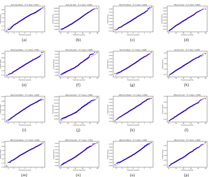
Fig. 9 (a) Shows the precision-recall curves of the measure Fbas defined in [31]. (b) Shows the precision-recall curves of

the measure Fopas defined in [31]. ‘dPRcut Multi’ and ‘dNcut Multi’ indicate the multiscale versions of PRcut and Ncut

respectively. (c) Scatter plot of optimal Fbmeasure on individual images between PRcut and Ncut. (c) Scatter plot of optimal

Fopmeasure on individual images between PRcut and Ncut. (e) Scatter plot of optimal Fbmeasure on individual images

between dPRcut and dNcut. (f) Scatter plot of optimal Fopmeasure on individual images between dPRcut and dNcut. Observe

from (c)-(f) that there is no major difference in accuracy between PRcut and Ncut measures. All results are calculated on BSDS500 dataset with the MCG algorithm, using either a NCut or a PRCut step.

Table 2 Table indicating the average times and accuracy of Ratio cut and Power Ratio cut on hyperspectral image data. The timing is reported in seconds. The accuracy is measured by (37).

Data Process

Time

Rcut PRcut

Time Accuracy Time Accuracy

Ratio = 0.7 Pavia University 129.33 95.15 0.70 27.38 0.74 Pavia Center 530.95 435.01 0.76 91.38 0.77 Salinas 142.59 94.27 0.28 24.92 0.71 Ratio = 0.8 Pavia University 194.14 151.00 0.72 34.06 0.78 Pavia Center 623.74 535.79 0.78 104.46 0.78 Salinas 202.98 139.31 0.36 26.88 0.74 Ratio = 0.9 Pavia University 279.42 163.66 0.75 40.71 0.76 Pavia Center 830.18 633.638 0.79 115.09 0.79 Salinas 271.56 170.28 0.43 31.63 0.78

Ncut PRcut dNcut dPRcut

2 4 6 8 10 12 Tim e ( in se c) (a)

Fig. 10 Box plot of the total time taken by various meth-ods. The time is on Y-axis and is measured in seconds. The time taken is calculated from the input to the final segmented output obtained by MCG on the BSDS500 dataset. Based on average values, observe that MCG using PRcut is 2.23 times faster than MCG using Ncut and MCG using dPRcut is 1.07 times faster than MCG using dNcut. However, consid-ering just the spectral clustconsid-ering step, dPRcut is 1.5-2 times faster depending on the size of the image. Since the images in BSDS500 are small the difference between MCG using dPRcut and MCG using dNcut is not visible.

we have considered three ratios -0.7, 0.8, 0.9, of their

sizes. Each experiment was repeated10 times and have

taken the average. Also, the datasets were over seg-mented and the accuracy is calculated by assuming that each cluster is labelled with the largest groundtruth

label. That is, let C = {Ci} be classes obtained by

clustering and let C∗= {C∗

i} indicate the groundtruth

classes. Let N(Ci, Cj∗) be the number of pixels labelled

Ci and Cj∗. The accuracy is then given by

accuracy(C, C∗_{) =}

P

i(maxjN(Ci, C∗j))

Total number of pixels (37)

The timing is measured in seconds. All experiments are done on Intel(R) Xeon(R) CPU E5620 at 2.40GHz with

RAM size of16 GigaBytes.

(a) (b) (c)

(d) (e) (f)

Fig. 11 Top row: Groundtruth images of Pavia Center, Pavia University and Salinas hyperspectral images. Bottom row: Results using PRcut of Pavia Center, Pavia University and Salinas hyperspectral images

An example of the results obtained of the PRcut on subsets of these images and their groundtruth is shown in figure 11. Average of accuracy and times for each of the methods is shown in table 2. Scatter plots of accuracy and times are also plotted in figure 12. It is easy to see from the table that PRcut is faster and gives better accuracy than ratio cuts (or at least equal).

5.5 High dimensional data

Another characteristic of the data is its dimensionality. In high dimensions, due to the curse of dimensionality [5, 19], it is difficult to measure the distances accurately and hence difficult to construct an edge weighted graph. The distance between points become unreliable in higher dimensions. Thus spectral clustering cannot be directly applied for clustering high dimensional data. Usually a preprocessing step is applied to the data to reduce the

Table 3 Table indicating the average times and accuracy of Ratio cut and Power Ratio cut on MNIST dataset. The timing is reported in seconds. The accuracy is measured by (37). ARI indicates Adjusted Rand Index [20], and AMI indicates Adjusted Mutual Information [37]. Data Size Process Time Rcut PRcut

Time Accuracy ARI AMI Time Accuracy ARI AMI

Dim = 10 4318 0.56 2.03 0.54 0.40 0.52 1.33 0.54 0.40 0.51 8489 1.29 15.36 0.56 0.42 0.54 7.48 0.56 0.42 0.54 12634 2.17 33.61 0.56 0.43 0.55 26.11 0.56 0.43 0.55 Dim = 15 4318 0.73 2.03 0.56 0.45 0.57 1.38 0.56 0.45 0.57 8489 1.97 12.52 0.57 0.46 0.59 7.90 0.57 0.47 0.59 12634 3.18 36.13 0.58 0.49 0.61 25.49 0.58 0.49 0.61 Dim = 20 4318 0.94 2.86 0.57 0.46 0.58 1.87 0.57 0.46 0.58 8489 2.96 11.96 0.58 0.49 0.61 9.84 0.58 0.49 0.61 12634 4.34 32.66 0.59 0.51 0.63 24.23 0.59 0.51 0.63 0.3 0.4 0.5 0.6 0.7 0.8

Normalized cut (accuracy) 0.3 0.4 0.5 0.6 0.7 0.8

Power Ratio cut (accuracy)

x0.7 x0.8 x0.9 (a) 1 2 3 4 5 6 Number of pixels in 10^5 0 100 200 300 400 500 600 700

Time (in sec)

Normalized cut Power Ratio cut

(b)

Fig. 12 (a) Scatter plot of the accuracy of normalized cuts vs power ratio cuts on hyperspectral image data. The red line indicates the line x = y. As one can see, all the points lie above or on the line x == y. Hence power ratio cut results are better than normalized cuts (or at least equal). (b) Plots of executing times vs the number of pixels in the image. It is easy to observe that PRcut scales much better compared to normalized cuts.

dimension, such as principal component analysis (PCA). The reduced data is then used for further processing.

Here the MNIST dataset [24] is used to experiment with high dimensions. The number of data points are 42000 and each data point has a dimension of 784. The

dataset if first processed with PCA to reduce the dimen-sionality. Figure 13 shows the results on the selected classes. Table 3 shows the results obtained with PRcut and spectral clustering on randomized samples of the datasets, with varying dimension. It is clear from these results that PRcut is faster than Rcut while preserving the precision of the results.

6 Conclusion

To summarize, we have proposed a faster alternative to the spectral clustering - Power Ratio cut or PRcut. This was obtained by considering a Γ −limit of the spectral clustering. Intuitively PRcut uses maximum spanning tree to reduce the size of the dataset and then solves the appropriate eigenvalue problem. This results in a much faster algorithm than spectral clustering. Also, by considering a Γ −limit several good properties of spectral clustering such as - penalizing unequal cluster distribution, ability to detect non-convex clusters is preserved. PRcut is compared with both MST-based clustering and spectral clustering considering several toy examples. Its efficiency as an alternate to Ncut is exhibited by suitably replacing Ncut in the MCG pipeline with PRcut and comparing the results on BSDS. Results of comparison with Ncut on hyperspectral image datasets are also provided. The code to generate the results in this paper is available at [7].

Note that, in this article we have considered a Γ −limit of the ratio cut. One can similarly probe the question of - "Γ −limit of normalized cut". It is relatively easy to extend the algorithm 4 replacing ratio-cut with normal-ized cut. However, the solutions to the normalnormal-ized cut problem need not belong to a bounded set as p → ∞. Hence the theory developed here must extended to in-corporate normalized cuts. This is a direction of future research.

(a)

(b)

(c)

Fig. 13 Results obtained on selected classes of the MNIST dataset. (a) Average of the groundtruth classes. (b) Average of clusters obtained by Rcut (c) Average of clusters obtained by PRcut.This figure provides a visual confirmation that the results obtained by both PRcut and Rcut are the same.

7 Appendix

Proof of Theorem 3

Proof We first show that any matrix H of the form AKY is a solution to (7). We have

T r((AKY )t_{L(AKY )) = T r(Y}t_(AK)t_{L(AK)Y )}

= T r((AK)t_L(AK))

= T r(Kt_(At_LA)K)

since Y is an orthogonal matrix. Now, AtLA is of the

form     λ1 0 · · · 0 0 λ2 · · · 0 0 · · · 0 0 0 · · · λm     So, we have T r(Kt(AtLA)K) = λ1+ λ2+ · · · + λl1+ λ(m)T r(X t_IX ) = λ1+ λ2+ · · · + λm = min T r(Ht_LH)

Since, the minimum value of T r(Ht_{LH) is equal to}

λ1+ λ2+ · · · + λm [25]. To show the other side, note

that the set of all the solutions of (7) is

{H ∈ Rn×m_{| T r(H}t_{LH) = λ}

1+ λ2+ · · · + λm}

Let A= [e1, e2, · · · en], i.e the matrix obtained by

stack-ing all the eigenvectors of L in columns. Then any H

can be written as AZ where ZtZ= I. Now, note that

since {λ1, λ2, · · · , λn} can be arbitrary, we need to have

that

Zij = 0 if λi> λ(m).

Thus we can ignore the lower part of matrix Z. If A=

[[e1, e2, · · · el]], then we have that H is of the form AZ

where Z is a l × m matrix such that ZtZ= I. Now let,

Z=Zl1,l1 Zl1,m−l1

Zl2,l1 Zl2,m−l1 

Also, note that AtLA is of the form     λ1 0 · · · 0 0 λ2 · · · 0 0 · · · 0 0 0 · · · λl    

Since Z should satisfy T r(Zt_At_{LAZ) = T r(H}t_{LH) =}

λ1+ λ2+ · · · + λm, we need to have that Zl1,l1 is full

rank, and Zt

l1,l1Zl1,l1= I. Hence Z must be of the form

KY where K is a matrix of the form (26) and Y is any orthogonal matrix. Hence all the solutions to (7) must be of the form AKY .

Proof of lemma 1

Proof One side follows from the relation

H(M(H0)) ⊇ H0

For the other side, let H be some matrix which spans

the same subspace as bH = AkKY . Then there exists

an orthogonal matrix Q such that HQ = bH. Hence

H = bHQt_{= A}

kKY Qt. This is still in the form AkKY

where Y is some orthogonal matrix.

Proof of Proposition 2

Proof To prove (a), note that since Ci is a connected

component of G≥wj, it is also a union of connected

components of G≥wi for all i >= j. Also, we know that

if L denotes a Laplacian of the graph, then L1Ci = 0

if Ci is a connected component in the graph. Hence

proved.

Since (a) is true, we know that C is a solution to (25) at level j. Thus all matrices of the form CY are

solutions. Now, since T r(Ct_L

iC) = 0 for all i >= j, any

vector c belonging to the column space of the solution

must satisfy ct_L

ic= 0 for all i >= j. This implies that

c belongs to the column space of the 0 eigenvectors,

which are indicators of connected components. Hence c must belong to the column space of the indicators

of connected components for each Gi, i >= j. This

implies that c belongs to the column space of indicators

of connected components of G≥wj, and hence belongs to

the column space of C. Hence proved.

Proof of theorem 2

Proof For the sake of simplicity, we consider x to be a 1d vector. Recall that

Q(p)(x) = T r(xt_L(p)_{x) (38)}

such that xtx= 1 and xt_{1= 0. We refer to this domain}

as d.

Now, assume that ˆx is a point belonging to M1. We

now show thatx is also a limit point. From [25],ˆ

kQ(p)_{(ˆx) − min}

x∈dQ

(p)_{(x)k → 0 as p → ∞ (39)}

On the other hand, consider a ball around x, B(ˆˆ x, ).

Then, min y∈B(0,)Q (p)_{(ˆx+ y) = ˆx}t_L(p)_{xˆ+ 2ˆx}t_L(p)_{y+ y}t_L(p)_{y (40)} Taking y= −ˆx, min y∈B(0,)Q (p) (ˆx+ y) ≤ ˆxtL(p)x(1 − 2 + ˆ 2) (41)

From (39) and (41), for p large enough, min

y∈B(0,)

Q(p)(ˆx+ y) ≤ min

x∈d

Q(p)(x) (42)

In other words, for every  ball aroundx, there exists aˆ

minimizer of Q(p)_{(x). Hence, ˆx is a limit point.}

Checking normality for t-test in Table 1

To obtain p-values in table 1 we have assumed (a)

nor-mality of samples means and (b) χ2for sample variances.

Note that these assumptions are sufficient to perform the t-test. Here, we verify these assumptions empirically.

To verify these assumptions, using bootstrap

tech-nique, we generate several samples of size30. On these

subsamples, sample means and variances are computed. Then using probability plots we empirically verify the

distribution to be normal and χ2 _{respectively. Figure 14}

show the probability plots and the R2values for various

quantitites.

Acknowledgements AC and SD would like to thank In-dian Statistical Institute. LN would like to acknowledge the funding received from - 15-CE40-0006 CoMeDiC, ANR-14-CE27-0001 GRAPHSIP research grants and Programme d’Investissements d’Avenir (LabEx BEZOUT ANR-10-LABX-58). BSDS would like to acknowledge the support received from the Science and Engineering Research Board (SERB) of the Department of Science and Technology (DST) with the grant number EMR/2015/000853, and the Indian Space Research Organization (ISRO) with the grant number ISRO/SSPO/Ch-1/2016-17.

References

1. scikit-learn datasets. http://scikit-learn.org/

stable/modules/generated/sklearn.datasets.make$\ _$circles.html. Accessed: 2017-12-12

−3 −2 −1 0 1 2 3 Theoretical quantiles 0.70 0.72 0.74 0.76 0.78 0.80 O rd er ed V al ue s

Ncut-Fo (Mean) - R^2 Value : 0.9973

(a) 10 20 30 40 50 60 Theoretical quantiles 0.0025 0.0050 0.0075 0.0100 0.0125 0.0150 0.0175 0.0200 O rd er ed V al ue s

Ncut-Fop (Var) - R^2 Value : 0.9983

(b) −3 −2 −1 0 1 2 3 Theoretical uantiles 0.275 0.300 0.325 0.350 0.375 0.400 0.425 0.450 O rd er ed V al ue s

PRcut-Fb (Mean) - R^2 Value : 0.9993

(c) 10 20 30 40 50 60 Theoretical quantiles 0.010 0.015 0.020 0.025 0.030 0.035 0.040 0.045 O rd er ed V al ue s

PRcut-Fb (Var) - R^2 Value : 0.9993

(d) −3 −2 −1 0 1 2 3 Theoretical quantiles 0.72 0.74 0.76 0.78 0.80 0.82 O rd er ed V al ue s

PRcut-Fo (Mean) - R^2 Value : 0.9991

(e) 10 20 30 40 50 60 Theoretical quantiles 0.002 0.004 0.006 0.008 0.010 0.012 0.014 0.016 0.018 O rd er ed V al ue s

PRcut-Fop (Var) - R^2 Value : 0.9908

(f) −3 −2 −1 0 1 2 3 Theoretical quantiles 0.300 0.325 0.350 0.375 0.400 0.425 0.450 0.475 O rd er ed V al ue s

Ncut-Fb (Mean) - R^2 Value : 0.9988

(g) 10 20 30 40 50 60 Theoretical quantiles 0.01 0.02 0.03 0.04 0.05 O rd er ed V al ue s

Ncut-Fb (Var) - R^2 Value : 0.9993

(h) −3 −2 −1 0 1 2 3 Theoretical quantiles 0.72 0.74 0.76 0.78 0.80 0.82 O rd er ed V al ue s

dNcut-Fo (Mean) - R^2 Value : 0.9982

(i) 10 20 30 40 50 60 Theoretical quantiles 0.0025 0.0050 0.0075 0.0100 0.0125 0.0150 0.0175 0.0200 O rd er ed V al ue s

dNcut-Fop (Var) - R^2 Value : 0.9885

(j) −3 −2 −1 0 1 2 3 Theoretical quantiles 0.275 0.300 0.325 0.350 0.375 0.400 0.425 0.450 O rd er ed V al ue s

dPRcut-Fb (Mean) - R^2 Value : 0.9996

(k) 10 20 30 40 50 60 Theoretical quantiles 0.01 0.02 0.03 0.04 0.05 O rd er ed V al ue s

dPRcut-Fb (Var) - R^2 Value : 0.9995

(l) −3 −2 −1 0 1 2 3 Theoretical quantiles 0.70 0.72 0.74 0.76 0.78 0.80 0.82 O rd er ed V al ue s

dPRcut-Fo (Mean) - R^2 Value : 0.9981

(m) 10 20 30 40 50 60 Theoretical quantiles 0.002 0.004 0.006 0.008 0.010 0.012 0.014 0.016 O rd er ed V al ue s

dPRcut-Fop (Var) - R^2 Value : 0.9972

(n) −3 −2 −1 0 1 2 3 Theoretical quantiles 0.300 0.325 0.350 0.375 0.400 0.425 0.450 0.475 O rd er ed V al ue s

dNcut-Fb (Mean) - R^2 Value : 0.9966

(o) 10 20 30 40 50 60 Theoretical quantiles 0.01 0.02 0.03 0.04 0.05 O rd er ed V al ue s

dNcut-Fb (Var) - R^2 Value : 0.9982

(p)

Fig. 14 Probability plot of sample data against the quantiles of a specified distribution - Normal for sample means and χ2_for

sample variance. The plots are generated using bootstrap samples of size 30. The data consists of means and variances of the

measures Fopand Fbof the methods PRcut, dPRcut, Ncut, dNcut. Figure titles at the top of each plot indicate the values

being plotted along with the R2_{values of the fit.}

2. scikit-learn datasets. http://scikit-learn.org/stable/ modules/generated/sklearn.datasets.make$\_$blobs. html. Accessed: 2017-12-12

3. Arbelaez, P.: Boundary extraction in natural images us-ing ultrametric contour maps. In: Computer Vision and Pattern Recognition Workshop, 2006. CVPRW’06. Con-ference on, pp. 182–182. IEEE (2006)

4. Arbelaez, P., Maire, M., Fowlkes, C., Malik, J.: Contour detection and hierarchical image segmentation. IEEE transactions on pattern analysis and machine intelligence 33(5), 898–916 (2011)

5. Bellman, R.E.: Adaptive control processes: a guided tour. Princeton university press (2015)

6. Braides, A.: Gamma-convergence for Beginners, vol. 22. Clarendon Press (2002)

7. Challa, A.: Power spectral clustering. https://github. com/ac20/Power-Spectral-Clustering (2018)

8. Challa, A., Danda, S., Daya Sagar, B.S., Najman, L.: An Introduction to Gamma-Convergence for Spectral

Clus-tering, pp. 185–196. Springer International Publishing, Cham (2017). DOI 10.1007/978-3-319-66272-5_16. URL https://doi.org/10.1007/978-3-319-66272-5_16 9. Challa, A., Danda, S., Daya Sagar, B.S., Najman, L.:

Power Spectral Clustering on Hyperspectral Data. In: International Geoscience and Remote Sensing Symposium. IEEE, Forth Worth, United States (2017). URL https: //hal.archives-ouvertes.fr/hal-01484896

10. Chen, J., Fang, H.r., Saad, Y.: Fast approximate knn graph construction for high dimensional data via recursive lanczos bisection. Journal of Machine Learning Research 10(Sep), 1989–2012 (2009)

11. Couprie, C., Grady, L., Najman, L., Talbot, H.: Power watershed: A unifying graph-based optimization frame-work. IEEE transactions on pattern analysis and machine intelligence 33(7), 1384–1399 (2011)

12. Cousty, J., Bertrand, G., Najman, L., Couprie, M.: Wa-tershed cuts: Minimum spanning forests and the drop of