HAL Id: hal-01824205
https://hal.inria.fr/hal-01824205v3
Submitted on 18 Jan 2019
HAL is a multi-disciplinary open access
archive for the deposit and dissemination of
sci-entific research documents, whether they are
pub-lished or not. The documents may come from
teaching and research institutions in France or
abroad, or from public or private research centers.
L’archive ouverte pluridisciplinaire HAL, est
destinée au dépôt et à la diffusion de documents
scientifiques de niveau recherche, publiés ou non,
émanant des établissements d’enseignement et de
recherche français ou étrangers, des laboratoires
publics ou privés.
Benchmarking functional connectome-based predictive
models for resting-state fMRI
Kamalaker Dadi, Mehdi Rahim, Alexandre Abraham, Darya Chyzhyk,
Michael Milham, Bertrand Thirion, Gaël Varoquaux
To cite this version:
Kamalaker Dadi, Mehdi Rahim, Alexandre Abraham, Darya Chyzhyk, Michael Milham, et al..
Bench-marking functional connectome-based predictive models for resting-state fMRI. NeuroImage, Elsevier,
2019, pp.115-134. �10.1016/j.neuroimage.2019.02.062�. �hal-01824205v3�
Benchmarking functional connectome-based predictive models for resting-state fMRI
Kamalaker Dadia,b,∗, Mehdi Rahima,b, Alexandre Abrahama,b, Darya Chyzhyka,b,c, Michael Milhamc, Bertrand
Thiriona,b, Ga¨el Varoquauxa,b, for the Alzheimer’s Disease Neuroimaging Initiatived aParietal project-team, INRIA Saclay-ˆıle de France, France
bCEA/Neurospin bˆat 145, 91191 Gif-Sur-Yvette, France
cCenter for the Developing Brain Child Mind Institute, Center for Biomedical Imaging and Neuromodulation, Nathan S. Kline Institute
for Psychiatric Research, USA
dOne of the dataset used in preparation of this article were obtained from the Alzheimer’s Disease Neuroimaging Initiative (ADNI)
database (adni.loni.usc.edu). As such, the investigators within the ADNI contributed to the design and implementation of ADNI and/or provided data but did not participate in analysis or writing of this report. A complete listing of ADNI investigators can be found at:
http://adni.loni.usc.edu/wp-content/uploads/how to apply/ADNI Acknowledgement List.pdf
Abstract
Functional connectomes reveal biomarkers of individual psychological or clinical traits. However, there is great variabil-ity in the analytic pipelines typically used to derive them from rest-fMRI cohorts. Here, we consider a specific type of studies, using predictive models on the edge weights of functional connectomes, for which we highlight the best modeling choices. We systematically study the prediction performances of models in 6 different cohorts and a total of 2 000 individ-uals, encompassing neuro-degenerative (Alzheimer’s, Post-traumatic stress disorder), neuro-psychiatric (Schizophrenia, Autism), drug impact (Cannabis use) clinical settings and psychological trait (fluid intelligence). The typical predic-tion procedure from rest-fMRI consists of three main steps: defining brain regions, representing the interacpredic-tions, and supervised learning. For each step we benchmark typical choices: 8 different ways of defining regions –either pre-defined or generated from the rest-fMRI data– 3 measures to build functional connectomes from the extracted time-series, and 10 classification models to compare functional interactions across subjects. Our benchmarks summarize more than 240 different pipelines and outline modeling choices that show consistent prediction performances in spite of variations in the populations and sites. We find that regions defined from functional data work best; that it is beneficial to capture between-region interactions with tangent-based parametrization of covariances, a midway between correlations and par-tial correlation; and that simple linear predictors such as a logistic regression give the best predictions. Our work is a step forward to establishing reproducible imaging-based biomarkers for clinical settings.
Keywords: Resting-state fMRI; Functional connectomes; Predictive modeling; Classification; Population study
1. Introduction
Resting-state functional Magnetic Resonance Imaging (rest-fMRI), based on the analysis of brain activity with-out specific task, has become a tool of choice to probe hu-man brain function in healthy and diseased populations. As it can easily be acquired in many different individuals, rest-fMRI is a promising candidate for markers of brain function (Biswal et al., 2010; Greicius, 2008). This has lead to the rise of large-scale rest-fMRI data collections, such as the human connectome project (Van Essen et al., 2013) or ABIDE (Di Martino et al.,2014). Larger datasets bring increased statistical power (Elliott et al.,2008), and many population-imaging studies use rest-fMRI to relate brain imaging to neuropathologies or other behavior and population phenotypes (Miller et al., 2016; Dubois and Adolphs,2016). These efforts build biomarkers from rest-fMRI with predictive models (Woo et al.,2017).
∗Corresponding author
A functional connectome – characterizing the network structure of the brain (Sporns et al., 2005)– can be ex-tracted from functional interactions in rest-fMRI data (Varoquaux and Craddock,2013). The weights of the cor-responding brain functional connectome are used to char-acterize individual subjects behavior, cognition, and men-tal health (Craddock et al., 2009; Richiardi et al., 2010; Milazzo et al.,2014;Smith et al.,2015;Miller et al.,2016; Colclough et al., 2017; Dubois et al., 2018), aging (Liem et al., 2017) as well as brain pathologies (Drysdale et al., 2016;Abraham et al.,2017;Ng et al.,2017).
Machine-learning pipelines are key to turning func-tional connectomes into biomarkers that predict the phe-notype of interest (Woo et al.,2017). On rest-fMRI, such a pipeline typically comprises of 3 crucial steps as depicted in Figure 1, linking functional connectomes to the target phe-notype (Varoquaux and Craddock,2013;Craddock et al., 2015). Yet, there exist many variations of this prototypical pipeline, even for classification from edge-weights of brain functional connectomes, as revealed by reviews of the field
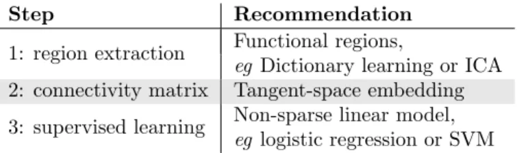
Figure 1: Functional connectome-prediction pipeline with three main steps: 1) definition of brain regions (ROIs) from rest-fMRI images or us-ing already defined reference atlases, 2) quantifying functional interactions from time series signals extracted from these ROIs and 3) comparisons of functional interactions across sub-jects using supervised learning.
RS-fMRI
Diagnosis
Connectivity
Parameterization Supervised Learning Defining Brain
ROIs
1 2 3
(Wolfers et al.,2015;Arbabshirani et al.,2017;Brown and Hamarneh, 2016). These various choices have a sizable impact on the accuracy of population studies, and are sel-dom discussed (Carp, 2012). The cost of such analytical variation is twofold. First, it puts the burden on the prac-titioner to explore many options and make choices with-out systematic guidance. Second, methods variations cre-ate researchers degrees of freedom (Simmons et al.,2011) that can compromise the measure of the prediction accu-racy of biomarkers (Varoquaux,2017). Guidelines on opti-mal modeling choices are thus of great value for rest-fMRI biomarker research.
Here, we perform a systematic benchmark of common choices for the different steps of the functional connectome-based classification pipeline. To outline the preferable strategies, we analyze the prediction accuracy across 6 dif-ferent cohorts, with difdif-ferent clinical questions and one psychological trait, different sample sizes, and prediction problems of different difficulties. While best model choice may vary depending on the prediction task, our bench-marks outline some trends. Specifically, we explore the following analytical choices:
• How should nodes be chosen: via pre-defined atlases, or data-driven approaches? How many nodes are needed for brain-imaging based diagnosis? Should nodes be dis-tributed brain networks or regions of interest (ROIs)? • How should weights of brain functional connectomes be
represented: via correlations, partial correlation, or more complex models capturing the geometry of covariance matrices?
• What classifiers should be used for machine learning on weights of brain functional connectomes? Should linear or linear models be preferred? Should sparse or non-sparse models be used? With or without feature selec-tion?
Besides these main questions, we did additional experi-ments on preprocessing strategies —studying the effect of band-pass filtering and global signal regression— and on covariance estimators, by comparing sparsity-inducing to classical shrinkage.
The paper is organized as follows: we first review cur-rent practices and methods used to-date for prediction of psychiatric diseases from weights of brain functional con-nectomes. Then, we present the different choices that we benchmark for the steps of classification pipelines and de-scribe these methods. Finally, we report our experimental
results and the trends that they reveal.
2. Methods: functional connectome-classification pipeline
Figure 1 shows the standard rest-fMRI classification pipeline that we consider.
2.1. A brief review of current practices: functional connectome-based predictive methods
We first survey methods used for prediction studies based on three extensive reviews: Wolfers et al. (2015); Arbabshirani et al.(2017);Brown and Hamarneh (2016). From these reviews, 27 studies used rest-fMRI and gave good classification scores. Below, we briefly outline the choices in the different pipeline step used (seeTable A2in the appendix for the full list).
Definition of brain ROIs. Studies define ROIs to extract signals with a variety of approaches:
• balls1of radius varying from 5mm to 10mm centered at
coordinates from the literature (Dosenbach et al.,2010; Power et al., 2011);
• reference anatomical atlases such as AAL ( Tzourio-Mazoyer et al., 2002), sulci-based atlases (Perrot et al., 2009;Desikan et al.,2006), or connectivity-based cortical landmarks (Zhu et al.,2013);
• data-driven approaches based on k-means or Ward clus-tering, as well as Independent Component Analysis (ICA) approaches (Calhoun et al., 2001;Beckmann and Smith, 2004) or dictionary learning (Abraham et al., 2013).
The number of nodes used was typically around 100, but ranged from dozens to several hundreds.
Representation of brain functional connectomes. Studies define functional interactions from second-order statis-tics –based on signal covariance– using Pearson’s corre-lation or partial correcorre-lations estimated mostly either with the maximum-likelihood formula for the covariance or the Ledoit-Wolf shrinkage covariance estimator (Ledoit and Wolf, 2004; Varoquaux and Craddock, 2013; Brier et al., 2015). Partial correlation between nodes is useful to rule
1We used the term ball rather a sphere. From a mathematical
out indirect effects in the correlation structure, but calls for shrunk estimates (Smith et al.,2011;Varoquaux et al., 2010b). Mathematical arguments have also led to repre-sentations tailored to the manifold-structure of covariance matrices (Varoquaux et al.,2010a;Ng et al.,2014;Dodero et al., 2015; Colclough et al., 2017). We benchmark the simplest of these, a tangent representation of the mani-fold which underlies the more complex developments (see Appendix Afor a quick introduction to this formalism). Classifiers used for prediction. Many different classifiers have been used, whether linear or non-linear, sparse or non-sparse, optionally with prior feature selection. See Table A2 for the comprehensive list of classifiers used in these studies.
Finally, beyond the prototypical pipeline exposed above, some studies employ complex-graph network mod-eling approaches –e.g. network modularity or centrality (Rubinov and Sporns,2011)– (Wolfers et al.,2015; Arbab-shirani et al., 2017; Brown and Hamarneh, 2016) These approaches are seldom combined with supervised learning. Indeed, graph-theory metrics capture well global aspects of brain connectivity, but do not lend themselves well to tuning to connections in specific subnetworks (Hallquist and Hillary, 2018). Here, we focus on machine-learning methods that extract discriminant connections; as such we do not study graph-theoretical approaches.
The current practice is very diverse, without standard modeling choices. To open the way toward informed deci-sions, we explore popular variants of the classic machine-learning pipeline to predict on connectomes. We measure the impact of choices at each step on prediction for diverse targets across multiple datasets. We detail below the spe-cific modeling choices included in our benchmarks. 2.2. Definition of brain regions of interest (ROIs)
For functional connectomes, the hypothesis is that the definition of ROIs should capture well the relevant func-tional units (Smith et al.,2011). We study both anatom-ically and functionally defined reference brain atlases, as well as data-driven methods that define ROIs from the data at hand. ROI selection is a difficult choice, as the optimal may vary for different conditions or pathologies. A selection of pre-defined atlases. We consider four stan-dard atlases, of which two are structural atlases: i) Automated Anatomical Labeling (AAL) (Tzourio-Mazoyer et al., 2002), a structural atlas with 116 ROIs defined from the anatomy of a reference subject, ii) Har-vard Oxford (Desikan et al.,2006), a probabilistic atlas of anatomical structures, contains of 48 cortical & 11 sub-cortical ROIs in each hemisphere, ie 118 ROIs in total. We also include two functional atlases: iii) Bootstrap Anal-ysis of Stable Clusters (BASC) (Bellec et al., 2010),
a multi-scale functional atlas built with clustering on rest-fMRI, coming with different {36, 64, 122, 197, 325, 444} numbers of ROIs; iv) Power, a coordinate-based atlas consisting of 264 coordinates used to position balls of 5mm radius (Power et al.,2011). For an additional set of bench-marks, on larger data, we use only pre-computed regions. For a pre-computed functional atlas with dictionary learn-ing, we use an atlas2 computed by Mensch et al. (2016a) with a very scalable sparse dictionary-learning algorithm on the HCP900 dataset (Van Essen et al.,2012). This algo-rithm, MODL (massive online dictionary learning), solves the `1dictionary-learning problem with an algorithm fast
on very large datasets that converges to the same solution as standard on-line solvers (Mensch et al.,2018).
A selection of data-driven methods. We consider four pop-ular data-driven methods to extract brain ROIs from in-trinsic brain activity (Yeo et al.,2011;Kahnt et al.,2012; Thirion et al.,2014; Calhoun et al., 2001;Beckmann and Smith, 2004; Abraham et al., 2013). We choose to define ROIs using two clustering methods: i) K-Means (Hastie et al., 2009), and ii) hierarchical agglomerative cluster-ing uscluster-ing Wards algorithm (Ward, 1963) with spatial connectivity constraints (Michel et al.,2012); and two lin-ear decomposition methods: iii) Canonical Indepen-dent Component Analysis (GroupICA or CanICA) (Varoquaux et al.,2010c), iv) Dictionary Learning - `1
(DictLearn) (Mensch et al.,2016b).
Dimension selection in data-driven atlases. For clustering methods, we extract brain atlases with a varying number of ROIs in dim = {40, 60, 80, 100, 120, 150, 200, 300}. With linear decomposition methods i.e. CanICA and DictLearn, we explore the following number of compo-nents: dim = {40, 60, 80, 100, 120}3.
For each data-driven method, we learn brain ROIs on the training set only, to avoid possible overfit (Abraham et al., 2017). In a cross-validation loop, for each split, we define the brain ROIs on a training set and use the atlases to learn connectivity patterns for prediction. We also applied additional Gaussian smoothing of 6mm on preprocessed rest-fMRI datasets for all data-driven meth-ods prior to learning brain ROIs to enhance the region extraction step.
Nodes formed local regions or distributed networks?. Cur-rent practices in functional connectomics includes defining nodes as local regions of the brain (Shirer et al., 2012;
2Pre-computed sparse dictionaries with the MODL approach of
Mensch et al.(2016a) are available from https://team.inria.fr/ parietal/files/2018/10/MODL_rois.zip
3We also investigated higher dimensionality (150, 200 and 300)
on some of the datasets, but could not do a systematic study above 300 because of high computational costs. These preliminary results showed no improvements in prediction accuracy compared to lower dimensionalities. It should be noted that the resulting components typically encompass several brain regions, which explains the dimen-sion difference.
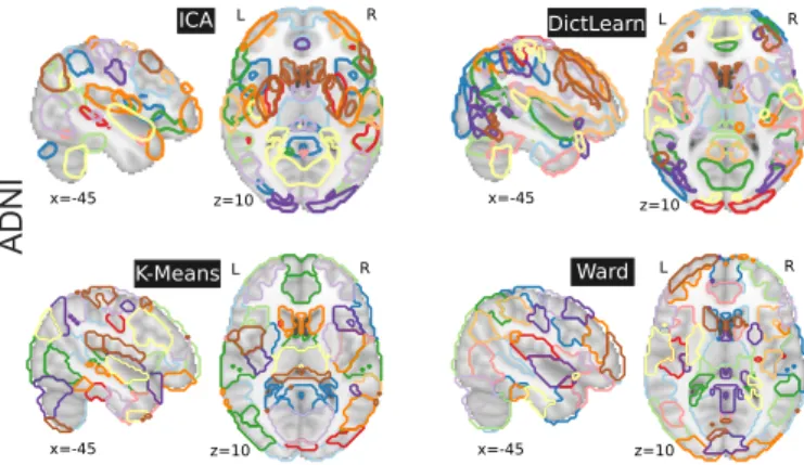
L L R R L L R ICA DictLearn x=-45 K-Means Ward R x=-45 z=10 z=10 x=-45 z=10 x=-45 z=10
Figure 2: Brain regions extracted with ICA, DictLearn, KMeans, and Ward For ICA and dictionary learning, the dimen-sionality is of 80 and 60 resting-state networks – which are then bro-ken up into more regions – yielding 150 regions, and 120 for KMeans and Ward clustering. Colors are arbitrary.
Craddock et al., 2012), or as full distributed functional networks that may include several regions (Smith et al., 2015; Yeo et al., 2011). We consider both approaches: using the distributed networks, or breaking them up in regions with a segmentation step to separate out regions (Abraham et al., 2014a). For example, a bi-hemispheric brain networks is separated into regions, one in each hemi-sphere.
We use a Random-Walker based extraction of re-gions from the brain networks obtained by CanICA and DictLearn as proposed in Abraham et al. (2014a). By contrast, for K-Means and BASC, we simply break out clusters in their connected components. During this pro-cedure, we remove spurious regions of size < 1500mm3. Figure 2shows an example of the set of brain regions ob-tained from the various data-driven methods on the ADNI rest-fMRI data.
2.3. Connectivity parametrization
We extract representative time series for each node. For signal extraction, we explored several denoising strate-gies to account for non-neural artifacts: with or without low-pass filtering or global signal mean regression (details in Appendix B). To estimate functional connectomes effi-ciently, we use the Ledoit-Wolf regularized shrinkage esti-mator (Ledoit and Wolf,2004;Varoquaux and Craddock, 2013;Brier et al.,2015), which gives a closed form expres-sion for the shrinkage parameter. This estimator yields well-conditioned estimators despite the variation in length of time series across rest-fMRI datasets. We also explored non-regularized and sparse estimator for the covariance (see Appendix H.2). With this covariance structure, we study three different parametrizations of functional inter-actions: full correlation, partial correlation (Smith et al.,2011;Varoquaux and Craddock,2013) and the tan-gent space of covariance matrices. The latter is less frequently used but has solid mathematical foundations and a variety of groups have reported good decoding
per-formances with this framework (Varoquaux et al., 2010a; Barachant et al.,2013;Ng et al.,2014;Dodero et al.,2015; Qiu et al., 2015; Rahim et al., 2017; Wong et al., 2018). We compared two variants, using as a reference point the Euclidean mean (Varoquaux et al.,2010a) or the geometric mean (Ng et al.,2014); in both cases we rely on Nilearn im-plementation (Abraham et al.,2014b). Note that comput-ing partial correlation or tangent space require invertcomput-ing covariance matrices, hence these must be well conditioned. Non regularized covariance estimation is thus not useable for these parametrizations.
For each parametrization, we vectorize the functional connectome, using the lower triangular part of the connec-tomes matrix for classification. Additionally, on the ACPI dataset, we considered the ADHD status of the subjects as a variable of non interest and regressed it out in this second-level analysis, as we were interested in predicting the consumption of Marijuana.
2.4. Supervised learning: Classifiers
The final step of our pipeline predicts a binary phe-notypic status from connectivity features extracted from previous step. We consider several linear and non-linear classifiers for prediction i.e. both sparse and non-sparse methods. For non-linear methods, we consider Near-est Neighbors (K-NN) (Cover and Hart, 1967) with K=1 and Euclidean distance metric, Gaussian Na¨ıve Bayes (GNB) and Random Forests Classifier (RF) (Breiman, 2001). For linear classifiers we consider sparse `1 regularization4 for Support Vector Classification
(SVC), and Logistic Regression (Hastie et al., 2009). For non-sparse linear classifiers –i.e. `2regularization– we
consider Ridge classification, SVC, Logistic regres-sion. For SVC, we also considered 10% feature screening with univariate ANOVA. With regards to the regulariza-tion parameter (eg soft margin parameter in SVC), we use the default C = 1 or α = 1, which has been found to be a good default (Varoquaux et al.,2017).
3. Experimental study
To benchmark the various predictive-modeling choices, we apply the functional connectome-classification pipeline on five publicly-available rest-fMRI datasets. We study prediction from functional connectomes of various clinical outcomes –neuro-degenerative and neuro-psychiatric dis-orders, drug abuse impact, fluid intelligence. We focus on binary classification problems, predicting a phenotypic target between two groups. We use the following datasets, summarized inTable 1:
1. COBRE, Center for Biomedical Research Excel-lence5, comprising rest-fMRI data to study schizophre-nia and bipolar disorder (Calhoun et al., 2012). We 4We also included Lasso as another choice of classifier in the
pipeline. We observed significantly low prediction performance.
5
focus on predicting schizophrenia diagnosis versus nor-mal control.
2. ADNI, the Alzheimer’s Disease Neuroimaging Ini-tiative6 database studies neuro-degenerative diseases (Mueller et al., 2005). We focus on using rest-fMRI to discriminate individuals with Mild Cognitive Impairment (MCI) from individuals diagnosed with Alzheimer’s Disease (AD).
3. ADNIDOD, funded by the US Department of De-fense (DoD) to study brain aging in Vietnam War Veterans7, includes rest-fMRI data of individuals with post-traumatic stress disorders (PTSD) or brain trau-matic injuries. We focus on discriminating PTSD con-dition from normal controls.
4. ACPI, Addiction Connectome Preprocessed Initia-tive8, a longitudinal study to investigate the effect of cannabis use among adults with a childhood diagnosis of ADHD. In particular we use readily-preprocessed rest-fMRI data from Multimodal treatment study of Attention Deficit Hyperactivity Disorder (MTA). We attempt to discriminate whether individuals have con-sumed marijuana or not.
5. ABIDE, Autism Brain Imaging Data Exchange database investigates the neural basis of autism (Di Martino et al., 2014). We use the data from Preprocessed Connectome Project (Craddock et al., 2013) to discriminate individuals from Autism Spec-trum Disorder from normal controls.
6. HCP,9 Human Connectome Project contains imag-ing and behavioral data of healthy subjects (Van Es-sen et al.,2013). We use preprocessed rest-fMRI data from HCP900 release (Van Essen et al., 2012) to dis-criminate individuals from high IQ and low IQ. We used HCP rs-fMRI datasets to probe a different set-ting: data with longer acquisitions. Due to the data size, we limit the benchmarks here to pre-computed atlases.
3.1. rest-fMRI data processing: softwares and related Data preprocessing. We preprocess COBRE, ADNI, and ADNIDOD. We use a standard protocol that includes: motion correction, fMRI co-registration to T1-MRI, nor-malization to the MNI template using SPM1210, Gaussian
spatial smoothing (F W HM = 5mm). The SPM based preprocessing pipeline is implemented through pyprepro-cess11- Python scripts relying on Nipype interface
(Gor-golewski et al.,2011). All subjects were visually inspected 6
www.adni-info.org
7www.adni-info.org/DOD.html 8
http://fcon_1000.projects.nitrc.org/indi/ACPI/html/
9We perform some additional experiments on the Human
Connec-tome Project (HCP) data, to assess that our experimental results still hold when using high-quality datasets like HCP.
10www.fil.ion.ucl.ac.uk/spm/ 11
https://github.com/neurospin/pypreprocess
Dataset Prediction task Groups COBRE Schizophrenia vs Control 65/77
ADNI AD vs MCI 40/96
ADNIDOD PTSD vs Control 89/78 ACPI Marijuana use vs Control 62/64 ABIDE Autism vs Control 402/464
HCP High IQ vs Low IQ 213/230
Table 1: Datasets and prediction tasks, as well as the number of subjects in each group. COBRE - 142 subjects, ADNI - 136 sub-jects, ADNIDOD - 167 subsub-jects, ACPI - 126 subsub-jects, ABIDE - 866 subjects, HCP - 443. IQ represents fluid intelligence; 788 subjects had an IQ score in the HCP900 release. The acquisition parameters of each dataset are summarized inTable A3.
and excluded from the analysis if they have severe scan-ner artifacts or head movements with amplitude larger than 2mm. Since pre-processed rest-fMRI subjects from ABIDE and ACPI are available, we choose images pre-processed using C-PAC pipeline (Craddock et al.), with-out global signal regression. For ACPI, we choose linearly registered images using (Advanced Normalization Tools) ANTS and without motion scrubbing and no global signal regression. For already available preprocessed rest-fMRI subjects, we select the protocols such that it matches with the standard protocol we use. We have not done any ad-ditional preprocessing steps on ABIDE and ACPI. Exclusion criteria. We not only exclude subjects based on visual inspection of preprocessed data, but also sub-jects that do not fall into binary classification groups, eg we removed subjects who had both bipolar disorder and schizoaffective groups from COBRE samples. For HCP, we select the subjects with single session and phase encoding in a left-to-right (LR) direction. Out of these selected sub-jects, we discriminate the low IQ from the high IQ individ-uals, where the data are split in 3 according to quantiles 0.333 and 0.666, and the subjects in the middle group are excluded to make the prediction easier in a binary classifi-cation setup (seeTable 1for numbers of subjects included in the analysis).
Cross validation and error measure. We perform cross-validation (CV) by randomly shuffling and splitting each dataset over 100 folds, forming two sets of subjects: 75% for training the classifier and learning brain atlases with data-driven models and the remaining 25% for testing on unseen data (Varoquaux et al.,2017). We create stratified folds, preserving the ratio of samples between groups. For each split, we measure the Area Under the Curve (AUC) from the Receiver Operating Characteristics (ROC) curve: 1 is a perfect prediction and .5 is chance. The final pre-diction scores in AUC (> 120k scores) are used to measure the impact of various choices in our prediction pipeline outlined below in results section.
Computations and implementation. Our experimental study consists of more than 240 types of pipelines (8
at-lases × 3 connectivity measures × 10 classifiers, plus some variants such as 3 filtering options and 3 covariance es-timator options). These pipelines were run on each of 5 datasets for 100 CV folds. As a result, there are more than 500 000 pipeline fits, from the raw data to the supervised step, a heavy computational load. Technically, we rely on efficient implementations open-source scientific computing packages using Python 2.7: Nilearn v0.3 (Abraham et al., 2014b) to define brain atlases, extract representative time-series and timetime-series confounds regression, and build con-nectivity measures. All machine-learning methods used for prediction i.e., classifiers and cross-validation are imple-mented with scikit-learn v0.18.1 (Pedregosa et al.,2011). For visualization, we rely on Nilearn for brain-related fig-ures while matplotlib is used (Hunter,2007) for generating other figures.
4. Results: benchmarks of pipeline choices
We now outline which modeling choices have an impor-tant impact on predicting over diverse phenotypes from all rest-fMRI datasets.
We report inTable 2the AUC scores obtained for all rest-fMRI datasets. The scores reported in the table are simplified to the optimal choice selection at each step in the pipeline which showed significant impact. These optimal choice of steps are discussed in following sections.
Impact of methodological choices. We study the prediction score of each pipeline relative to the mean across pipelines on each fold. This relative measure discards the variance in scores due to folds or datasets. From these relative prediction scores, we study the impact of the choice of each step in the prediction pipeline: choice of classifiers, connectivity parametrizations, and brain atlases. This is a multifactorial set of choices and there are two points of view on the impact of a choice for a given step. First, the impact of the choice for one step may be considered when the other steps are optimal, or close to optimal. Second, the impact of one step may be considered for all other choices for the other steps –marginally on the choice of other steps. Empirically, the two scenario lead to similar conclusions. In the following figures, we study the first
Accuracy COBRE ADNIDOD ADNI ABIDE ACPI 5thpercentile 75.5% 69.9% 57.8% 66% 42.5% Median 86.2% 79.5% 72.5% 71.1% 55.4% 95thpercentile 95% 90.6% 84.5% 75.6% 68.7% Table 2: 5th percentile, median and 95th percentile of accu-racy scores in AUC over cross-validation folds (n = 100) for all five rest-fMRI datasets. Accuracy scores reported correspond to optimal choices in functional connectivity prediction pipeline: brain regions defined with regions using DictLearn, connectivity ma-trices parametrized by their tangent-space representation, and an `2-regularized logistic regression as a classifier, as discussed below.
Best prediction is achieved with schizophrenia vs control discrimina-tion task on COBRE dataset at 86.2% (median).
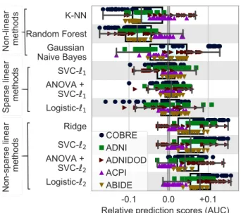
Figure 3: Impact of classifier choices on prediction accuracy, for all rest-fMRI datasets and all folds. For each classifier choice, only the top third highest performing scores are represented when varying the modeling choices for other steps in the pipeline: brain-region definition and connectivity parametrization. Figure A2gives all the data points, not limited to good choices in the overall pipeline. Overall, `2-regularized linear classifiers perform better, with a slight
lead for `2 logistic regression. The box plot gives the distribution
across folds (n=100) and datasets (denoted by markers) of predic-tion score for a given choice (classifier) relative to the mean across all choices (regions-definition and connectivity parametrizations, classi-fiers). The box displays the median and quartiles, while the whiskers give the 5thand 95thpercentiles.
situation, focusing on “good choices”: given a choice for one step, we report data for top third highest performing scores (quantiles 0.666) for the choices in the other steps. Appendix Cgives results for all scores, hence studying one choice, marginally upon the others.
4.1. Choice of classifier
Figure 3 summarizes the performances of classifiers on prediction scores for all rest-fMRI datasets. The re-sults display a certain amount of variance across folds and datasets (i.e., prediction targets). However, they show that non-sparse (`2-regularized) linear classifiers perform
better, with a slight lead for logistic-`2. Using non-linear
classifiers does not appear useful; neither does sparsity. The results in Figure 3are conditional on a good choice for the other steps of the pipeline. The marginal perfor-mances of the different choices of classifiers –i.e. cconsid-ering all other choices in the pipeline– are shown in Fig-ure A2. They show similar trends, leading to preferring `2-regularized linear classifiers.
4.2. Choice of connectivity parameterization
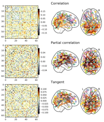
Figure 4 summarizes the impact of covariance matrix parametrization on the relative prediction scores for all rest-fMRI datasets. Tangent-space parametrization tends
Figure 4: Impact of connectivity parameterization on pre-diction accuracy, for all rest-fMRI datasets and folds. For each parametrization choice, only the top third highest performing scores are represented when varying the modeling choices for other steps in the pipeline: brain-region definition and classifier. Figure A3gives all the data points, not limited to good choices in the overall pipeline. Prediction using tangent space based connectivity parameterization displays higher accuracy with relatively lower variance than using full or partial correlation. The box displays the median and quartiles, while the whiskers give the 5thand 95thpercentiles.
to outperform full correlations or partial correlations. In-deed, it performs better on average, but also has less vari-ance across datasets (prediction targets) or folds. Re-sults are similar for simpler variant of the tangent-space parametrization relying on a simple Euclidean mean rather than the full geometric (Riemannian) –seeAppendix Afor more details. While scores inFigure 4are conditional on a good choice for other pipeline parameters,Figure A3gives results marginal to all choices. In both settings, connectiv-ity matrices built with tangent space parametrization give an improvement compared to full or partial correlations. 4.3. Choice of regions definition method
To find the preferred approaches to define brain re-gions, we proceed in two steps. First, for each method, we find the dimensionality that gives the best prediction. This holds for the BASC atlas, that comes in various dimen-sionalities, and for data-driven region-definition methods, for which we vary the dimensionality. Second, we study the prediction accuracy for each approach at the optimal dimensionality.
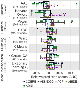
Best approach. Figure 5 summarizes the relative predic-tion performance of all choices of region-definipredic-tion meth-ods. While the systematic effects are small compared to the variance over the folds and the datasets, the general trend is that regions defined from functional data lead to better prediction than regions defined from anatomy. Using `1 dictionary learning to define regions from
rest-fMRI data appears to be the best method, closely fol-lowed by ICA, which is also based on a linear decomposi-tion model. Interestingly, BASC, an atlas pre-defined on unrelated rest-fMRI datasets using data-driven clustering
Figure 5: Impact of region-definition method on prediction accuracy, for all rest-fMRI datasets and folds. For each region-definition choice, only the top third highest performing scores are represented when varying the modeling choices for other steps in the pipeline: classifier and connectivity parametrization. Figure A4
gives all the data points, not limited to good choices in the overall pipeline. Learning atlases from rest-fMRI data tends the prediction for all tasks. By contrast anatomical atlases perform poorly over diverse tasks. The box displays the median and quartiles, while the whiskers give the 5thand 95thpercentiles.
technique, performs almost as well as the best regions-extraction method applied to the rest-fMRI data of inter-est. Unlike other pre-defined atlases, like Harvard Oxford or AAL, that lack some crucial functional regions. The BASC atlas (Bellec et al., 2010) is readily available on-line, and is thus easy to apply to data. Figure 5 shows the impact of region-definition approach conditional on good choices in the other steps of the pipeline, however studying the impact of region-definition independently of other choices (Figure A4). Both comparisons highlight that defining regions from functional data gives the best-performing pipelines, and that linear-decomposition meth-ods are to be preferred.
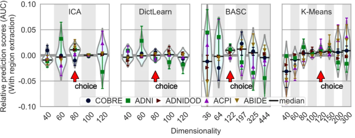
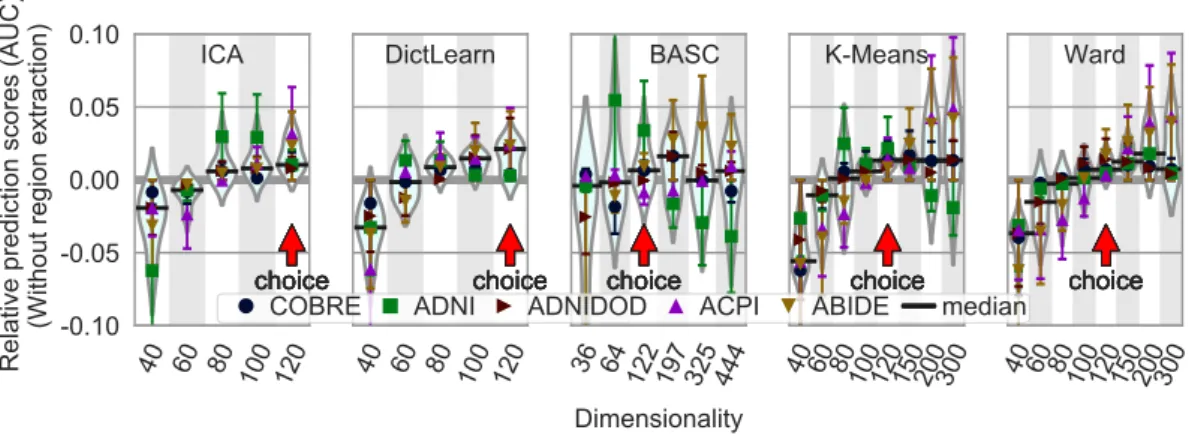
Optimal dimensionality. The choice of the best dimen-sionality for each approach paints a less clear picture (Fig-ure 6): a range of dimensionalities lead for good predic-tion for each method12. We find that there is a very soft optimum: prediction reaches a plateau as the number of extracted networks increases, and then slowly decreases for some methods. To favor the most parsimonious model, in this paper we choose to work at the lower end of the
12Note that, these curves are shown for the optimal choices found
above: an `2-penalized logistic regression as a classifier, and
Figure 6: Impact of the number of regions in atlases on prediction accuracy. The figure shows the distribution of the relative accuracy AUC scores across methods on the five rest-fMRI datasets, as a function of the number of regions. Horizontal bars (black) represent the median of the relative scores for the given number of regions. The chosen dimensionality for each method is indicated by a red arrow and was selected as the one with lowest variance in the error, and a median above zero.
plateau (red arrow on Figure 6): simpler models for bet-ter stability and statistical control. While this choice is not clear cut, the curves also suggest that, in a reasonable range, it does not have a large impact on prediction accu-racy. Note that the dimensionality here corresponds to the number of networks, these are then broken up into sepa-rate regions. We find that the typical number of regions at the optimal is around 150 (Appendix E).
Localized regions or distributed networks. Nodes of the functional connectomes may be defined from localized re-gions, or the distributed networks that naturally arise from approaches such as ICA or dictionary learning. The choice of one over the other has little impact over prediction, though there is slight, non significant, benefit to using re-gions (Figure A5).
4.4. Larger datasets and pre-computed atlases
To investigate the consistency of analytics choices for higher-quality datasets, we perform extra benchmarks in-cluding the HCP data. As this data comprises much longer time-series, we restrict our analysis to pre-computed at-lases, that alleviate computational costs. We share the resulting time-series and scripts to reproduce our analy-sis13.
Figure 7 summarizes the impact of method choice on the prediction accuracy for all six different cohorts. This experiment outline similar tradeoffs as the others: functional atlas pre-computed with dictionary learning (here MODL, from Mensch et al.(2016a)), tangent-space parametrization, and `2-regularized classifiers are
prefer-able. This experiment is not as systematic as the other, as a very large dataset like HCP would require much more
13github.com/KamalakerDadi/benchmark rsfMRI prediction
computing power to study region extraction14. Yet, even
for region-definition methods, it outlines similar trends than when tuning the regions to the data at hand. 4.5. Filtering, global signal, and covariance estimation
When extracting functional signal for connectivity modeling, there are many options to reject confounds, in-cluding temporal filtering or global signal mean regression (Fox et al.,2009;Murphy et al.,2009;Power et al.,2012). Also, to extract a structure reflecting well brain connec-tivity, it has been show that careful covariance estimation is useful and that sparse inverse covariance methods per-form well (Smith et al., 2011; Varoquaux et al., 2010b). For both of these steps, our experiments for predictive modeling applications do not reveal clear preferences.
Different time-series filtering approaches (band-pass or global-signal regression) make no visible differences on pre-diction accuracy (Figure A9). A likely reason is that the supervised step can learn a predictor that is independent of the corresponding noise in the signal.
With regards to covariance estimation, we also inves-tigate the empirical covariance (maximum likelihood esti-mator) and sparse inverse covariance (Appendix H). The empirical covariance can only be used to compute corre-lations –as partial correlation or tangent parametrization require an invertible covariance matrix– in which case it performs similarly as the Ledoit-Wolf estimator (see Fig-ure A11). Sparse inverse covariance performs as well or worse than the Ledoit-Wolf estimator. This latter estima-tor is easier to use, as it is faster and does not require setting a regularization parameter. Learning discriminant connectivity patterns across conditions does not seem to require the same regularization –sparsity– as identifying the brain connectivity structure.
14To ensure a correct nested cross-validation and avoid circularity
(overfitting), data-driven region-extraction methods must be run on each fold, hence several hundred time for each pipeline configuration.
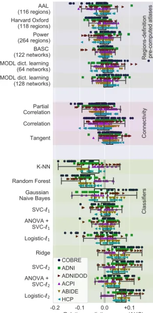
-0.2 -0.1 0.0 +0.1 Relative prediction scores (AUC) AAL (116 regions) Harvard Oxford (118 regions) Power (264 regions) BASC (122 networks) MODL dict. learning (64 networks) MODL dict. learning (128 networks) Partial Correlation Correlation Tangent K-NN Random Forest Gaussian Naive Bayes SVC-1 ANOVA + SVC-1 Logistic-1 Ridge SVC-2 ANOVA + SVC-2 Logistic-2
Regions-definition pre-computed atlases
Connectivity Classifiers COBRE ADNI ADNIDOD ACPI ABIDE HCP
Figure 7: Pipelining choices with precomputed regions, across six datasets: Marginal distribution of relative prediction scores, using only pre-computed atlases for regions definition, where MODL is a parcellation built using a form of Online dictionary learn-ing. Restricting to pre-computed regions and adding a different dataset (HCP) gives results consistent withFigure 5,4, and3: best choices are regions defined functionally, with decomposition meth-ods (MODL) followed by clustering methmeth-ods (BASC), tangent-space parametrization of connectivity, and `2-regularized logistic
regres-sion. The box displays the median and quartiles, while the whiskers give the 5thand 95thpercentiles. Table A1reports the correspond-ing absolute scores.
5. Discussion
An increasing amount of studies use predictive mod-els on functional connectomes, for instance in population-imaging settings to relate brain activity to psychological traits or to build biomarkers of pathologies. While the basic steps of a pipeline are fairly universal –definition of brain regions, construction of an interaction matrix, and
supervised learning– studies in the literature show many methodological variants (Table A2). Recommendations on methods that perform well can increase practitioner’s pro-ductivity and limit vibration effects that risk undermin-ing the reliability of biomarkers (Varoquaux, 2017). A challenge to such recommendations is the heterogeneity of prediction settings, for instance across different acquisition centers or clinical questions.
Here, we investigate methodological choices across 6 databases covering different clinical questions and behav-ioral task. We systematically compare commonly used functional connectome-based prediction methods. We find that some trends emerge, despite a large variance due to variability across subjects –visible across the folds– and across cohorts and clinical questions. Non-sparse linear models, such as logistic regression, appear as a good de-fault choice of classifier. The lack of success of sparse approaches suggests that the discriminant signal is dis-tributed across the functional connectome for the tasks we study. The tangent-space parametrization of func-tional connectomes brings improvements to prediction ac-curacy. With regards to nodes of the functional connec-tomes, defining them from rest-fMRI data gives slight ben-efits in prediction. Linear decomposition methods, such as dictionary learning or ICA, are good approaches to define these nodes from the rest-fMRI data at hand. Unlike clus-tering methods base on “hard” assignment, they provide a soft assignment to regions, enabling to capture a form of uncertainty in the definition of regions. Alternatively, the MODL15 (Mensch et al., 2016a) or BASC (Bellec
et al., 2010) atlases provide good readily-available nodes that simplify the process and alleviate computational cost. The good analytic performance of pre-computed atlases is promising and calls for further study. Establishing stan-dard atlases brings significant computational benefits, as the definition of regions and the extraction of signal is the most computation-intensive part of the pipeline –in partic-ular when performed inside a nested cross-validation loop. We found that using around 100 networks (corresponding to 150 regions) was sufficient for good prediction, though for many region-definition approaches a finer resolution did not hurt average prediction accuracy but only increased variance.
Overall, these results are consistent with the practice of the field. Preliminary comparisons in Abraham et al. (2017) on a single cohort revealed similar trends though ICA had performed poorly while here, with more system-atic benchmarking, it appears to be a good solution. ICA has been used to define functional parcellations or nodes of functional connectomes by many groups (Kiviniemi et al., 2009;Rashid et al.,2014;Smith et al., 2015; Miller et al., 2016). More generally, it is well recognized that the nodes should be defined to match functional networks (Smith et al., 2011). Logistic regression, or the closely-related
15
https://team.inria.fr/parietal/files/2018/10/MODL_rois. zip
SVM, is the go-to classifier for many. Tangent-space parametrization of the connectivity matrix is more exotic, probably due to the mathematical complexity of its origi-nal presentation. However, it is gaining traction outside of methods studies (Colclough et al., 2017; Ng et al., 2017) and is simple to implement, as summarized in Appendix A.
To enable comparison across different cohorts, we fo-cused on 2-class classification problems. However, the results in terms of regions definition and connectivity parametrization should extend to other supervised learn-ing settlearn-ings, such as regression –e.g. for age prediction (Liem et al., 2017)– multi-output approaches as with Canonical Correlation Analysis popular in large-scale pop-ulation imaging settings (Smith et al.,2015;Miller et al., 2016) for dimensional approaches to psychology.
Limitations and Challenges. The main limitation of our study is probably that we had to make choices and focus on the most popular methods. Indeed, to study system-atically methods avoiding overfit requires computational-intense nested cross-validation (where the nesting is re-quired to set the methods’ internal parameters). In par-ticular, we did not investigate Total-Variation constrained dictionary learning (TV-MSDL, Abraham et al. (2013)). This approach defines regions by imposing spatial struc-ture in a linear-decomposition model. In a previous study, we found it promising (Abraham et al., 2017), but it en-tailed too large of a computational cost for this multi-cohort study. Another important class of methods that this study did not investigate are biomarkers based on graph-theoretical approaches. Indeed, we benchmarked variants of a specific pipeline –region definition, followed by construction of a connectivity matrix, and supervised learning on it. Graph-theoretical approaches are an ad-ditional step to add to this pipeline. A full study of all options with this additional step would result in a com-binatorial explosion of pipelines and prohibitive computa-tional costs. We hope that the good choices of regions for edge-level models outlined in this study is also a good one for graph-theoretical approaches and that further studies can focus on exploring only a subset of the options covered here.
With evolving techniques, characteristics of data change, and optimal choices may evolve. However, the consistency of results on HCP suggest that our conclu-sions apply to high-quality datasets using state of the art techniques. A potential concern is the low accuracy for markers of drug abuse in subjects from ACPI datasets, possibly because the number of subjects is small or because ADHD status confounds drug-abuse predictions even af-ter regressing it out. Nevertheless, our pipelines achieved similar accuracy as reported in a previous study on the same data (Meszl´enyi et al., 2016). Finally, the analysis performed here can only outline trends across datasets. Indeed, the study does not establish that a pipeline choice strictly dominates others (see notes on statistical analysis
Step Recommendation
1: region extraction Functional regions,
eg Dictionary learning or ICA 2: connectivity matrix Tangent-space embedding 3: supervised learning Non-sparse linear model,
eg logistic regression or SVM
Table 3: Recommendations for rest-fMRI based prediction pipeline.
in Appendix J), but it gives expected improvements. In term of expected improvement, the choice of classifier is the most important, as going from a poor to a good choice can improve the AUC by more than .1. Both choice of re-gion and choice of parametrization bring smaller expected improvements.
6. Conclusion
Predictive models on rest-fMRI bring the promise of robust and reliable biomarkers: given new brain imaging data, they should give accurate predictions of clinics or behavior (Woo et al., 2017). The framework of the func-tional connectomes grounds well the analysis of rest-fMRI; yet instantiating it still calls for many arbitrary choices.
Our study reveals trends that can provide good de-faults to practitioners, summarized on Table 3: regions defined from functional data, for instance with ICA or dictionary learning as in the pre-computed MODL atlas, representing connectivity with the tangent embedding of covariance matrices, and using a non-sparse linear model, such as a logistic regression. In particular, good defaults can limit the combinatorial explosion of analytic pipelines, which decreases the computational cost of running a study and makes its conclusion more robust statistically. Yet, as it is well known in machine learning (Wolpert, 1996), there cannot be a one-size-fits-all solution to data analysis: optimal choices will differ on datasets with very different properties from the datasets studied here.
Acknowledgments
This work is funded by NiConnect project (ANR-11-BINF-0004 NiConnect) and the CATI project. We also thank to the open-source data community and pre-processed data initiatives for giving access to rest-fMRI datasets. Data collection and sharing for this project was funded by the Alzheimer’s Disease Neuroimaging Initiative (ADNI) (National Institutes of Health Grant U01 AG024904) and DOD ADNI (Department of Defense award number W81XWH-12-2-0012). ADNI is funded by the National Institute on Aging, the National In-stitute of Biomedical Imaging and Bioengineering, and through generous contributions from the following: Ab-bVie, Alzheimer’s Association; Alzheimer’s Drug Discov-ery Foundation; Araclon Biotech; BioClinica, Inc.; Biogen;
Bristol-Myers Squibb Company; CereSpir, Inc.; Cogstate; Eisai Inc.; Elan Pharmaceuticals, Inc.; Eli Lilly and Com-pany; EuroImmun; F. Hoffmann-La Roche Ltd and its af-filiated company Genentech, Inc.; Fujirebio; GE Health-care; IXICO Ltd.; Janssen Alzheimer Immunotherapy Re-search and Development, LLC.; Johnson and Johnson Pharmaceutical Research and Development LLC.; Lumos-ity; Lundbeck; Merck and Co., Inc.; Meso Scale Diagnos-tics, LLC.; NeuroRx Research; Neurotrack Technologies; Novartis Pharmaceuticals Corporation; Pfizer Inc.; Pira-mal Imaging; Servier; Takeda Pharmaceutical Company; and Transition Therapeutics. The Canadian Institutes of Health Research is providing funds to support ADNI clin-ical sites in Canada. Private sector contributions are fa-cilitated by the Foundation for the National Institutes of Health (www.fnih.org). The grantee organization is the Northern California Institute for Research and Education, and the study is coordinated by the Alzheimer’s Therapeu-tic Research Institute at the University of Southern Cali-fornia. ADNI data are disseminated by the Laboratory for Neuro Imaging at the University of Southern California. Ethics statement
No experiments on living beings were performed for this study. Hence IRB approval was not necessary. The data that we used were acquired in original studies that had received approval by the original institution’s IRB. All data were used accordingly to respective usage guidelines. Data and code availability
The original data can be retrieved from: • COBREhttp://cobre.mrn.org/
• ADNI & ADNIDOD www.adni-info.org
• ACPI http://fcon_1000.projects.nitrc.org/indi/ ACPI/html/ • ABIDEhttp://preprocessed-connectomes-project. org/abide/index.html • HCP https://www.humanconnectome. org/study/hcp-young-adult/document/ 900-subjects-data-release
Code to reproduce the experiments can be re-trieved from: https://github.com/KamalakerDadi/ benchmark_rsfMRI_prediction
To facilitate reproduction, we also share time series, though without labels to comply with origi-nal data usage conditions, on https://github.com/ KamalakerDadi/benchmark_rsfMRI_prediction/blob/ master/downloader.py
7. References
Abraham, A., Dohmatob, E., Thirion, B., Samaras, D., Varoquaux, G., 2013. Extracting brain regions from rest fMRI with total-variation constrained dictionary learning, in: MICCAI, p. 607.
Abraham, A., Dohmatob, E., Thirion, B., Samaras, D., Varoquaux, G., 2014a. Region segmentation for sparse decompositions: better brain parcellations from rest fMRI. Frontiers in neuroinformatics 8.
Abraham, A., Milham, M.P., Di Martino, A., Craddock, R.C., Sama-ras, D., Thirion, B., Varoquaux, G., 2017. Deriving reproducible biomarkers from multi-site resting-state data: An autism-based example. NeuroImage 147, 736–745.
Abraham, A., Pedregosa, F., Eickenberg, M., Gervais, P., Mueller, A., Kossaifi, J., Gramfort, A., Thirion, B., Varoquaux, G., 2014b. Machine learning for neuroimaging with scikit-learn. Frontiers in neuroinformatics 8.
Anderson, A., Douglas, P.K., Kerr, W.T., Haynes, V.S., Yuille, A.L., Xie, J., Wu, Y.N., Brown, J.A., Cohen, M.S., 2014. Non-negative matrix factorization of multimodal MRI, fMRI and phenotypic data reveals differential changes in default mode subnetworks in ADHD. NeuroImage 102, 207–219.
Arbabshirani, M.R., Kiehl, K.A., Pearlson, G.D., Calhoun, V.D., 2013. Classification of schizophrenia patients based on resting-state functional network connectivity. Frontiers in Neuroscience 7.
Arbabshirani, M.R., Plis, S., Sui, J., Calhoun, V.D., 2017. Single subject prediction of brain disorders in neuroimaging: Promises and pitfalls. NeuroImage 145, 137–165.
Barachant, A., Bonnet, S., Congedo, M., Jutten, C., 2013. Classifi-cation of covariance matrices using a riemannian-based kernel for bci applications. Neurocomputing 112, 172 – 178.
Bassett, D.S., Nelson, B.G., Mueller, B.A., Camchong, J., Lim, K.O., 2012. Altered resting state complexity in schizophrenia. NeuroIm-age 59, 2196–2207.
Beckmann, C.F., Smith, S.M., 2004. Probabilistic independent com-ponent analysis for functional magnetic resonance imaging. Trans Med Im 23, 137.
Behzadi, Y., Restom, K., Liau, J., Liu, T., 2007. A component based noise correction method (compcor) for BOLD and perfusion based fMRI. Neuroimage 37, 90.
Bellec, P., Rosa-Neto, P., Lyttelton, O., Benali, H., Evans, A., 2010. Multi-level bootstrap analysis of stable clusters in resting-state fMRI. NeuroImage 51, 1126.
Biswal, B., Mennes, M., Zuo, X., Gohel, S., Kelly, C., Smith, S., Beckmann, C., et al., 2010. Toward discovery science of human brain function. Proc Ntl Acad Sci 107, 4734.
Breiman, L., 2001. Random forests. Machine Learning 45, 5. Brier, M.R., Mitra, A., McCarthy, J.E., Ances, B.M., Snyder, A.Z.,
2015. Partial covariance based functional connectivity computa-tion using ledoit–wolf covariance regularizacomputa-tion. NeuroImage 121, 29–38.
Brown, C.J., Hamarneh, G., 2016. Machine learning on human con-nectome data from mri. arXiv:1611.08699 .
Calhoun, V., Sui, J., Kiehl, K., Turner, J., Allen, E., Pearlson, G., 2012. Exploring the psychosis functional connectome: Aberrant intrinsic networks in schizophrenia and bipolar disorder. Frontiers in Psychiatry .
Calhoun, V.D., Adali, T., Pearlson, G.D., Pekar, J.J., 2001. A method for making group inferences from fMRI data using in-dependent component analysis. Hum Brain Mapp 14, 140. Carp, J., 2012. On the plurality of (methodological) worlds:
Esti-mating the analytic flexibility of fMRI experiments. Frontiers in neuroscience 6.
Chen, G., Ward, B.D., Xie, C., Li, W., Wu, Z., Jones, J.L., Franczak, M., Antuono, P., Li, S.J., 2011. Classification of alzheimer dis-ease, mild cognitive impairment, and normal cognitive status with large-scale network analysis based on resting-state functional MR imaging. Radiology 259, 213–221.
Cheng, W., Ji, X., Zhang, J., Feng, J., 2012. Individual classification of ADHD patients by integrating multiscale neuroimaging markers and advanced pattern recognition techniques. Frontiers in Systems Neuroscience 6.
Colclough, G.L., Smith, S.M., Nichols, T.E., Winkler, A.M., Sotiropoulos, S.N., Glasser, M.F., Van Essen, D.C., Woolrich, M.W., 2017. The heritability of multi-modal connectivity in hu-man brain activity. eLife 6, e20178.
Cover, T., Hart, P., 1967. Nearest neighbor pattern classification. IEEE Trans. Inf. Theor. 13, 21–27.
Craddock, C., Benhajali, Y., Chu, C., Chouinard, F., Evans, A., Jakab, A., Khundrakpam, B.S., Lewis, J.D., Li, Q., Milham, M., Yan, C., Bellec, P., 2013. The neuro bureau preprocessing initia-tive: open sharing of preprocessed neuroimaging data and deriva-tives ¡br /¿. Frontiers in Neuroinformatics .
Craddock, C., Sikka, S., Cheung, B., Khanuja, R., Ghosh, S.S., Yan, C., Li, Q., Lurie, D., Vogelstein, J., Burns, R., Colcombe, S., Mennes, M., Kelly, C., Di Martino, A., Castellanos, F.X., Milham, M., . Towards automated analysis of connectomes: The config-urable pipeline for the analysis of connectomes (c-pac). Frontiers in Neuroinformatics .
Craddock, R.C., Holtzheimer, P.E., Hu, X.P., Mayberg, H.S., 2009. Disease state prediction from resting state functional connectivity. Magnetic Resonance in Medicine 62, 1619.
Craddock, R.C., James, G.A., Holtzheimer, P.E., Hu, X.P., Mayberg, H.S., 2012. A whole brain fMRI atlas generated via spatially constrained spectral clustering. Human brain mapping 33, 1914. Craddock, R.C., Tungaraza, R.L., Milham, M.P., 2015.
Connec-tomics and new approaches for analyzing human brain functional connectivity. GigaScience 4, 13.
Desikan, R., S., S´egonne, F., Fischl, B., Quinn, B., T., Dickerson, B., C., Blacker, D., Buckner, R., L., Dale, A., M., Maguire, R., P., Hyman, B., T., Albert, M., S., Killiany, R., J., 2006. An auto-mated labeling system for subdividing the human cerebral cortex on mri scans into gyral based regions of interest. Neuroimage 31, 968.
Di Martino, A., Yan, C.G., Li, Q., Denio, E., Castellanos, F.X., Alaerts, K., Anderson, J.S., Assaf, M., Bookheimer, S.Y., Dapretto, M., et al., 2014. The autism brain imaging data ex-change: towards a large-scale evaluation of the intrinsic brain ar-chitecture in autism. Molecular psychiatry 19, 659–667.
Dodero, L., Minh, H.Q., Biagio, M.S., Murino, V., Sona, D., 2015. Kernel-based classification for brain connectivity graphs on the riemannian manifold of positive definite matrices, in: Interna-tional Symposium on Biomedical Imaging (ISBI), IEEE. Dosenbach, N.U.F., Nardos, B., Cohen, A.L., Fair, D.A., Power,
J.D., Church, J.A., Nelson, S.M., Wig, G.S., Vogel, A.C., Lessov-Schlaggar, C.N., Barnes, K.A., Dubis, J.W., Feczko, E., Coalson, R.S., Pruett, J.R., Barch, D.M., Petersen, S.E., Schlaggar, B.L., 2010. Prediction of individual brain maturity using fMRI. Science 329, 1358–1361.
Drysdale, A.T., Grosenick, L., et al., 2016. Resting-state connectiv-ity biomarkers define neurophysiological subtypes of depression. Nature Medicine .
Dubois, J., Adolphs, R., 2016. Building a science of individual dif-ferences from fmri. Trends in cognitive sciences 20, 425–443. Dubois, J.C., Galdi, P., Paul, L.K., Adolphs, R., 2018. A distributed
brain network predicts general intelligence from resting-state hu-man neuroimaging data. bioRxiv , 257865.
Elliott, P., Peakman, T.C., et al., 2008. The UK biobank sample handling and storage protocol for the collection, processing and archiving of human blood and urine. International Journal of Epidemiology 37, 234–244.
Fei, F., Jie, B., Zhang, D., 2014. Frequent and discriminative subnet-work mining for mild cognitive impairment classification. Brain Connectivity 4, 347–360.
Fletcher, P., Joshi, S., 2007. Riemannian geometry for the statistical analysis of diffusion tensor data. Signal Processing 87, 250. Fox, M.D., Zhang, D., Snyder, A.Z., Raichle, M.E., 2009. The global
signal and observed anticorrelated resting state brain networks. Journal of neurophysiology 101, 3270–3283.
Friedman, J., Hastie, T., Tibshirani, R., 2008. Sparse inverse covari-ance estimation with the graphical lasso. Biostatistics 9, 432. Gellerup, D., 2016. Discriminating Parkinsons Disease Using
Func-tional Connectivity and Brain Network Analysis. Ph.D. thesis. University of Texas - Arlington.
Gorgolewski, K., Burns, C.D., Madison, C., Clark, D., Halchenko, Y.O., Waskom, M.L., Ghosh, S.S., 2011. Nipype: a flexible, lightweight and extensible neuroimaging data processing frame-work in python. Front Neuroinform 5, 13.
Greicius, M., 2008. Resting-state functional connectivity in neu-ropsychiatric disorders. Current opinion in neurology 21, 424. Guo, H., Cao, X., Liu, Z., Li, H., Chen, J., Zhang, K., 2012.
Ma-chine learning classifier using abnormal brain network topological metrics in major depressive disorder. NeuroReport 23, 1006–1011. Hallquist, M.N., Hillary, F.G., 2018. Graph theory approaches to functional network organization in brain disorders: A critique for a brave new small-world. bioRxiv , 243741.
Hastie, T., Tibshirani, R., Friedman, J., 2009. The elements of sta-tistical learning. Springer.
Hunter, J.D., 2007. Matplotlib: A 2d graphics environment. Com-puting In Science & Engineering 9, 90–95.
Iidaka, T., 2015. Resting state functional magnetic resonance imag-ing and neural network classified autism and control. Cortex 63, 55–67.
Jie, B., Shen, D., Zhang, D., 2014. Brain connectivity hyper-network for MCI classification, in: Medical Image Computing and Computer-Assisted Intervention – MICCAI 2014. Springer Inter-national Publishing, pp. 724–732.
Kahnt, T., Chang, L.J., Park, S.Q., Heinzle, J., Haynes, J.D., 2012. Connectivity-based parcellation of the human orbitofrontal cortex. Journal of Neuroscience , 6240–6250.
Khazaee, A., Ebrahimzadeh, A., Babajani-Feremi, A., 2015. Iden-tifying patients with alzheimer’s disease using resting-state fMRI and graph theory. Clinical Neurophysiology 126, 2132–2141. Kiviniemi, V., Starck, T., Remes, J., Long, X., Nikkinen, J., Haapea,
M., Veijola, J., et al., 2009. Functional segmentation of the brain cortex using high model order group PICA. Hum Brain Map 30, 3865.
Ledoit, O., Wolf, M., 2004. A well-conditioned estimator for large-dimensional covariance matrices. J. Multivar. Anal. 88, 365. Liem, F., Varoquaux, G., Kynast, J., Beyer, F., Masouleh, S.K.,
Huntenburg, J.M., Lampe, L., Rahim, M., Abraham, A., Crad-dock, R.C., et al., 2017. Predicting brain-age from multimodal imaging data captures cognitive impairment. NeuroImage 148, 179–188.
Mazumder, R., Hastie, T., 2012. The graphical lasso: New insights and alternatives. Electronic journal of statistics 6, 2125. Mensch, A., Mairal, J., Thirion, B., Varoquaux, G., 2016a.
Dictio-nary Learning for Massive Matrix Factorization, in: International Conference on Machine Learning, pp. 1737–1746.
Mensch, A., Mairal, J., Thirion, B., Varoquaux, G., 2018. Stochastic subsampling for factorizing huge matrices. IEEE Transactions on Signal Processing 66, 113–128.
Mensch, A., Varoquaux, G., Thirion, B., 2016b. Compressed Online Dictionary Learning for Fast Resting-State fMRI Decomposition, in: Proc. ISBI, p. 1282.
Meszl´enyi, R., Peska, L., G´al, V., Vidny´anszky, Z., Buza, K., 2016. A model for classification based on the functional connectivity pattern dynamics of the brain, in: 2016 Third European Network Intelligence Conference (ENIC), pp. 203–208.
Michel, V., Gramfort, A., Varoquaux, G., Eger, E., Keribin, C., Thirion, B., 2012. A supervised clustering approach for fMRI-based inference of brain states. Pattern Recognition 45, 2041. Milazzo, A.C., Ng, B., Jiang, H., Shirer, W., Varoquaux, G., Poline,
J.B., Thirion, B., Greicius, M.D., 2014. Identification of mood-relevant brain connections using a continuous, subject-driven ru-mination paradigm. Cereb. Cortex 26, 933–942.
Miller, K.L., Alfaro-Almagro, F., et al., 2016. Multimodal popula-tion brain imaging in the UK biobank prospective epidemiological study. Nature Neuroscience .
Mueller, S., Weiner, M., Thal, L., Petersen, R., Jack, C., Jagust, W., Trojanowski, J.Q., Toga, A.W., Beckett, L., 2005. The alzheimers disease neuroimaging initiative. Neuroimaging Clinics of North America 15, 869.
Murphy, K., Birn, R.M., Handwerker, D.A., Jones, T.B., Bandettini, P.A., 2009. The impact of global signal regression on resting state correlations: are anti-correlated networks introduced? Neuroim-age 44, 893–905.
Ng, B., Dressler, M., Varoquaux, G., Poline, J.B., Greicius, M., Thirion, B., 2014. Transport on Riemannian Manifold for Func-tional Connectivity-based Classification, in: MICCAI - 17th Inter-national Conference on Medical Image Computing and Computer Assisted Intervention.
Ng, B., Varoquaux, G., Poline, J.B., Thirion, B., Greicius, M.D., Poston, K.L., 2017. Distinct alterations in parkinson’s medication-state and disease-medication-state connectivity. NeuroImage: Clinical 16, 575–585.
Nielsen, J.A., Zielinski, B.A., Fletcher, P.T., Alexander, A.L., Lange, N., Bigler, E.D., Lainhart, J.E., Anderson, J.S., 2013. Multisite functional connectivity MRI classification of autism: ABIDE re-sults. Frontiers in Human Neuroscience 7.
Pedregosa, F., Varoquaux, G., Gramfort, A., et al., 2011. Scikit-learn: Machine learning in Python. Journal of Machine Learning Research 12, 2825.
Pennec, X., Fillard, P., Ayache, N., 2006. A Riemannian framework for tensor computing. Int J Comp Vision 66, 41.
Perrot, M., Riviere, D., Tucholka, A., Mangin, J.F., 2009. Joint Bayesian Cortical Sulci Recognition and Spatial Normalization, in: IPMI.
Power, J., Cohen, A., Nelson, S., Wig, G., Barnes, K., Church, J., Vogel, A., Laumann, T., Miezin, F., Schlaggar, B., Petersen, S., 2011. Functional network organization of the human brain. Neu-ron 72, 665–678.
Power, J.D., Barnes, K.A., Snyder, A.Z., Schlaggar, B.L., Petersen, S.E., 2012. Spurious but systematic correlations in functional con-nectivity mri networks arise from subject motion. Neuroimage 59, 2142–2154.
Pruett, J.R., Kandala, S., Hoertel, S., Snyder, A.Z., Elison, J.T., Nishino, T., Feczko, E., Dosenbach, N.U., Nardos, B., Power, J.D., Adeyemo, B., Botteron, K.N., McKinstry, R.C., Evans, A.C., Ha-zlett, H.C., Dager, S.R., Paterson, S., Schultz, R.T., Collins, D.L., Fonov, V.S., Styner, M., Gerig, G., Das, S., Kostopoulos, P., Con-stantino, J.N., Estes, A.M., Petersen, S.E., Schlaggar, B.L., Piven, J., 2015. Accurate age classification of 6 and 12 month-old infants based on resting-state functional connectivity magnetic resonance imaging data. Developmental Cognitive Neuroscience 12, 123–133. Qiu, A., Lee, A., Tan, M., Chung, M.K., 2015. Manifold learning on brain functional networks in aging. Medical Image Analysis 20, 52 – 60.
Rahim, M., Thirion, B., Varoquaux, G., 2017. Population-shrinkage of covariance to estimate better brain functional connectivity, in: International Conference on Medical Image Computing and Computer-Assisted Intervention, Springer. pp. 460–468.
Rashid, B., Arbabshirani, M.R., Damaraju, E., Cetin, M.S., Miller, R., Pearlson, G.D., Calhoun, V.D., 2016. Classification of schizophrenia and bipolar patients using static and dynamic resting-state fMRI brain connectivity. NeuroImage 134, 645–657. Rashid, B., Damaraju, E., Pearlson, G.D., Calhoun, V.D., 2014. Dynamic connectivity states estimated from resting fMRI iden-tify differences among schizophrenia, bipolar disorder, and healthy control subjects. Frontiers in human neuroscience 8, 897. Richiardi, J., Eryilmaz, H., Schwartz, S., Vuilleumier, P., Van
De Ville, D., 2010. Decoding brain states from fMRI connectivity graphs. NeuroImage .
Rosa, M.J., Portugal, L., Hahn, T., Fallgatter, A.J., Garrido, M.I., Shawe-Taylor, J., Mourao-Miranda, J., 2015. Sparse network-based models for patient classification using fMRI. NeuroImage 105.
Rubinov, M., Sporns, O., 2011. Weight-conserving characterization of complex functional brain networks. NeuroImage 56, 2068. Shen, H., Wang, L., Liu, Y., Hu, D., 2010. Discriminative analysis
of resting-state functional connectivity patterns of schizophrenia using low dimensional embedding of fMRI. NeuroImage 49, 3110. Shirer, W., Ryali, S., Rykhlevskaia, E., Menon, V., Greicius, M., 2012. Decoding subject-driven cognitive states with whole-brain connectivity patterns. Cerebral Cortex 22, 158.
Simmons, J.P., Nelson, L.D., Simonsohn, U., 2011. False-positive psychology: Undisclosed flexibility in data collection and analysis allows presenting anything as significant. Psychological science 22, 1359.
Smith, S., Miller, K., Salimi-Khorshidi, G., Webster, M., Beckmann, C., Nichols, T., Ramsey, J., Woolrich, M., 2011. Network mod-elling methods for fMRI. Neuroimage 54, 875.
Smith, S.M., Nichols, T.E., Vidaurre, D., Winkler, A.M., Behrens, T.E., Glasser, M.F., Ugurbil, K., Barch, D.M., Van Essen, D.C., Miller, K.L., 2015. A positive-negative mode of population covari-ation links brain connectivity, demographics and behavior. Nature neuroscience 18, 1565–1567.
Sporns, O., Tononi, G., Kotter, R., 2005. The human connectome: a structural description of the human brain. PLoS Comput Biol 1, e42.
Thirion, B., Varoquaux, G., Dohmatob, E., Poline, J., 2014. Which fMRI clustering gives good brain parcellations? Name: Frontiers in Neuroscience 8, 167.
Tzourio-Mazoyer, N., Landeau, B., Papathanassiou, D., Crivello, F., Etard, O., Delcroix, N., Mazoyer, B., Joliot, M., 2002. Automated anatomical labeling of activations in SPM using a macroscopic anatomical parcellation of the MNI MRI single-subject brain. Neuroimage 15, 273.
Van Essen, D., Ugurbil, K., Auerbach, E., Barch, D., Behrens, T., Bucholz, R., Chang, A., Chen, L., Corbetta, M., Curtiss, S., Della Penna, S., Feinberg, D., Glasser, M., Harel, N., Heath, A., Larson-Prior, L., Marcus, D., Michalareas, G., Moeller, S., Oostenveld, R., Petersen, S., Prior, F., Schlaggar, B., Smith, S., Snyder, A., Xu, J., Yacoub, E., 2012. The human connectome project: A data acquisition perspective. NeuroImage 62, 2222–2231.
Van Essen, D.C., Smith, et al., 2013. The wu-minn human connec-tome project: an overview. Neuroimage 80, 62–79.
Vanderweyen, D., , Munsell, B.C., Mintzer, J.E., Mintzer, O., Ga-jadhar, A., Zhu, X., Wu, G., Joseph, J., 2015. Identifying abnor-mal network alterations common to traumatic brain injury and alzheimer’s disease patients using functional connectome data, in: Machine Learning in Medical Imaging. Springer International Publishing, pp. 229–237.