Identifying and Explaining the Number of Regimes Driving Asset Returns

(1)

HAL Id: halshs-00658544

https://halshs.archives-ouvertes.fr/halshs-00658544

Submitted on 10 Jan 2012

HAL is a multi-disciplinary open access

archive for the deposit and dissemination of

sci-entific research documents, whether they are

pub-lished or not. The documents may come from

teaching and research institutions in France or

abroad, or from public or private research centers.

L’archive ouverte pluridisciplinaire HAL, est

destinée au dépôt et à la diffusion de documents

scientifiques de niveau recherche, publiés ou non,

émanant des établissements d’enseignement et de

recherche français ou étrangers, des laboratoires

publics ou privés.

Driving Asset Returns

Mathieu Gatumel, Florian Ielpo

To cite this version:

Mathieu Gatumel, Florian Ielpo. Identifying and Explaining the Number of Regimes Driving Asset

Returns. 2011. �halshs-00658544�

(2)

Identifying and Explaining the Number of Regimes

Driving Asset Returns

Mathieu Gatumel

Florian Ielpo

CAHIER DE RECHERCHE n°2011-06 E2

Unité Mixte de Recherche CNRS / Université Pierre Mendès France Grenoble 2 150 rue de la Chimie – BP 47 – 38040 GRENOBLE cedex 9

(3)

Driving Asset Returns

Mathieu

Gatumel

∗ University of Grenoble

Florian

Florian Ielpo

Ielpo

†

Lombard Odier Investment Managers Paris 1 University

April 8, 2011

Abstract Abstract Abstract Abstract

A shared belief in the financial industry is that markets are driven by two types of regimes. Bull markets would be characterized by high returns and low volatility whereas bear markets would display low returns coupled with high volatility. Modelling the dynamics of different asset classes (stocks, bonds, commodities and currencies) with a Markov-Switching model and using a density-based test, we re- ject the hypothesis that two regimes are enough to capture asset returns’ evolutions. Once the accuracy of our test methodology has been assessed through Monte Carlo experiments, our empirical results point out that between three and five regimes are required to capture the features of each asset’s distribution. A probit multinomial regression highlights that only a part of the underlying number of regimes is par- tially explained by the absolute average yearly risk premium and by distributional charateristics of the returns such as the kurtosis.

∗ _{Corresponding author. University of Grenoble, IUT2-CERAG, Place Doyen Gosse, 38031}

Grenoble, France. Email: mathieu.gatumel@iut2.upmf-grenoble.fr. Tel.: +33.4.76.28.45.78.

† _{Lombard Odier Asset Management, rue de la Corraterie 11, 1204 Geneva, Switzerland and}

University Paris 1 Panthéon - CERMSEM, Maison des Sciences Economiques, 106 Boulevard de l’Hopital, 75013 Paris, France. Email: florian.ielpo@ensae.org.

(4)

1

1 1 Introduction

Introduction

Financial asset prices fluctuate in a tick-by-tick fashion to a globalized news flow. The nature and frequency of this flow has a tremendous impact on the dynamics of financial markets, as reflected by the evolutions of the major indices usually used by financial data providers and newspaper to summarize the flavor of the financial week. In this summarizing process, two kinds of episodes are usually identified and used as labels: a growing valuation of risky assets in a low volatility environment is referred to as “bull market”. On the contrary, “bear market” is the wording used to describe a period during which government bonds are used as safe havens whereas risky assets deliver strongly negative returns and volatility goes through a sharp increase. Useful though these approximations may be, this article questions the existence of these two regimes in financial markets. Given the complexity and deep- ness of the information reflected in asset prices, there are great chances that there are more than just bulls and bears in financial markets.

Simplifications are commonplace when facing complex mechanism: this bull/bear distinction nourished a large financial literature - part of which is academic. A selection of these academic articles turned to Hamilton (1989)’s Markov Switching model as with such a model, bull and bear days can be measured through probabilities. This combination led to strong improvements in our understanding of the behavior of financial markets: see for example what is presented in Chauvet and Potter (2000) or Ang and Bekaert (2002a,2002b). Beyond the insight regarding the times series dynamics of returns, this approach still suffers from one drawback: the number of market regimes is assumed before the estimation and this hypothesis was hardly checked in the literature. However and more recently Maheu et al. (2010) describe how expanding the assumed number of regimes - adding bullish bear and bearish bull regimes to the sole bull/bear usual assumption - is essential to portfolio managers.

This article intends to fill a gap: we present a test to determine the number of regimes implicit in returns based on a conditional density argument when the underlying model is a standard Markov Switching model with n regimes. This test is inspired by the likelihood ratio tests for possibly non nested models presented in Vuong (1989) and Amisano and Giacomini (2007). A Monte Carlo test shows that our approach allows us to consistently estimate the number of regimes. We turn our attention to a large dataset of weekly returns on several indices: we show that only two foreign exchange rates - namely the Swiss Franc and the Yen versus Dollar - can be modeled by a two-regime MS model. For most of the assets covered here, the number of regimes is equal to three. This additional regime is of various natures and asset dependent. For selected cases, the number of regimes can be equal up to 6, as it is the case for the European High Yield index. We discuss the persistence and performances under each regime, underlining that the bull/bear specification may be oversimplifying a complex reality. Finally, we show that the number of states estimated has only a weak link with the distributional properties of returns.

This article is structured as follows: Section 2 presents the underlying modeling methodology, jointly with the Monte Carlo evaluation of the test used to estimate the number of regimes. Section 3 discusses the elements involved in our dataset. Section 4 presents a detailed discussion of the results. Section 5 concludes.

(5)

2

2 2 T

T

Testing

esting

esting for

for

for the

for

the

the number

the

number of

number

of

of regimes

regimes

regimes implied

implied by

implied

by

by fi

fi

fi----

nancial

nancial returns’

returns’

returns’ dynamics

returns’

dynamics

This section is devoted to the presentation of the material needed for the test used in this article. We first briefly review the basics of Hamilton (1989)’s switching model before turning to the presentation of specification test inspired by Vuong (1989) and Amisano and Giacomini (2007).

2.1

2.1 2.1 A

A

A brief

brief

brief presentation

presentation

presentation of

presentation

of the

of

the

the Markov

Markov

Markov Switching

Switching

Switching model

Switching

model

We provide the reader with a short presentation of Hamilton (1989)’s markov switching model. This model has initially been introduced in the literature by focusing on the US business cycle. Its use to estimate the regimes in financial markets has been since developped in various articles such as Chauvet and Potter (2000), Ang and Bekaert (2002a,2002b) or more recently Maheu et a. (2010). This time series model aims at modelling and estimating the changes in regimes that affect economic and market series. It relies on the assumption that the probability to move from one state to the other is time varying, while the transition probabilities are constant. We present the basic intuitions using a two-regimes MS model before turning to a general case. Let rt be the logarithmic return on a given asset at time t, for the

holding period between t − 1 and t. Let st be an integer value variable that is equal

to 1 (respectively 2) at time t if regime 1 (respectively 2) prevails in the economy. Given that the regime i prevails, the conditional distribution of returns is as follows:

rt ∼ N (µi , σi ). (1)

The probability to be in regime 1 at time t writes:

P (st = 1) = P (st = 1|st−1 = 1) × P (st−1 = 1) + P (st = 1|st−1 = 2) × P (st−1 = 2). (2)

P (st = 1|st−1 = 1) is assumed to be constant and equal to p, and P (st = 2|st−1 = 1) =

1 − p. With a similar argument, P (st = 2|st−1 = 2) = q and P (st = 1|st−1 = 2) = 1 − q.

These transition probabilities can be gathered into a transition matrix as follows: p 1 − p , (3) such that Π = 1 − q q Pt = ΠPt−1 , (4) with Pt = (P (st = 1), P (st = 2)) >

. The parameters driving the model are thus the moment associated to asset returns for each state and the matrix Π. The usual estimation strategy is a maximum likelihood one, based on the filtering approach developed in Hamilton (1989).

This two-regime case can be generalised to a n-regime one: in such a case, st can

take integer values ranging from 1 to n, and the Π matrix become a n × n matrix.

2.2

2.2 2.2 T

Testing

T

esting

esting for

esting

for

for the

the

the number

the

number

number of

number

of regimes

of

regimes

regimes in

regimes

in

in a

a

a MS

a

MS

MS model

MS

model

As presented in the introduction, little attention has been devoted in the literature to testing the optimal number of regimes that are actually driving financial returns.

(6)

t

n1 ,n2

The approach that we propose here is inspired by the LR tests presented in Vuong (1989) and Amisano and Giacomini (2007) and aims at comparing two models in terms of goodness of fit of the returns’s distribution.

Let fn1 (rt ; θˆn1 ) be the likelihood function assciated to an estimated Markov-Switching

model with n1 states. Let fn2 (rt ; θˆn2 ) be a similar quantity in the case of a MS model

with n2 regimes. θni is the vector of the parameters to be estimated by maximum

likelihood in the ni -regime case. the two specifications are compared through their

associated log density computed with the estimated sample. Let zn1 ,n2 _{be the follow-}

ing quantity:

z_t = log fn1 (rt ; θˆn1 ) − log fn2 (rt ; θˆn2 ). (5)

The approach proposed here is based on the following test statistics:

1 PT n1 ,n2 tn1 ,n2 = T t=1 z_{√ ,}t (6) σ ˆn1 ,n2 T

where T is the total number of available observations in the sample used to estimate the parameters, and σˆn1 ,n2 a properly selected estimator of the standard deviation of

1 PT n1 ,n2

T t=1 zt . We propose to estimate this standard deviation using a Newey West

(1987) estimator.

Under the null hypothesis that both models provide and equivalent fit of the returns’ distribution, Amisano and Giacomini (2007)’s Theorem 1 provides the asymptotic distribution of this test statistics:

tn1 ,n2 ∼ N (0, 1). (7)

This test statistics allow us to compare non nested and nested models as well. We assume that the conditions stated in the theorem 1 of Amisano and Giacomini are granted in our case.

The main issue with this kind of test is that when comparing the in-sample fit of the distribution, the bigger the number of parameters and the better the fit of the distribution obtained. Hence, by dwelling our analysis on a in-sample test of MS models with a number of regimes ranging between 1 and 10, we are very likely to decide that the model with 10 regimes should be retained for it provides us with the best fit possible. To circumvent this problem, we propose to retain the number of regimes that delivers the best fit from the previous statistics point of view, while being as parsimonious as possible. Hence, our approach combines the previous test inspired by Vuong (1987) and Amisano and Giacomini (2007) to the following number of regime selection procedure:

Step 1: Start with a number of regime equal to 1. Estimate the parameters. Step 2: Estimate the parameters of a two-regime model. Compare the model with two regimes to the model with one regime: if t2,1 > 1.96, go to Step 3. If

not, select the model with 1 regime.

Step 3: Estimate the parameters of a three-regime model. Compare the model with three regimes to the model with two regimes: if t3,2 > 1.96, go to Step 4. If

not, select the model with 2 regimes.

(7)

With this selection procedure, we select the most parsimonious specification for the number of regimes that provides a statistical superior fit to any specification using a lower number of regimes while being equivalent to a model with one more regime. By doing so, we are due to select the number of regimes that does not overfit the returns’ distribution, while providing us with an approximate measure of the structural number of regimes driving the returns.

2.3

2.3 2.3 A

A

A Monte

Monte

Monte Carlo

Carlo

Carlo investigation

investigation of

investigation

of

of our

our

our test

test

test methodology

methodology

Before applying the previous methodology to a real dataset of financial returns, we ran two different Monte Carlo tests. These tests aim at gauging the ability of the test to estimate the number of underlying regimes when this number is known and the model is a Markov Swithching model.

We use the two different specifications: a MS model with three regimes and another one with five regimes, as they are two of the common cases found in the empirical results presented in the next Section. These models present a special interest for our work, as they differ from the usual bull-bear dyptic: the test would behave very badly if it was to diagnose two underlying regimes when there are indeed more. The parameters used in this Monte Carlo exercise are obtained by estimating a MS(3) using the Eurostoxx index’s returns, and the parameters for the MS(5) are obtained from the US High Yield index’s returns. The parameters are the following:

– The 3 regime model is characterized by two types of bear episodes and a single type of bull regime. The moderate and very volatile bear regime is the dom- inant one as 47% of the trading weeks for the Eurostoxx deliver a negative return to the investor. What is more, around 63% of the dataset is made of weekly returns between -2.5% and 2.5% which is a rather average low weekly return for an equity index.

µ1 = − 0.63%, σ1 = 5.69%, (8) µ2 = 1.23%, σ2 = 1.74%, (9) µ3 = − 2.06%, σ3 = 1.82%, (10)  0.93 0.07 0.00  P =  0.00 0.62 0.38  (11) 0.06 0.70 0.25

– The 5 regime model is characterized by four types of bear regimes, involving different various scales of expected returns and their associated volatility. The most persistent regime is regime 1: for this bullish regime, investors holding high yield bonds benefit from a 0.09% (=4.82%/52) weekly return on average. Amongst of the bearish regimes, one should differenciate strongly negative expected returns with medium volatility from moderatly negative returns coming alongside a large volatility. This latter case corresponds to a large uncertainty mixed a progressive widening of risk premia in the high yield market. On a yearly basis, we get:

(8)

µ1 = 4.82%, σ1 = 2.30%, (12) µ2 = − 10.78%, σ2 = 25.04%, (13) µ3 = 50.55%, σ3 = 5.80%, (14) µ4 = − 28.58%, σ4 = 5.82%, (15) µ5 = 21.62%, σ5 = 2.67%, (16)  0.96 0.00 0.00 0.04 0.00   0.00 0.94 0.00 0.06 0.00  P =   _0.06 0.00 0.63 0.00 0.32   (17) 0.00 0.02 0.14 0.80 0.04    0.02 0.00 0.06 0.12 0.80

We believe these two specifications provide two stylized and realistic settings with which we should try to assess the quality of the test presented above.

For each of these specifications we sample 650 weeks of returns, as the samples used in the empirical section are of that length. That is 12 years and a half of returns, which involves in our view enough market episodes to provide us with a rather structural view about the regimes affecting asset returns. For each of the simulated samples, we reestimate the MS(i) parameters, for i ranging from 1 to 10. Once the parameters are estimated, we run the test to select the optimal number of regime. The Table 2 provides descriptive statistics regarding the optimal number of regimes. Given the discrete nature of the support of the number of regimes, we are mostly interested in the median of the selected stats, that is the state that has the highest probability to be selected. Both in the 3- and the 5-regime cases, the median matches the real number of regimes. This is essential to our article. We nonetheless discuss the average number of state: when in the 5-regime case the sample average is also 5, in the 3-regime one, we get a slightly different story. In this case, the average is equal to 3.5, underlying the fact that one average the test seems to over-estimate the number of regimes. The skewness presented in this table corroborate this fact. The frequencies of for each state are presented in Figure 1. The figure presents the frequency for which the state i has been selected out of the 10 000 replications. The test does not seem to have a perfect precision, given the non-zero frequencies at which it selects a number of state different from the true one. This will be something to be kept in mind when investigating the real dataset results. Finally, we find that when the true model is either a MS(3) or a MS(5), the frequency at which a model with 2 regimes is selected is fairly close to zero. Again, this point will be essential in the forthcoming section.

3

3 3 Dataset

Dataset

The dataset used here jointly with the statistical test presented earlier is made of a wide scope of financial assets. The dataset encompasses four types of assets:

– Equities: we consider different type of equity indices covering different regions of the world. First, we consider both large and small capitalization indices for the developped world stock market. In the US case, the large caps index is cho- sen to be the SP500 and the small caps one is the Russel 3000. Similar roles

(9)

are played in the EMU case with the Eurostoxx 50 and the MSCI small caps EMU. In the emerging case, we focus our attention on broad indices that are segregated depending on geographic arguments: we use the MSCI EM Asia, Latam and Europe.

– Bonds: we cover three types of bond indices in the developped market case. The first one is Government bond indices both in the US and in the EMU case. The second and thirs ones are investment grade and high yield bond indices for both US and EMU. These indices are Bank of America Merrill Lynch indices. – Foreign Exchange rates: a important part of the financial transactions around

the world come from the FX investment universe. We retained four key exchange rates for their ample liquidity and well known economic interest: the Euro, the Yen, the Swiss Franc and the British Pound against Dollar.

– Commodities: we use two additional series of returns from the commodity universe. We focus on the NYMEX crude oil index and on the Dow Jones broad commodity index. The second index is a diversified index representing the whole commoditiy markets, as it includes both hard and soft commodities. The dataset starts on the 04/03/1998 and ends on the 12/31/2010. This period is selelected for it stands a good chance to be as stationary as possible : this period is at the end of the disinflationnary period that starts in 1979 with the Volcker era – which is essential in terms of bonds behavior – and it covers the moment when China joined the World Trade Organization – which is due to have a tremendous impact in terms of emerging world related assets.

The data frequency is weekly: as we are interested in focusing on regimes, we need to find in returns enough persistence to obtain reliable estimates of the MS parameters. The weekly frequency offers a balanced mix between non Gaussian returns and a stronger persistence than daily data. Descriptive statistics are presented in Table 1 that underline the non-Gaussian behavior of these returns.

4

4 4 E

E

Empirical

mpirical

mpirical Results

Results

4.1

4.1 4.1 Main

Main

Main Results

Results

The main results of our methodology are presented in Figure (2). We show that contrary to a shared belief, more than two states generally explain asset return dynamics. In addition to that, the results of a multivariate probit regression of the number of regimes implicit in asset returns on the four lowest moments are provided by Table (3). They allow to point out that the number of relevant states does not depend on the statistical properties of the underlying asset.

Nevertheless, some parallels may be drawn between asset classes : bonds are characterized by the same number of states than exchange rates, equities having an additional state and high yield bonds presenting the highest number of states. More precisely, even if a lot studies and practitionners assume that financial markets are characterized by a two-state regime, Figure (2) shows clearly that this assumption may only be considered as valid for two assets. Only the Swiss Franc against US Dollar and the Yen against US Dollar are characterized by a two-state regime. The

(10)

other exchange rates of our sample, the bonds – high yield bonds excepted – the commodities and one equity index – the MSCI EM Asia – are driven by a three-state regime. The other equity indices are characterized by a four-state regime and at least five states have to be taken into account to catch high yield bonds returns.

4.2

4.2 4.2 Detailed

Detailed

Detailed results

results

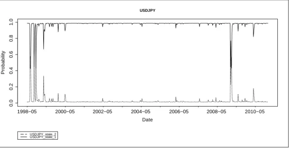
Tables (4) and (5) provide the detailed results relative to the foreign exchange rates between the Yen and Dollar. The market is characterized by a two-state regime : the return in the bull regime is equal to -1.08% whereas the volatility is equal to 10.503%. In the bear regime, the statistics are respectively -90.563% and 38.599%. Following the transition matrix, the bull regime appears to be the more persistent: the probability to be in regime 1 at time t if regime 1 prevails in the economy at time t − 1 is equal to 0.989. On the contrary, the state 2 is more volatil : the probability to move from regime 2 to regime 1 is closed to 0.43. Accordingly, the foreign exchange rates between the Yen against Dollar is characterized by a strong stability in the regime 1. Some crisis may induce a jump to the other regime but the market switches quickly to its initial status. Figure (3) illustrates this phenomenon.

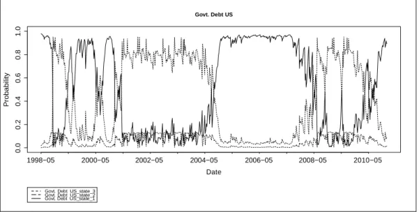
Tables (6) and (7) provide the results for the US government debt. US debt market is characterized by a three-state regime. States 1 and 3 correspond to the bear market with a negative return whereas the state 2 presents a return equals to 12.880%. For each state, the volatility is quite low, closed to 4%. We have to note that the volatility in the bull regime is higher than the volatility in the bear states. State 1 is the more persistent state with a transition probability equals to 0.989. When a crisis occurs, the market may switches to state 2 but this state appears to be a transitory state, the probability to be in the same state a time t + 1 being only equal to 0.85. The state 3 is quite curious. It appears unfeasible to stay in this state more than one period : p33 = 0. State 2 seems to be the more probable step after this state. Historically,

Figure (4) shows that state 3 has not occured.

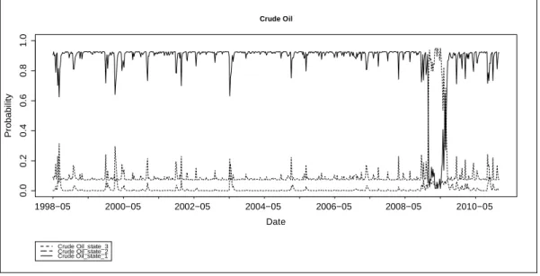
Crude Oil is also characterized by a three-state regime, two states corresponding to the bear market – negative average return – and one bullish regime – average return equals to 37.967% and volatility equals to 20.244%. Curiously, the state two

appears to be the more persistent regime, p22 = 0.95, in spite of of the fact it is the

more volatil – the variance of the state 2 return is equal to 0.81%. State 3 is the less persistent regime and if the state 3 prevails at time t in the economy, state 1 will the more probable state which will occur at time t + 1 : p31 = 0.73. According to

Figure (5), state 1 is the more frequent state which prevails in the economy. Even if p11 < p22 , this phenomenon may be explain by the fact that to move from state 1

to state 2, the market has to transit by state 3. On the contrary, if market is in the state 2, it may directly switch to state 1.

In terms of equities, Tables (10) and (11) show that the S&P index is characterized by a four-state regime. Two states correspond to the bullish regime (states 3 and 4) and two states stand for the bear market. The volatility is the highest for the state having the lowest average return. Accordingly with Figure (6) this state – state 1 – corresponds to a pure crisis regime. For example, this state prevailed at the beginning of the 2008 financial crisis. This state is quite persistent p11 = 0.83. But,

the more persistent state is the state 3, with p33 = 0.98. On the contrary, Table (11)

(11)

of the state 2 corresponds to the probability to move to the state 4, (p24 = 0.99).

Similarly, p42 = 0.56 and p44 = 0.43.

But, in addition to that, we have to consider two pairs of regimes, on the one hand the states 1 and 3, on the other hand the states 2 and 4. Indeed, when a state prevails in the economy, for example the state 2 or the state 4, it is very difficult to jump in the other block : p21 = 0.000, p23 = 0.003, p41 = 0.000 and p43 = 0.013. On

the contrary, p24 = 0.992, p42 = 0.560 and p44 = 0.427. Similar results are got if the

state

1 or 3 prevails. This results may be interpreted as follows : in “standard” conditions, returns fluctuates between two regimes. When a crisis occurs, the market switches from one block to the other. Anoter shock will be required to go back to the previous market conditions. This phenomenon is clearly illustrated in the Figure (6) which shows that the states 1 and 3 prevailed in the economy on the one hand between 1998 and 2004 and on the other hand beetween 2008 and 2010. Between 2004 and 2008, the states 2 and 4 drove the market.

4.3

4.3 4.3 Comparisons

Comparisons

The detailed results for the other assets of our sample are presented from table (12), page (18), to table (19), page (18). Parallels may be drawn between some asset classes. For example, the foreign exchange rate Swiss Franc against Dollar is characterized by a two-state regime, like the Yen. Moreover, characteristics of each state are very similar, both in terms of average return, volatility and transition probability. One state appears to be very persistent, with a probability to stay in the same state closed to 0.99. The other state corresponds to crisis phenomenons and is abso- lutly not persistent, the probability to switch being above 0.4.

On the contrary, FX Euro and GBP against Dollar present an additional state. That may be explained by the fact that Swiss Franc or Yen are ofter considered as safe haven by investors. Both EUR/USD and GBP/USD markets present two bear states and one bull regime. Volatility are similar. Nevertheless, EUR/USD presents only one very persistent state – state 3, p33 = 0.98, p11 and p22 being closed to 0.5

– whereas GBP/USD is characterized by two persistent states – p22 = 0.91 and p33

= 0.96.

In terms of bonds, two types of behaviours may be highlighted. First of all, both government and investment bonds are characterized by a three-states model whereas 5 or 6 states have to be considered for high yield bonds. Two bull regimes drive the returns of EU Government Debt and of the Investment Grade Debt US. On the contrary, two bull regimes may be noted for US Government and EU Investment Grade Debt. In each case, the volatility is very low, the variance being minus that 0.1%. Nevertheless, compared to the EU Investment Grade Debt, the US Investment Grade Debt is much more persistent. Chronology may be presented as follows. First of all, state 2 is very persistent : p22 = 0.94. But... it seems to be very difficult to

reach this state, because p12 = 0.013 and p32 = 0.000. Thus, market switches from

state 1 to state 3 and inversely, p13 = 0.23 and p31 = 0.73. Only a crisis may induce

a jump to the state 2. If similar results are got for the EU Investment Grade Debt, the transition probability are less closed to one or zero and then the regime changes are much more frequent. Figures (7) and (8) illustrate this point.

Equity indices are very homogeneous. Each index is characterized by a four-state regime, like S&P Index, excepted MSCI Asia Index. Moreover, each index presents two or three bear regimes. In addition to that, one very persistent state may be

(12)

(13)

highlighted. For example, for the Eurostoxx Index, the probability to stay in state two prevails in the economy, p22 , is 0.91. We get p33 = 0.93 for the MSCI Europe,

p0.93 for the MSCI Latin Amarica and p0.89 = 0.89 for the MSCI Europe Small Caps.

The same figures than for the S&P Index have to be highlighted. Two blocks of bull and bear regimes may be considered, the market sitching from one to the other through some major shocks. For example, Figures (9) and (10) provide the following chronology :

– in 1999, between 2001 and 2002, and from 2003 to 2008, state 1 prevailed in the Eurostoxx market.

– state 2 was mainly driving in the others periods.

– for the Small Caps, states 1 and 2 were mainly prevailing until 2008, the states 3 and 4 in 1998, in January 2002 and from 2008 to 2010.

5

5 5 Conclusion

Conclusion

In this paper, we show that contrary to a shared belief, more than two states generally explain asset return dynamics. In addition to that, the number of relevant states does not depend on the statistical properties of the underlying asset. Nevertheless, some parallels may be drawn between asset classes : bonds are characterized by the same number of states than exchange rates, equities having an additional state and high yield bonds presenting the highest number of states.

References

AMISANO, G. AND GIACOMI NI, R., 2007. Comparing Density Forecasts via Weighted Likelihood

Ratio Tests, Journal of Business and Economic Statistics, American Statistical Association, vol. 25, pages 177-190, April.

ANG, A. AND BEKAERT, G. (2002a): International Asset Allocation with Regime Shifts, Review of Financial Studies, 15, 1137U˝ 1187.

ANG, A. AND BEKAERT, G. (2002b): Regime Switches in Interest Rates, Journal of Business & Economic Statistics, 20, 163U˝ 182.

CHAUVET, M. AND PO TTER. S. (2000): Coincident and Leading Indicators of the Stock Market,

Journal of Empirical Finance, 7, 87U˝ 111.

HAMI LT ON, J.D., 1989. A New Approach to the Economic Analysis of Nonstationary Time Series

and the Business Cycle, Econometrica, Econometric Society, vol. 57(2), pages 357-84, March. MAHEU, J., MCCURDY, TH. AND SONG, Y. (2010): Components of Bull and Bear Markets: Bull

Corrections and Bear Rallies, Working Paper 402, University of Toronto.

NEWEY, W. K., WEST, K. D. (1987): A Simple, Positive Semidefinite, Heteroskedasticity and Au-

tocorrelation Consistent Covariance Matrix, Econometrica, 55, 703-708.

VUONG, Q. H. (1989): Likelihood Ratio Tests for Model Selection and Non-Nested Hypotheses,

Econometrica, Vol. 57, Iss. 2, 1989, pages 307-333.

(14)

A

A T

T

Tables

T

ables

ables and

and

and F

and

F

Figures

igures

Asset Asset Asset

Asset VolatilityVVVolatilityolatilityolatility AAAverageAverageverage returnveragereturnreturnreturn Sharpe ratioSharpeSharpeSharperatioratioratio SkewnessSkewnessSkewnessSkewness KKurtosisKKurtosisurtosisurtosis

Govt. Debt US 5.99% -36.41% -0.844 -0.01 0.05

SP500 19.89% -0.05% 0.000 -0.76 5.93

Russell 2000 24.83% 2.35% 0.013 -0.64 3.56

Investment Grade US 6.90% -35.89% -0.721 -0.24 2.28

High Yield US 9.43% -35.50% -0.522 -1.12 14.37

Govt. Debt EMU 4.52% -33.78% -1.036 -0.44 2.32

Eurostoxx 24.10% -1.39% -0.008 -0.77 5.83

MSCI Small Cap EMU 22.08% 2.68% 0.017 -1.47 7.41

Investment Grade EMU 4.06% -33.68% -1.150 -0.66 3.36

High Yield EMU 12.18% -34.61% -0.394 -1.52 11.35

Crude Oil 26.77% 7.94% 0.041 -0.70 2.83 DJ Commodity 17.53% 1.93% 0.015 -0.87 3.28 MSCI EM Asia 23.10% 5.96% 0.036 -0.45 2.03 MSCI EM Latam 25.14% 12.26% 0.068 -0.52 4.16 MSCI EM Europe 31.77% 9.62% 0.042 -0.31 7.90 USDCHF 10.61% -3.21% -0.042 -0.19 0.26 EURUSD 10.17% 1.45% 0.020 -0.23 0.90 USDJPY 12.26% -3.41% -0.039 -1.39 10.32 GBPUSD 9.75% -0.63% -0.009 -0.61 4.21

Table 1: Descriptive

Descriptive statistics

Descriptive

statistics

statistics of

of

of the

the

the returns

the

returns

returns on

on the

on

the

the assets

the

assets

assets considerend

considerend

considerend in

in

in the

the

dataset

The statistics presented in the table are computed using logarithmic returns over the period that starts on the 04/03/1998 and ends on the 12/31/2010. The data frequency is weekly. Both the standard deviation and the average returns are scaled into yearly quantities for the ease of their reading.

Mean

Median

Std.

Std. De

Std.

Dev

De

v

v....

v

Sk

Skewness

ewness

3 States

3.50

3

0.619

0.800 5 States

5.09

5

0.997 -0.129

Table 2: Monte

Monte

Monte Carlo

Carlo

Carlo test

test

test results

results

This table presents the results of the Monte Carlo experiments presented in Section 2.3. Two different specifications are used, one using 3 different regimes and another using 5 regimes. For each simulation, a sample of size of 650 weeks of trading is sampled. Using each of the 10 000 replications, we estimate the number of regime using the test presented in Section 2.2. The parameters used for these different models are presented in Section 2.3. The table presents the resulting average, median, standard deviation and skewness obtained from the 10 000 replications.

(15)

60.0% 50.0% 40.0% 30.0% 20.0% 10.0% 0.0% 1 ₂ 3 ₄ 5 ₆ 7 ₈ 9 10 5 States 3 States

3 States

5 States

Figure 1: F

F

Frequencies

requencies

requencies for

for each

for

each

each possible

possible

possible number

possible

number of

number

of

of regime

regime

regime obtained

regime

obtained

obtained with

with

with the

the

Monte

Monte Carlo

Carlo

Carlo simulations

simulations

This figure presents the results of the Monte Carlo experiments presented in Section 2.3. Two different specifications are used, one using 3 different regimes and another using 5 regimes. For each simulation, a sample of size of 650 weeks of trading is sampled. Using each of the 10 000 replications, we estimate the number of regime using the test presented in Section 2.2. The parameters used for these different models are presented in Section 2.3. The figure presents the resulting empirical probabilities of estimating a given number of regimes, given that the underlying model has either 3 or 5 regimes.

(16)

E st im at ed n u m b er o f re g im e s U S D C H F U S D JP Y G o v t. D e b t U S In v es tm e n t G ra d e U S G o v t. D e b t E M U In v e st m en t G ra d e E M U C ru d e O il D J C o m m o d it y M S C I E M A si a E U R U S D G B P U S D S P 5 0 0 R u ss e ll 2 0 0 0 E u ro st o x x M S C I S m al l C a p E M U M S C I E M L a ta m M S C I E M E u ro p e H ig h Y ie ld U S H ig h Y ie ld E M U

P

PARAMETERS

ARAMETERS

ARAMETERS ESTIM

ESTIM

ESTIMA

A

ATES

TES

Estimate

Std.

Std. De

De

Dev

De

v

v....

tttt----value

value

Expectation

45.5362

26.1348

1.7424

Standard Deviation

-2.3466

11.064 -0.2121

Sharpe ratio

-0.37017

2.6202

-0.1413

Skewness

-4.4045*

2.1936*

-2.0079*

Kurtosis

0.08024

0.2163

0.3709

THRESHOLDS

THRESHOLDS ESTIM

ESTIM

ESTIMA

A

ATES

TES

Estimate

Std.

Std. De

De

Dev

De

v

v....

tttt----value

value

2|3

1.4711

1.9966

0.7368

3|4

4.1991

2.2619

1.8565

4|5

6.8112

2.6375

2.5824

5|6

8.6196

2.8335

3.042 Table 3: Multivariate

Multivariate

Multivariate probit

Multivariate

probit

probit estimates

estimates of

estimates

of

of the

of

the

the factors

the

factors expla

factors

expla

explaining

expla

ining

ining the

ining

the

the number

the

number

number of

of

regimes

regimes in

in

in asset

asset

asset returns

returns

This table presents the results of a multivariate probit regression trying to explain the number of regimes implicit in asset returns. The top panel presents the estimates and their standard deviations whereas the bottom panel presents the estimated thresholds. * indicates a significantly different from zero estimate up to a 5% risk level.

Number of regimes 7 6 5 4 3 2 1 0 Assets

Figure 2: Estimated

Estimated

Estimated number

number

number of

of

of regime

regimes

regime

s

s in

in

in asset

asset

asset returns

returns

(17)

P ro b a b ili ty 0 .0 0 .2 0 .4 0 .6 0 .8 1 .0 Mean Volatility State 1 −1.076 10.503 State 2 −90.563 38.599

Table 4: JPY/USD

JPY/USD

JPY/USD market

market

market characteristics

characteristics –

characteristics

–

– in

–

in

in %

%

State 1 State 2 State 1 0.98859 0.01141

State 2 0.42627 0.57373

Table 5: JPY/USD

JPY/USD

JPY/USD transition

transition

transition matrix

transition

matrix

USDJPY

1998−05 2000−05 2002−05 2004−05 2006−05 2008−05 2010−05 Date

USDJPY_state_2

USDJPY_state_1

Figure 3: State

State

State probability

State

probability

probability for

for

for JPY/USD

JPY/USD

JPY/USD exchange

exchange rate

exchange

rate

rate from

rate

from

from 1998

from

1998 to

1998

to

to 2010

2010

(18)

P ro b a b il it y 0 .0 0 .2 0 .4 0 .6 0 .8 1 .0 Mean Volatility State 1 −0.796 3.639 State 2 12.880 4.469 State 3 −72.137 3.990

Table 6: US

US

US Government

Government

Government Debt

Government

Debt

Debt market

Debt

market characteristics

market

characteristics

characteristics –

characteristics

–

– in

in

in %

in

%

State 1 State 2 State 3 State 1 0.98857 0.01143 0.00000

State 2 0.00755 0.85724 0.13521

State 3 0.04630 0.95370 0.00000

Table 7: US

US

US Government

US

Government

Government Debt

Government

Debt

Debt transition

transition

transition matrix

transition

matrix

Govt. Debt US

1998−05 2000−05 2002−05 2004−05 2006−05 2008−05 2010−05 Date

Govt. Debt US_state_3

(19)

P ro b a b il it y 0 .0 0 .2 0 .4 0 .6 0 .8 1 .0 Mean Volatility State 1 37.967 20.244 State 2 −160.332 64.849 State 3 −229.603 28.453

Table 8: Crude

Crude

Crude Oil

Crude

Oil

Oil market

Oil

market

market characteristics

market

characteristics –

characteristics

–

– in

in

in %

%

State 2 0.01446 0.95081 0.03474

State 3 0.73075 0.02252 0.24672

Table 9: Crude

Crude

Crude Oil

Crude

Oil

Oil transition

transition

transition matrix

matrix

Crude Oil 1998−05 2000−05 2002−05 2004−05 2006−05 2008−05 2010−05 Date Crude Oil_state_3 Crude Oil_state_2 Crude Oil_state_1

Figure 5: State

State

State probability

State

probability

probability for

for

for Crude

Crude

Crude Oil

Oil from

Oil

from

from 1998

1998

1998 to

to 20

to

20 2010

20

10

(20)

P ro b a b ili ty 0 .0 0 .2 0 .4 0 .6 0 .8 1 .0 Mean Volatility State 1 −89.054 48.720 State 2 −31.375 10.888 State 3 1.825 18.782 State 4 35.972 8.240

Table 10: S&P

S&P

S&P market

market

market characteristics

characteristics –

characteristics

–

– in

in

in %

%

State 1 State 2 State 3 State 4 State 1 0.83453 0.00000 0.16547 0.00000

State 2 0.00000 0.00461 0.00336 0.99203

State 3 0.01657 0.00000 0.98034 0.00309

State 4 0.00000 0.56035 0.01306 0.42659

Table 11: S&P

S&P

S&P transition

S&P

transition

transition matrix

matrix

SP500 1998−05 2000−05 2002−05 2004−05 2006−05 2008−05 2010−05 Date SP500_state_4 SP500_state_3 SP500_state_2 SP500_state_1

(21)

State 2 0.49898 0.48578 0.01525

State 3 0.00003 0.01978 0.98019

State 2 0.08816 0.91184 0.00000

State 3 0.00000 0.03844 0.96156

Mean Volatility _{State 1} _{State 2}

State 1 −206.147 11.031 State 1 0.42218 0.57782

State 2 −1.661 10.305 _{State 2} _0.00442 _0.99558

Table 12:

CHF/USD CHF/USD CHF/USD CHF/USD exchange exchange exchange exchange rates rates rates rates market

marketmarket

market characteristicscharacteristicscharacteristicscharacteristics –––– ininin %in% %%

Table 13:

CHF/USDCHF/USDCHF/USDCHF/USD transitiontransitiontransition matrixtransitionmatrixmatrixmatrix

Mean Volatility State 1 47.118 6.019

State 2 −34.735 7.175

State 3 −9.857 13.651

Table 14:

EUR/USD EUR/USD EUR/USD EUR/USD exchange exchange exchange exchange rates rates rates rates market

marketmarket

Table 15:

EUR/USDEUR/USD transitionEUR/USDEUR/USD transitiontransition matrixtransitionmatrixmatrixmatrix

Mean Volatility State 1 −73.497 6.340

State 2 8.855 7.418

State 3 −17.968 21.643

Table 16:

GBP/USD GBP/USD GBP/USD GBP/USD exchange exchange exchange rates exchange rates rates rates market

marketmarket

Table 17:

GBP/USD GBP/USD GBP/USD GBP/USD transitiontransitiontransitiontransition matrixmatrixmatrixmatrix

State 2 21.342 13.721

State 3 −55.931 18.720

State 2 0.00246 0.81826 0.17929

State 3 0.00000 0.86652 0.13348

Table 18:

DJDJ CommodityDJDJ CommodityCommodity marketCommoditymarketmarketmarket charcharcharchar---- acteristics

acteristicsacteristics acteristics ––– in–ininin %%% %

Table 19:

DJ DJ DJ DJ CommodityCommodityCommodityCommodity transition transition transition transition matrix

matrix matrix matrix

(22)

State 1 0.29099 0.00000 0.00054 0.00000 0.70847 0.00000 State 2 0.00000 0.69959 0.04939 0.04253 0.00000 0.20849 State 3 0.44393 0.00000 0.46768 0.00000 0.00143 0.08696 State 4 0.00000 0.06210 0.00000 0.93789 0.00000 0.00001 State 5 0.00067 0.00000 0.87476 0.00000 0.12457 0.00000 State 6 0.00000 0.14786 0.00000 0.01937 0.00000 0.83277 Mean Volatility

State 1 −139.382 2.044

State 1 State 2 State 3

State 2 0.387 3.657

_{State 1} _0.0000 _0.00000 _1.00000

State 3 76.610 2.579

_{State 2} _0.0047 _0.99192 _0.00337

State 3 0.0000 1.00000 0.00000

Table 20:

EU EU GovernmentEU EU GovernmentGovernmentGovernment

Debt Debt Debt

Debt marketmarketmarketmarket characteristicscharacteristicscharacteristics –characteristics ––– in

in in in %%% %

Table 21:

EUEUEU GovernmentEUGovernmentGovernmentGovernment DebtDebt transitionDebtDebt transitiontransitiontransition matrixmatrixmatrixmatrix

State 2 2.569 9.929

State 3 −29.487 3.812

Table 22:

InvesmentInvesmentInvesmentInvesment Grade Grade Grade Grade US

US US

US Debt Debt Debt Debt market characterismarket characterismarket characterismarket characteris---- tics

tics tics

tics –––– ininin %in%%%

State 2 0.06064 0.93935 0.00001

State 3 0.73304 0.00000 0.26696

Table 23:

InvesmentInvesment Grade InvesmentInvesmentGrade Grade Grade USUSUS DebtUSDebt tranDebtDebt trantransitiontransitionsitionsition matrixmatrixmatrixmatrix

Mean Volatility

State 1 8.558 1.915

State 1 State 2 State 3

State 2 −1.636 4.900

State 1 0.81570 0.01753 0.16677

State 3 −11.656 2.096

_{State 2} _0.02902 _0.96520 _0.00578

State 3 0.36433 0.00455 0.63112

Table 24:

InvesmentInvesmentInvesmentInvesment GraGraGradeGradedede

Euro Euro Euro

Euro Debt Debt Debt marketDebt marketmarketmarket charactercharactercharactercharacter---- istics

istics istics

istics –––– ininin %in%%%

Table 25:

InvesmentInvesmentInvesmentInvesment Grade Grade Grade Grade EuroEuro DebtEuroEuro DebtDebtDebt transitiontransitiontransition matrixtransitionmatrixmatrix matrix

Mean Volatility State 1 4.821 2.296 State 2 −10.777 25.037 State 3 50.545 5.800 State 4 −28.583 5.816 State 5 21.617 2.667

Table 26:

High High YHigh High YYYiiiield eld USeld eld USUS Debt USDebt Debt Debt market

market market

market characteristicscharacteristicscharacteristicscharacteristics ––– in–ininin %%% %

State 1 State 2 State 3 State 4 State 5 State 1 0.96306 0.00000 0.00000 0.03693 0.00000

State 2 0.00000 0.93609 0.00000 0.06391 0.00000

State 3 0.05744 0.00000 0.62743 0.00000 0.31513

State 4 0.00345 0.01817 0.14142 0.80017 0.03679

State 5 0.02094 0.00000 0.06259 0.11617 0.80030

Table 27:

HighHigh YHighHigh YYYieldieldield USield US DebtUSUSDebtDebt transitionDebt transitiontransitiontransition matrixmatrixmatrixmatrix

State 2 1.173 2.983 State 1 State 2 State 3 State 4 State 5 State 6

State 3 −23.002 15.011

State 4 15.617 1.608

State 5 33.209 7.717

State 6 17.497 8.019

Table 28:

High High High High YYYield Yield ield Euro ield Euro Euro Euro Debt

Debt Debt

Debt marketmarketmarketmarket characteristicscharacteristicscharacteristicscharacteristics –––– in

in in in %%% %

(23)

Mean Volatility State 1 41.703 11.436 State 2 −7.397 24.787 State 3 −91.022 52.390 Mean Volatility State 1 211.271 10.588 State 2 21.555 14.706 State 3 −87.325 57.301 State 4 −64.051 21.639 State 1 −30.251 18.167 State 2 −67.684 59.653 State 3 56.296 13.548

State 2 0.06544 0.93456 0.00000 0.00000

State 3 0.10064 0.00000 0.89366 0.00570

State 4 0.60458 0.00003 0.17410 0.22129

Table 30:

MSCIMSCI AsiaMSCIMSCIAsiaAsiaAsia marketmarketmarketmarket charactercharactercharactercharacter----

istics istics istics

State 2 0.03636 0.95909 0.00455

State 3 0.00005 0.11152 0.88844

Table 31:

MSCIMSCIMSCIMSCI AsiaAsiaAsia transitionAsia transitiontransitiontransition matrixmatrixmatrix matrix

State 2 −26.741 41.953

State 3 −68.462 14.331

State 4 −139.275 12.436

Table 32:

EurostoxxEurostoxxEurostoxxEurostoxx marketmarketmarketmarket charactercharactercharactercharacter---- istics

istics istics

State 2 0.08459 0.91358 0.00184 0.00000

State 3 0.65235 0.00000 0.28291 0.06474

State 4 0.11022 0.35946 0.00000 0.53032

Table 33:

EurostoxxEurostoxxEurostoxxEurostoxx transitiontransitiontransitiontransition matrixmatrixmatrix matrix

State 2 −217.898 90.957

State 3 23.163 19.686

State 4 −399.324 21.566

Table 34:

MSCI MSCI MSCI MSCI EuropeEuropeEuropeEurope markemarkemarkemarketttt charcharcharchar---- acteristics

acteristics acteristics

acteristics –––– inininin %%%%

State 2 0.07924 0.85555 0.00000 0.06521

State 3 0.00000 0.00000 0.97435 0.02565

State 4 0.63463 0.11428 0.19584 0.05525

Table 35:

MSCIMSCI EuMSCIMSCI EuEuEuroperope transitionroperopetransitiontransition matrixtransitionmatrixmatrixmatrix

Mean Volatility

State 1 State 2 State 3 State 4 State 1 40.180 11.653

State 1 0.89323 0.10677 0.00000 0.00000

State 2 −72.676 17.906

State 2 0.20839 0.75297 0.03863 0.00000

State 3 −408.481 39.635

State 3 0.00000 0.00000 0.32453 0.67547

State 4 85.885 26.867

State 4 0.06049 0.00000 0.10178 0.83773

Table 36:

MSCI MSCI MSCI MSCI EuropeEuropeEuropeEurope Small Small Small Small Caps Caps Caps Caps

market market market

market characteristicscharacteristicscharacteristicscharacteristics –––– ininin %in%%%

Table 37:

MSCIMSCI EuropeMSCIMSCI EuropeEuropeEurope Small Small Caps Small Small Caps Caps Caps transittransittransition transition ion ion matrix

matrix matrix matrix

Table 38:

RusselRusselRusselRussel 2000200020002000 marketmarketmarketmarket characcharaccharac---- charac teristics

teristics teristics teristics ––– in–ininin %%% %

State 2 0.00002 0.93943 0.00000 0.06055

State 3 0.18875 0.00000 0.81125 0.00000

State 4 0.21557 0.00000 0.04144 0.74299

Table 39:

RusselRussel 2000RusselRussel200020002000 transitiontransitiontransition matrixtransitionmatrixmatrixmatrix

Mean Volatility

State 4 −2.634 29.193

Table 40:

Latin Latin Latin Latin AmericaAmericaAmericaAmerica marketmarketmarket charmarketcharcharchar---- acteristics

acteristics acteristics

(24)

P ro b a b ili ty P ro b a b il it y 0 .0 0 .2 0 .4 0 .6 0 .8 1 .0 0 .0 0 .2 0 .4 0 .6 0 .8 1 .0 Investment Grade US 1998−05 2000−05 2002−05 2004−05 2006−05 2008−05 2010−05 Date

Investment Grade US_state_3

Figure 7: State

State

State probability

probability

probability for

for

for Investment

for

Investment

Investment Grade

Investment

Grade US

Grade

US

US from

from

from 1998

from

1998 to

1998

to

to 2010

to

2010

Investment Grade EMU

1998−05 2000−05 2002−05 2004−05 2006−05 2008−05 2010−05 Date

Investment Grade EMU_state_3

(25)

P ro b a b ili ty P ro b a b il it y 0 .0 0 .2 0 .4 0 .6 0 .8 1 .0 0 .0 0 .2 0 .4 0 .6 0 .8 1 .0 Eurostoxx 1998−05 2000−05 2002−05 2004−05 2006−05 2008−05 2010−05 Date Eurostoxx_state_4 Eurostoxx_state_3 Eurostoxx_state_2 Eurostoxx_state_1