Parametric study of flow-induced vibrations in cylinder arrays under single-phase fluid cross flows using POD-ROM

HAL Id: hal-01825872

https://hal.archives-ouvertes.fr/hal-01825872

Submitted on 11 Dec 2019

HAL is a multi-disciplinary open access

archive for the deposit and dissemination of

sci-entific research documents, whether they are

pub-lished or not. The documents may come from

teaching and research institutions in France or

abroad, or from public or private research centers.

L’archive ouverte pluridisciplinaire HAL, est

destinée au dépôt et à la diffusion de documents

scientifiques de niveau recherche, publiés ou non,

émanant des établissements d’enseignement et de

recherche français ou étrangers, des laboratoires

publics ou privés.

Parametric study of flow-induced vibrations in cylinder

arrays under single-phase fluid cross flows using

POD-ROM

Elisabeth Longatte, Erwan Liberge, Marie Pomarede, Jean-François Sigrist,

Aziz Hamdouni

To cite this version:

Elisabeth Longatte, Erwan Liberge, Marie Pomarede, Jean-François Sigrist, Aziz Hamdouni.

Parametric study of flow-induced vibrations in cylinder arrays under single-phase fluid cross

flows using POD-ROM. Journal of Fluids and Structures, Elsevier, 2017, 78, pp.314-330.

�10.1016/j.jfluidstructs.2017.12.011�. �hal-01825872�

Parametric study of flow-induced vibrations in cylinder

arrays under single-phase fluid cross flows using POD-ROM

Elisabeth Longatte

a,

_*

_{, Erwan Liberge}

b

_{, Marie Pomarede}

a,b,c

_,

Jean-François Sigrist

c

, Aziz Hamdouni

b

a_{IMSIA, UMR EDF-ENSTA-CNRS-CEA 9219, 7 boulevard Gaspard Monge, 91120 Palaiseau, France}

b_{LaSIE, UMR 7356, CNRS-Université de La Rochelle, Avenue Michel Crépeau, 17042 La Rochelle cedex 1, France} c_{DCNS Research, 5 rue de l’Halbrane, 44340 Bouguenais, France}

Modeling numerically Flow-Induced Vibrations in heat exchangers at a microscopic scale requires high computational resources and time which are still unreachable. Therefore model reduction is investigated in the present work in order to address the issue of simulation computational time reduction. In the framework of POD-Galerkin projection methods, the purpose is to propose optimal a posteriori reduction strategies enabling error control on approximation as well as Reduced-Order Model (ROM) interpolation to deal with sensitivity analysis of solutions to parameter perturbations. A multi-phase fluid–solid POD-Galerkin-based method is proposed for modeling flows and vibrations in cylinder arrangements under single-phase fluid cross-flows. Moreover a single-POD basis method is evaluated in the context of ROM interpolation. This work is a first step in the development of robust ROM describing fluid and solid dynamics in the presence of turbulence, heat transfer effects and large magnitude structure displacements and deformations.

0. Introduction

Optimization of safety barrier reliability and Uncertainty Quantification (UQ) of physical models give rise to long-term research programs involving designers and engineers working on maintaining systems under operating conditions. The present article focuses on vibration risk assessment in heat exchangers in the context of lifecycle control and increase of mechanical components in spite of the very constrained conditions they are submitted to. In Pressurized Water Reactors (PWR) steam generators ensure the transition between the primary and secondary loops and are used to convert water into steam from heat produced by the core made of fuel assemblies. Each heat exchanger can measure up to 20 m and is made of regular confined arrangements of several thousands of thin elongated cylinders whose section diameter may be less than 2 cm. These cylinders are conveying the primary fluid and steam is produced, coming from the water on the shell side, so-called the secondary fluid. The heat exchanges take place at this stage in this area. Then the secondary steam is delivered to turbines for electric power generation. A brief dimensionless analysis of this geometrically complex system shows that as a first approximation under current conditions the dynamical behavior of these vibrating cylinders is independent on heat transfers. Therefore it is not necessary to account for thermal effects in the context of dynamical analysis. Due to geometry and to thermohydraulics conditions, most effects responsible for vibrations of cylinder arrays are due to Fluid Structure Interaction (FSI) and Flow-Induced Vibration (FIV) occurring at the external shell of the cylinders. They are due

*

Corresponding author.

to the hydrodynamic unsteady load exerted by the external fluid on these structures. Moreover the component is such that cylinders are submitted to two-phase flows at the top and to single-phase flows at the bottom. Therefore as a first step, in the present article, one focuses on single-phase FIV at the bottom of the heat exchanger where flows are crossing mostly transversally the array. The purpose is to address the multi-physics multi-scale issue of stability analysis of dynamical response of cylinder arrangements submitted to external single-phase fluid flows in order to be able to establish accurate stability maps applicable for design. Therefore parameter perturbations must be investigated in order to account for possible large variations of parameter values during the lifecycle of these mechanical components.

As far as numerical modeling is concerned, a fully three-dimensional microscopic-scale model of the bottom area of the heat exchanger tube array under single-phase fluid cross flow under real operating conditions characterized by Reynolds numbers of order of 105_{would lead to solving systems involving more than 10}10 _{degrees of freedom which} is still unreachable in practice even by using most advanced High Performance Computing (HPC) resources. Therefore superposition methods have been introduced in the context of first order asymptotic developments in order to perform linear stability analysis of these systems and exhibit major mechanisms involved in dynamical instability occurrence. Using space domain decompositions dimensionless parameter effects have been studied independently. Nevertheless HPC simulations performed on small-size domains are not yet convenient for design since they still require long computations of several hours to several days according to Reynolds numbers to be considered and to turbulence models to be involved. Therefore Reduced-Order Modeling (ROM) is investigated in order to deal with this problematic of reducing computational time. It is investigated in the present work by considering as a first step a two-parameter configuration where only Reynolds number and reduced velocity can vary while other parameters like mass ratio, Scruton number and pitch ratio of the cylinder arrangement are given. The basic idea is to use few High-Fidelity (HF) computations with a classical method (such as Finite Volumes and Finite Elements) to build low computational time models. Then ROMs have an initial cost, but this cost can be charged off if the models are used for large set of parametric values. The success of such approaches can be quantified by the large field of their applications. For example, ROMs have been used for studying different configurations of thermal management of data centers (Samadiani and Joshi, 2010), for controlling wave energy converters (Hesam and Shoori, 2014), fluid flow control at high Reynolds numbers (Semaan et al., 2016;Balajewicz et al., 2016) or in aeronautics (Kim, 2016). One way also explored is computation on smartphone, for which ROM approaches seem to be the appropriate solution. For example,

Modesto et al.(2015) proposed an application for smartphone for computing disturbances in the Barcelona harbor in quasi

real time using a ROM approach. On the same thing, ROM using a few/small resources could be used in a context of volunteer computing (Nouman Durrani and Shamsi, 2014) for a large parametric studies.

Few works exists on ROM development for FIV or FSI context. All works consist in adapting or extending the Proper Orthogonal Decomposition (POD) to this problematic. The POD is the most famous method for ROM in fluid mechanics and it has naturally been extended and adapted to the cases of flow in the presence of moving boundaries. For FSI cases similar to aeroelasticity, i.e where the fluid domain could be considered as fixed, the Navier–Stokes equations are linearized and projected on a POD basis (Barone et al., 2009b;Lieu et al., 2006). For small vibrations at the surface of the structure,Bourguet

et al.(2011) proposed a Hadamar formulation associated with a ROM-POD. For large fluid domain motion of deformation,

Rozza(2009) used POD on a parametric mesh and next built ROM for stationary problems on different meshes. In case of

imposed displacement of the structure,Balajewicz and Farhat(2014) proposed an immersed boundary ROM with a modified formulation. The ROM is directly built in an immersed boundary solver and is available only for imposed displacement of the solid domain. Among the previous proposed methods, none allows to solve a FSI problems with a large displacement of the structure, i.e cases where the fluid modifies the behavior of the structure, which interactively also changes the flow. The issue of using POD for moving domains deals with the paradox of computing a POD basis which is a spatial basis on a changing (i.e. a time-evolving) domain.Liberge and Hamdouni(2010) andLiberge et al.(2010) proposed a POD-multiphase formulation available for FSI problems with large displacement of the domain. The method consists in computing a POD basis of an interpolated velocity field on a reference grid, and next in projecting a multiphase formulation on this POD basis. It is recalled in the next section. This method has been successfully used for small and large displacements of a cylinder in a cross fluid flow for known parameters.

This paper explores the behavior of POD-multiphase ROM when the parameter values are different from those used to build the POD basis. In the first part, the principles of the POD, the POD-multiphase and the ROM parameter sensitivity analysis methods are explained. Next, the parameter sensitivity of the cylinder vibrations in a cross fluid flow is studied and results are discussed.

1. Theory

One considersΩ

⊂

R3such thatΩ

=

Ωf

(

t

) ∪

Ωs

(

t

) ∪

Γi

(

t

)

withΩsthe solid domain,Ωf the fluid domain andΓithe

fluid–solid interface. One defines the external boundary of the domain :Γf

= ∂

Ω

\

Γi. The normal vector n is oriented as

pointing out towards outside the solid domain. One defines a velocity field u over the whole domainΩ

× [

0

,

T

]

where T corresponds to the last time where the dynamics of the system is considered.

Fig. 1.Fluid structure interaction scheme.

1.1. The Proper Orthogonal Decomposition (POD)

The Proper Orthogonal Decomposition method being a well-known method, just a practical approach introduced by

Sirovich(1987) and the principal properties are exposed in the following. For more informations, one can refer toAllery et

al.(2004),Liberge and Hamdouni(2010) andLiberge et al.(2010).

Considering a set of M snapshots u

(

tk

) ,

k

=

1

· · ·

M of the velocity field, the POD method consists in solving the following

eigenvalue problem : CAk

= λ

kAk (1) with Cij

=

∫

Ωu

(

x

,

ti

)

u

(

x

,

tj

)

dx is a time correlation tensor of the snapshots of the velocity field. Next, the vectors of the

spatial basis are obtained with the decomposition :

Φk

(

x

) =

M

∑

m=1 Ak mu

(

x

,

tm

)

(x) (2)

The POD basis has the following properties :

•

There is a set of positive eigenvalues

(λ

i

)

i≥1which decreases to 0,

λ

1

≥ λ

2

≥ · · · ≥ λ

i

≥ · · ·

and

λ

i

→

0 (3)

and a set of vectors

(

Φi

)

i≥1which is a Hilbertian basis.

•

The vectors

(

Φi

)

are orthogonal and can be normalized:

(

Φi

,

Φj

) =

∫

Ω

Φi

(

x

) ·

Φj

(

x

)

dx

= δ

ij (4)

In case of an incompressible flow, the POD basis fulfills the free divergence, i.e. divΦi

=

0

,

i

≥

1.

•

The values of the temporal coefficients aiat specific times tk

,

k

=

1

· · ·

M are obtained from the projection of u onto

the basis :

ai

(

tk

) = (

u

(

tk

) ,

Φi

)

(5)

This procedure is called POD direct projection.

•

The eigenvalue

λ

iis the energy captured by the vectorΦi. For a given N, the POD decomposition is the best energy

decomposition that can be obtained.

Usually, in fluid mechanics, the POD is computed for the fluctuating velocity field u′_{and the POD basis is}

(

Φ_i′

)

.

1.2. The POD-multiphase formulation for FSI problems

The classical POD approach leads to a spatial basis, and needs fixed domains. Indeed, if the domainΩis time dependent, the eigenvalue problem(1)cannot be computed since the snapshots do not have the same domain definition at times tiand tj. To cancel this drawback,Liberge and Hamdouni(2010) andLiberge et al.(2010) have proposed to use a global domainΩ

with a fixed grid which recovers all the time variant domainsΩ

=

Ωf

(

t

) ∪

Ωs

(

t

) ∪

Γi

(

t

)

as displayed inFig. 2.

The method consists in computing snapshots using a classical Fluid Structure Interaction approach, which can use time variant grid. Next, the snapshots are interpolated from the time variant grid to the reference one. The snapshots can be

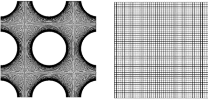
Fig. 2.Examples of grids for moving (left) and reference (right) domains to be introduced in order to account for time dependency of fluid–solid interface in a configuration involving a periodic cylinder arrangement with a moving central cylinder.

Fig. 3.Space- and time-dependent characteristic functions in the whole domain equal to 1 in the fluid and 0 in the solid domains for fluid and conversely for solid for coarse with 25×25 cells (left), refined with 50×50 cells (middle) and fine with 200×200 cells (right) cartesian grids for a two-dimensional configuration involving a periodic cylinder array.

computed by a classical solver using Arbitrary Lagrange Euler (ALE) method involving moving grid. Then a global velocity field is built onΩas follows:

u(x

,

t)

=

us(x

,

t)1Ωs(x

,

t)

+

uf(x

,

t)1Ωf(x

,

t) (6)

with us(x

,

t) the solid velocity field defined on spaceΩs(t) and uf(x

,

t) the fluid velocity field defined on spaceΩf(t) at time t. Characteristic functions are respectively expressed by 1Ωs(x

,

t) and 1Ωf(x

,

t) with 1Ωs(x

,

t)

=

1

−

1Ωf(x

,

t). Each function

1Ωi(for i

=

f or s) is defined by :

1Ωi(x

,

t)

=

{

1 if x

∈

Ωi(t)

0 else

Each variable (density and viscosity) and each field is decomposed following the example of Eq.(6).

Examples of time-dependent space distributions of characteristic functions are displayed in Fig. 3for several grid refinement.

1.3. Reduced-order dynamical model

Applying the POD to the velocity field(6)leads to a spatial basis defined onΩ.

We focus in this paper on cases where solid domain can be modeled using a rigid body coupled with springs and dampers. The non fluid constraints are expressed as external forcesF_fand momentaM_s.

Then, the ROM is built using the method proposed byLiberge and Hamdouni(2010). The principle is developed inLiberge

and Hamdouni(2010) and it is recalled in the present paper.

The formulation consists in extending the Navier–Stokes equations to the solid domain by adding a rigidity constraint Eq.(7)defined on the solid domain and a Lagrange multiplierΛassociated with the constraint as follows:

D(u)

=

0 inΩs(t) (7)

where D

(•)

is defined by :

D

(•) =

1

2

(∇ • +∇

T

_{•) .}

This leads to the following variational formulation on the global domainΩ:

HvΓ

=

{

u

|

u

∈

H1

₍

_Ω

_{) ,}

_u

₌

_u

H0

=

{

u

|

u

∈

H1

₍

_Ω

_{) ,}

_u

₌

_{0 on}

_∂

_Ω

_\

_Γ I

} ,

L20

(

Ω

) =

{

q

∈

L2

₍

_Ω

_{) |}

∫

Ωqdx

=

0

} ,

∀

u∗

_∈

_H 0and q

∈

L2

(

Ω

) ,

find u

∈

HvΓ

,

p

∈

L 2 0

(

Ω

) ,

Λ

∈

H1

(

Ωs

(

t

))

such that

∫

Ω

ρ

( ∂

u

∂

t

+

u

∇

u

)

u∗dx

−

∫

Ω p

∇ ·

u∗dx

+

∫

Ω q

∇ · v

dx

+

∫

Ω 2

µ

D

(

u

) :

D

(

u∗

)

dx

+

∫

Ωs(t) D

(

Λ

) :

D

(

u∗

)

dx

=

∫

Ω fu∗dx (8)

where

ρ

and

µ

are defined on the global domainΩ:

ρ = ρ

f

(

1

−

1Ωs

) + ρ

s1Ωs

, µ = µ

f

(

1

−

1Ωs

) + µ

s1Ωs

.

(9)

µ

sis the penalization factor associated with the Lagrange multiplier. f denotes the global volumique forces defined as

f

=

ff

(

1

−

1Ωs

) +

fs1Ωs (10)

where ff designates the standard external volumic hydrodynamic forces exerted by the fluid and fsis the other part of

external volumic forces acting on the rigid body different from fluid forces. fssatisfies the two following equations :

F_s

₌

∫

Ωs fsdx andMs

=

∫

Ωs fs

∧

xdx (11)

Next, the POD-ROM is built by choosing POD modesΦi

,

i

=

1

· · ·

N for the virtual velocity field and the decomposition of

uon the POD basis. For each n

=

1

, . . . ,

N:

⎧

⎪

⎪

⎪

⎪

⎪

⎨

⎪

⎪

⎪

⎪

⎪

⎩

N

∑

i=1 dai dtAin

+

N

∑

i=1 N

∑

j=1 aiajBijn

+

N

∑

i=1 aiCin

+

Dn

+

En

=

0 D

(

u

) =

0 inΩs

(

t

)

∂

1Ωs

∂

t

+

u

· ∇

1Ωs

=

0 (12) where : Ain

=

∫

Ω

ρ

Φi

·

Φndx Dn

=

∫

Ω 1ΩsTr

[

D(Λ)D(Φn)

]

dx Bijn

=

∫

Ω

ρ

(Φi

· ∇

)Φj

·

Φndx En

=

∫

Ω fΦndx Cin

=

2

∫

Ω

µ

Tr

[

D(Φi)D(Φn)

]

dx

As explained in Liberge and Hamdouni(2010) the formulation(12)does not need to compute explicitly the fluid forces on the structure because they are intrinsic to the formulation. In addition, the equivalent formulation using the fluctuating velocity field is described inAppendix A. Moreover the method can be extended to the case of deformable structure as described inAppendix B.

Remark.A POD-Galerkin method is involved in the present work. It is well-known that it can lead to instabilities, that is why the use of additional viscosities associated to each POD mode (Cazemier et al., 1998) or Least-Square approach (Tallet et al.,

2015;Carlberg et al., 2017) is often preferred in the context of fluid mechanics applications. However this is not necessary

in the present study since as explained in Liberge and Hamdouni(2010), the solid viscosity used to penalize the rigid body plays the role of the viscosity ofCazemier et al.(1998) and avoids instabilities.

2. Application to FIV of cylinder array 2.1. Configuration

In what follows, the model reduction method is applied to a configuration involving a periodic cylinder array made of one central moving cylinder and 8 truncated non-moving cylinders submitted to an external cross flow. The problem is two-dimensional thanks to the choice of parameters since the Reynolds number does not exceed 1000. Reduced velocity varies between 1 and 4. Other parameters are fixed. Pitch ratio is 1.44, Scruton number is taken to 0 and mass ratio equals 7.8. (SeeFig. 4).

These parameters are defined as follows: pitch ratio Pr

=

P

/

D with D the cylinder diameter and P the distance

between two centers of in-line neighbor cylinders in the square array; Scruton number or mass-damping parameter

Sc

= (

2

π ξ

m

) /(ρ

fD2

)

Fig. 4.Application to tube array.

mass ratio M

= ρ

f

/ρ

swith

ρ

sthe solid density; Reynolds number Re

=

(ρ

fUD

) /µ

with U the characteristic fluid flow

velocity and

µ

the kinematic fluid viscosity; reduced velocity UR

=

U

/

fsD with fsthe characteristic solid frequency in the

considered medium defined as fs

=

₂1_π

√

k

mand the stiffness of the spring.

The expression of fsdefined in Eq.(10)is :

f_s

=

k

|

Ωs

|

(

x

−

x₀

)

(13)

with

|

Ωs

|

the volume of the solid, and x0the solid position at rest. Thus,

F_s

(

t

) =

∫

Ωs(t)

fsdx

=

k

(

xG

(

t

) −

x0

)

(14)

with xGthe coordinate of the gravity center of the rigid body. For the studied case, ff

=

0.

Using the fluid, solid and geometric characteristics, the dimensionless formulation of system(8)leads to the definition of two significant nondimensional parameters, the Reynolds number and the reduced velocity. This leads to a nondimensional form for the ROM as follows:

for each n

=

1

, . . . ,

N,

⎧

⎪

⎪

⎪

⎪

⎪

⎪

⎨

⎪

⎪

⎪

⎪

⎪

⎪

⎩

N

∑

i=1 dai dt

˜

A

˜

in

+

N

∑

i=1 N

∑

j=1 aiajB

˜

ijn

+

N

∑

i=1 aiC

˜

in

+ ˜

Dn

+ ˜

En

=

0

˜

D

( ˜

u

) =

0 inΩ

˜

s

(˜

t

)

∂

1Ωs

∂ ˜

t

+ ˜

u

· ˜

∇

1Ωs

=

0 (15) where:

˜

Ain

=

∫

Ω h

( ˜

x

, ˜

t

) ˜

_Φi

· ˜

Φndx

˜

Dn

=

∫

Ω 1ΩsTr

[

_˜

D(Λ)D

˜

(_Φ

˜

_n)

]

dx

˜

Bijn

=

∫

Ω h

( ˜

x

, ˜

t

)

(_Φ

˜

_i

· ˜

∇

)_Φ

˜

_j

· ˜

Φndx

˜

En

=

1 M 4

π

2 U2 R

∫

Ω

( ˜

x

− ˜

xG

) ˜

Φndx

˜

Cin

=

2 Re

∫

Ω g

( ˜

x

, ˜

t

)

Tr

[

_˜

D(Φ

˜

i)D

˜

(Φ

˜

n)

]

dx

˜

Fig. 5.Velocity field in m.s−1_{for Reynolds number R}

E=612 and reduced velocity VR=1. Pitch ratio is 1.44, Scruton number is 0 and mass ratio 7.8.

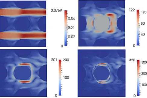
Fig. 6.Mean velocity field (top left), mode function shapes 1 (top right), 2 (bottom left) and 3 (bottom right) in m.s−1_{for Reynolds number R}

E=612 and

reduced velocity VR=1. The pitch ratio of the cylinder array is 1.44. Scruton number is 0 and mass ratio 7.8.

2.2. POD basis generation

For POD basis generation HF simulations are performed on this configuration for several values of Reynolds number and reduced velocity. With the previous approach, each set of parameter values corresponds to an optimal POD-ROM. In the fluid domain, the HF computation involves a FV solver with colocalized pressure and velocity fields and a fractional time step approach as described in Archambeau et al.(2004). An ALE formulation based on an elliptic equation for grid deformation is involved to account for solid wall motion and the solid dynamics is modeled by using an oscillator equation solved by using a Newmark time scheme. A relaxation is introduced in order to ensure the stability of the explicit solver used to describe the dynamics and kinematics boundary conditions at the time-dependent fluid structure interface. An example of flow velocity field is reproduced inFig. 5. This field was evaluated on the original reference grid. Then before ROM generation, it is interpolated on a cartesian coarser grid as displayed inFig. 1.

2.3. ROM accuracy and control

Results provided by the reduced-order models of FIV in cylinder arrangements are displayed below. An example of mean flow velocity u and first mode shapesΦ′i(for i

=

1 to 3) is plotted onFig. 6in a two-dimensional configuration involving a

periodic cylinder arrangement under cross flow. The mean flow velocity does not allow to capture the velocity of the rigid body. This velocity is captured using the following modes which are non zero on the area traveled by the cylinder. These modes are also needed to have the velocity fluctuations. For example, the mode 3 has to be used to capture the fluid flow and the solid velocity for cylinder position near the maximum amplitude.

Fig. 7.Expected values deduced from reference solution versus reduced-order model values of time coefficients ai(for i=1 to 3) deduced from computation

of the dynamical system for case ofFigs. 5and6.

Fig. 8. Predicted flow velocity field on the cartesian grid using the POD-ROM (left). Solid displacement (right): reference solution (dots) versus predicted solution (lines) for case ofFigs. 5and6.

Associated coefficients deduced from computation of the dynamical system(12)are displayed onFig. 7. The coefficients are compared to expected values according to the sample of reference solutions as follows (for i

=

1 to N):

a′_i

=

(u′

,

Φi′) (16)

Good adequacy has been found between the POD-ROM solution and the reference one. Finally the solution is reconstructed over the whole domain using the decomposition:

u(x

,

t)

=

u(x)

+

N

∑

n=1 a′ n(t)Φ′n(x)

The reconstruction of the solution is compared to the solution of the reference system over the interpolation domain. The flow velocity field as well as the solid displacement are displayed inFig. 8. With a truncate threshold fixed at 99%, the reduced order model solution reproduces reference values with a good agreement. The evolution of the relative error on the solution according to the mode number of the reduced model is given inFig. 9. 10 modes are sufficient to stabilize the error. The size of the ROM is very small compared with the HF model. The sensitivity to grid refinement is also investigated. When increasing the number of cells of the cartesian grid, the slope is improved and the accuracy of the model for a given mode number is better. For the present study,refine the grid more than a 50

×

50 grid does not improve the quality of the ROM.

TheFig. 3shows a good description of the geometry with this grid. As displayed inFig. 9, this grid is sufficient to capture the

physics of the phenomena.

2.4. ROM stability

The sensitivity to penalization factor is plotted onFig. 10. The stabilization compensates the effect of basis truncation which ensures a preservation of most energetic mode development but in the same time suppresses modes responsible for dissipation (Cazemier, 1997;Cazemier et al., 1998;Rempfer and Fasel, 1994). In the elementary configurations to be considered, an optimum is obtained for a solid viscosity close to the fluid value.

Fig. 9.Norm of the relative error on the solution according to number of modes of truncation from 1 to 30 (left) and to grid refinement for grids involving 25×25 to 200×200 cells (right) for case ofFigs. 5and6.

Fig. 10.Norm of relative error on the solution according to solid viscosity for case ofFigs. 5and6.

2.5. Performances and CPU time reduction

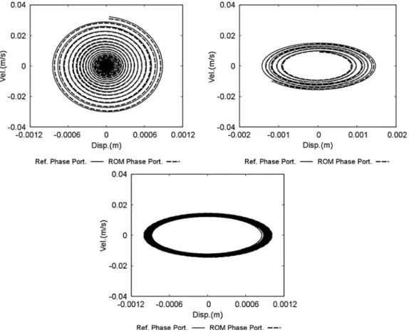
The predictive capability of ROM over a long period of time is pointed out in several configurations for a given Reynolds number and several values of reduced velocity. The phase portrait of the dynamical response is displayed inFig. 11in three cases: for reduced velocity below, close to and above the critical value of the system dynamical stability limit. In each case the solution predicted by the ROM is in good agreement with reference Bourguet et al.(2011) andBarone et al.(2009a).

In terms of computational time the gain is displayed onFig. 12. Comparisons of CPU times are performed by solving the ROM and High Fidelity (HF) model. In the present study, the HF model involves an ALE formulation of Navier–Stokes equations on a moving grid. The interpolation step from the moving grid to the reference grid as well as the POD basis computation are excluded. These two steps are considered as offline steps and only the online steps are compared. The gain in CPU time is expressed in % of gain per iteration, processor and cell. As shown inFig. 12, the gain of CPU time is about of a factor 100 in the present configurations.

3. Small ROM parameter perturbations 3.1. Principle of sensitivity analysis

Here it is proposed to study the behavior of the POD-ROM when one considers different values of parameters than those used to compute the POD basis. Considering the problem (Pλ):

Find u in space H for parameter

λ

such that :

⎧

⎨

⎩

∂

u

∂

t

=

f (u

, λ

) u(0)

=

u0 (17)

Fig. 11.Phase portrait of reference (lines) and ROM (dots) solutions for Reynolds number Re=612 and reduced velocity Ur=1 (top left), Ur=3.273 (top

right) and Ur=2.448 (bottom).

Fig. 12.Linear evolution of the gain in computational time compared to the reference simulation according to mode number of the reduced order model for case 3 ofFig. 11.

When a POD basis obtained for a parameter value

λ

0is used for a different value

λ

,Akkari et al.(2014b,a) proposed to bound the error by the number of POD modes involved in the POD-ROM :

Table 1

Parameter values used for ROM interpolation withλ1andλ2respectively the

Reynolds number and the reduced velocity of the problem. Case Values of POD basis ROM

parameters for generation generation

1 λ1 612 818 λ2 3.27 3.27 2 λ1 818 612 λ2 3.27 3.27 3 λ1 480 612 λ2 1.00 1.00 4 λ1 612 480 λ2 1.00 1.00 5 λ1 612 612 λ2 2.44 3.27 6 λ1 612 612 λ2 3.27 2.44 7 λ1 818 612 λ2 3.27 2.44

where uλis the approximation of the problem (Pλ) solution andu

˜

is given by :

˜

u

=

N

∑

n=1 aλ,λ0 n Φλn0 oru

˜

=

uλ,λ0

+

N

∑

n=1 a′ n λ,λ0 Φ′n λ0 ₍₁₉₎ aλ,λ0

n is obtained by solving the POD-ROM resulting from the projection of the problem (Pλ) Eq.(17)on

(

Φλ0

)

_.

It is expected that for parameter values not too far from

λ

0, the ROM provides an accurate solution for a number of POD vectors N not too big.

3.2. Numerical results

In what follows, pitch ratio, Scruton number and mass ratio are given and the system is characterized by two parameters : Reynolds number and reduced velocity. The purpose is to evaluate the influence of small variations of these both parameters on the accuracy of the reduced model. Values of Reynolds number and reduced velocity are changed and reduced order model associated to each case is used for other cases.

In the present study, the Reynolds number is modified by changing the inlet velocity, and the Reduced velocity by changing the inlet velocity and the spring stiffness. Therefore, the initial values of the aλ,λ0

n (or a′n

λ,λ0_{) time coefficients of}

the ROM have to be modified. We noteΓ the part ofΓf with non zero Dirichlet boundary condition, and xΓ a point of this

boundary. The Reynolds number and the reduced velocity can be written :

Re

=

ρ

fu

(

xΓ

)

µ

f UR

=

u

(

xΓ

)

fsD (20)

At the initial step, one gets :

uλ

(

xΓ

,

0

) =

uλ,λ0

(

xΓ

) +

N

∑

n=1 a′ n λ,λ0

₍

₀

₎

Φ′n λ0

₍

_x Γ

)

(21)

It is proposed to use a scaling coefficient

α

defined by :

α

(

λ, λ

0)

=

uλ_(x Γ

,

0) uλ0_(xΓ

_,

₀₎

.

(22) Then uλ,λ0

_{= α}

₍

_{λ, λ}

0)uλ0 (23) and a′ n λ,λ0

₍

₀

_{) = α}

₍

_{λ, λ}

0)a′n λ0

₍

₀

₎

₍₂₄₎

Several configurations for stable and unstable dynamical behaviors are considered. Values of parameters of the configu-rations to be considered are described inTable 1.

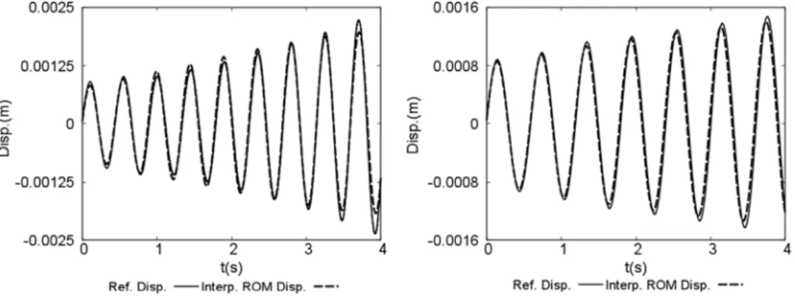
Fig. 13.Small perturbation of Reynolds number: case 1 (left), case 2 (right).

Fig. 14.Small perturbation of Reynolds number: case 3 (left), case 4 (right).

Fig. 15.Small perturbation of reduced velocity: case 5 (left), case 6 (right).

Three values of the Reynolds number are considered : 480,612 and 818. In that range of perturbation the flow regime is not changing. Three values are considered for reduced velocity too : a dynamical stable case (Ur

=

1), a second dynamical

stable case close to the critical stability (Ur

=

2

.

44) and an unstable case (Ur

=

3

.

27). Sensitivity to Reynolds number

deviation is displayed inFigs. 13and14respectively in dynamically unstable and stable cases. Reduced velocity deviation is investigated inFig. 15.

POD basis associated with stable case is used for prediction of unstable solution and conversely. Finally both parameters Reynolds number and reduced velocity are changed simultaneously inFig. 16. For each case, good behavior of the rigid body has been obtained by the ROM. It means that the ROM built for a parameter couple can be used for another near values

Fig. 16.Small perturbation of both Reynolds number and reduced velocity: case 7 with 10 (left) and 15 modes (right).

of parameters. In the case treated, the ROM is enough robust to model another behavior, i.e from stable to unstable or conversely. Change only one parameter or two in the same time does not affect the results. Increasing number of modes improves accuracy of results.

4. Conclusion

The multiphase-POD method has been applied for fluid structure interaction study in case of a 2D model of tube array. The proposed reduction method is efficient for velocity field prediction in a domain involving flows in interaction with solid dynamics. It relies on a standard POD-Galerkin projection method combined with an interpolation over a non-moving cartesian grid and a penalization method for dealing with heterogeneity of medium in the whole domain with possible unsteadiness. Both fluid and solid may feature a dynamical behavior. The robustness of the multiphase-POD methods is investigated in order to make possible real-scale real-time parameter sensitivity analysis and preserve the optimality of the generated ROM in terms of error control and computational time reduction. Good agreement has been found between the ROM solution and HF model, even if the ROM is used for another set of parameters than these used to build the POD basis. An extension of the method is now under development to account for turbulence and thermal effects.

Acknowledgments

This work was performed thanks to the support of DCNS Research, EDF R&D and CNRS. A special thank is addressed to Gaetan Mangeon at EDF R&D for its helpful contribution.

Appendix A. POD-Multiphase ROM for fluctuating velocity field

It has been observed that in fluid mechanics, the first POD mode is similar to the average velocity field and capture the most important part of the energy. Then, a practical approach consists in writing the POD-ROM for the fluctuating velocity field u′_{such as:}

u′(x

,

t)

=

u

(

x

,

t

) −

u

(

x

)

where u designates the mean flow velocity field and :

u′(x

,

t)

=

u′_s(x

,

t)1Ωs(x

,

t)

+

u

′

f(x

,

t)1Ωf(x

,

t)

A POD basis is computed for this field :

u′(x

,

t)

≃

N

∑

n=1

a′n(t)Φ′n(x) (25)

The Navier–Stokes equations for a domainΩi

,

i

=

f

,

s become :

⎧

⎪

⎪

⎨

⎪

⎪

⎩

ρ

i

∂

u′_i

∂

t

+ ρ

i

(

ui

∇

ui

+

ui

∇

u′i

+

u′i

∇

ui

+

u′i

∇

ui′

) − ∇ · σ

i

=

fiinΩi

∇ ·

ui

=

0 inΩi D(u)

=

0 inΩs(t) (26)

The same procedure as that presented in Section1.3leads to the following ROM: for each n

=

1

, . . . ,

N,

⎧

⎪

⎪

⎪

⎪

⎪

⎪

⎪

⎪

⎪

⎨

⎪

⎪

⎪

⎪

⎪

⎪

⎪

⎪

⎪

⎩

N

∑

i=1 da′ i dtA ′ in

=

N

∑

i=1 N

∑

j=1 B′_ijna′_ia′_j

+

N

∑

i=1 C_in′a′_i

+

D′_n

+

E_n′ D(u)

=

0 inΩs

∂

1Ωs

∂

t

+

u

· ∇

1Ωs

=

0 (27) with : A′_in

=

∫

Ω

ρ

Φ′i

·

Φ ′ ndx B′ ijn

= −

∫

Ω

ρ

(Φ′i

· ∇

)Φj′

·

Φn′dx C_in′

= −

∫

Ω

ρ

[

(u

· ∇

)Φi′

+

((Φ ′ i)

· ∇

)u

] ·

Φ ′ ndx

−

2

∫

Ω

µ

Tr

[

D(Φi′)D(Φ′n)

]

dx

−

2

∫

Γf

µ

D(Φ_i′)Φn′nd

γ

D′ n

= −

∫

Ω

ρ

(u

· ∇

)u

·

Φn′dx

−

2

∫

Ω

µ

Tr

[

D(u)D(Φn′)

]

dx

−

∫

Ω 1ΩsTr

[

D(Λ)D(Φ′n)

]

dx En′

=

∫

Ω 1ΩsfsΦn′dx where

ρ = ρ

f

(

1

−

1Ωs

) + ρ

s1Ωs

,

µ = µ

f

(

1

−

1Ωs

) + µ

s1Ωs

,

andΛis the Lagrange multiplier.

Appendix B. Multiphase formulation for deformable structure with small deformations

The case of a domain containing a fluid and a solid (with a linear elastic behavior) is considered. The aim is to propose a monolithic formulation of the system. Small deformations of the solid are superposed by large displacements of a rigid solid. The extension to large deformations and large displacements of the solid are considered in Favrie et al.(2009).

The solid is first considered as a structure with viscoelastic characteristics. AsHachem et al.(2010) andEl Feghali et al.

(2010) propose, one can write a monolithic formulation of Navier–Stokes equations inΩ.Hachem et al.(2010) and El Feghali et al. are interested by this monolithic formulation in the framework of finite-element models.

If one considers the equation governing the fluid domain, one gets the classical incompressible Navier–Stokes equations:

⎧

⎨

⎩

ρ

f

∂

uf

∂

t

+ ρ

f(uf

· ∇

uf)

− ∇ · σ

f

=

ff inΩf

∇ ·

uf

=

0 inΩf (28)

with associated boundary conditions, where

ρ

fis the fluid density, pfthe fluid pressure term and

σ

fthe stress tensor in the

fluid part, defined by:

σ

f

= −

pfId

+

2

µ

fD(uf) (29)

µ

fis the fluid dynamical viscosity and Idrepresents the identity tensor and D(uf) is the deformation rate tensor, itself defined

by D(uf)

=

1₂

(∇

uf

+ ∇

Tuf

)

The solved equation in the solid for uswith us(t)

=

∂_∂d_t, where d is the solid displacement, is:

ρ

s

∂

us

∂

t

+ ρ

s(us

· ∇

us)

− ∇ · σ

s

=

fs inΩs (30)

ρ

sis the solid density. The solid stress tensor

σ

sis defined by:

σ

s

=

2

α

D(d)

+ β

Tr(D(d))Id (31)

where

α

and

β

are the Lamé constants. This leads to its time derivate form

σ

˙

s:

˙

σ

s

=

2

α

D(us)

+ β

Tr(D(us))Id (32)

If we consider the hypothesis of small deformations, we can define the linearized Lagrangian deformation rate tensor as:

D(us)

=

1

2(

∇

us

+ ∇

T_u

s) (33)

To Eqs.(28)and(30), we have to add continuity equations for velocity and stress fields (n the external normal unity vector):

{

us|Γ_i

=

uf|Γ_i

σ

s|Γ_i

·

n

= −σ

f|Γ_i

·

n

(34)

We can choose to rewrite Eq.(32)as:

˙

σ

s

=

2

α

D(us)

− ˙

psId (35)

withp

˙

s

= −β

Tr(D(us))Idand we note

˙τ =

2

α

D(us). By coupling Eqs.(28)and(30)and with the stress tensors definition, we

deduce the following total strong formulation:

⎧

⎪

⎪

⎪

⎨

⎪

⎪

⎪

⎩

ρ

∂

u

∂

t

+ ρ

(u

· ∇

u)

− ∇ ·

(

−

pId

+

2

µ

f1ΩfD(u)

+

1Ωs

τ

)

=

f inΩ

∇ ·

u

+

1

κ

p

˙

s

= ∇ ·

u

+

1

κ

[ ∂

ps

∂

t

+

u

∇

ps

] =

0 inΩs (36)

where p

=

pf1Ωf

+

ps1Ωsand

κ =

1Ωs

β

,

κ

represents a compressibility coefficient.

Taking into account Eq.(36), a total weak form of Navier–Stokes equations inΩreads: Find u

∈

H(Ω), p

∈

L2(Ω) and

τ ∈

L2(Ω)N×N _{such as:}

_∀

_u∗

_{∈ {}

_v

_|

_v

_∈

_H(Ω)

_,

_u

₌

_{0 on}

_∂

_Ω

_\

_Γ

i

}

and for q

∈

L20(Ω)

= {

r

∈

L2(Ω)

|

∫

Ωrdx

=

0

}

:

⎧

⎪

⎪

⎪

⎪

⎪

⎪

⎪

⎪

⎪

⎨

⎪

⎪

⎪

⎪

⎪

⎪

⎪

⎪

⎪

⎩

∫

Ω

ρ

∂

u

∂

tu ∗_dx

₊

∫

Ω (u

· ∇

u)

·

u∗dx

−

∫

Ω p

∇ ·

u∗

−

2

∫

Ω

µ

f1ΩfD(u)

:

D(u ∗_)dx

−

∫

Ω 1Ωs

τ :

D(u ∗_)dx

₌

∫

Ω f u∗dx

∫

Ω

∇ ·

uqdx

+

∫

Ω 1

κ

[ ∂

ps

∂

t

+

u

∇

ps

]

qdx

=

0 (37)

El Feghali et al.(2010) choose to introduce a viscosity

µ

sin the solid as a penalization term. Thus, this equation becomes:

⎧

⎪

⎪

⎪

⎪

⎪

⎪

⎪

⎪

⎪

⎨

⎪

⎪

⎪

⎪

⎪

⎪

⎪

⎪

⎪

⎩

∫

Ω

ρ

∂

u

∂

tu ∗_dx

₊

∫

Ω (u

· ∇

u)

·

u∗dx

−

∫

Ω p

∇ ·

u∗

−

2

∫

Ω

µ

D(u)

:

D(u∗)dx

−

∫

Ω 1Ωs

τ :

D(u ∗_)dx

₌

∫

Ω f u∗dx

∫

Ω

∇ ·

uqdx

+

∫

Ω 1

κ

[ ∂

ps

∂

t

+

u

∇

ps

]

qdx

=

0 (38)

where

µ = µ

s1Ωs

+ µ

f(1

−

1Ωs). In the case of the POD, trial functions u∗are the POD modes. Global velocity and pressure

fields are decomposed along space and time as:

⎧

⎪

⎪

⎪

⎪

⎨

⎪

⎪

⎪

⎪

⎩

u(x

,

t)

=

N

∑

n=1 an(t)Φn(x) p(x

,

t)

=

M

∑

m=1 bm(t)Ψm(x) (39)

whereΦn,Ψmare elements of POD basis respectively for the velocity and the pressure fields for each n and each m, and an(t), bm(t) are time coefficients. The final low-order dynamical system is the following, for eachΦi, i

=

1

, . . . ,

N and eachΨi, i

=

1

, . . . ,

M:

⎧

⎪

⎪

⎪

⎪

⎨

⎪

⎪

⎪

⎪

⎩

N

∑

n=1 dan dt Ani

+

N

∑

n=1 N

∑

l=1 analCnliu

−

M

∑

m=1 bmBp1,mi

−

2 N

∑

n=1 anBu1,ni

−

2 N

∑

n=1

∫

t 0 an(s)ds Bu2,ni

=

Ei inΩ (40a) N

∑

n=1 anBp2,ni

+

M

∑

m=1 dbm dt B κ mi

+

N

∑

n=1 M

∑

m=1 anbmCnmip

=

0 (40b)

with the system coefficients:

Ani

=

∫

Ω

ρ

Φn

·

Φidx Cnliu

=

∫

Ω (Φn

· ∇

Φl)

·

Φidx Bp_1,mi

=

∫

Ω Ψm

∇ ·

Φidx Bu1,ni

=

∫

Ω

µ

D(Φn)

:

D(Φi)dx Bu 2,ni

=

∫

Ω

α

1ΩsD(Φn)

:

D(Φi)dx Ei

=

∫

Ω fΦidx Bp_2,ni

=

∫

Ω (

∇ ·

Φn)

·

Ψidx Bκmi

=

∫

Ω 1

κ

Ψm

·

Ψidx C_nmip

=

∫

Ω 1

κ

(Φn

· ∇

Ψm)

·

Ψidx

Taking into account the viscoelastic characteristic of the solid, this formulation has the advantage to offer a quasi-classical Navier–Stokes dynamical system to solve, with only a penalization term for the solid viscosity, and the introduction of

τ

leads to an integro-differential equation.

References

Akkari, N., Hamdouni, A., Liberge, E., Jazar, M., 2014a. A mathematical and numerical study of the sensitivity of a reduced order model by POD for a 2D incompressible fluid flow. J. Comput. Appl. Math. 270, 522–530.

Akkari, N., Hamdouni, A., Liberge, E., Jazar, M., 2014b. On the sensitivity of the POD technique for a parameterized quasi-nonlinear parabolic equation. Adv. Model. Simul. Eng. Sci. 1 (1), 1.

Allery, C., Guerin, S., Hamdouni, A., Sakout, A., 2004. Experimental and numerical POD study of the Coanda effect used to reduce self-sustained tones. Mech. Res. Commun. 31, 105–120.

Archambeau, F., Mechitoua, N., Sakiz, M., 2004. Code Saturne: a finite volume code for the computation of turbulent incompressible flows. Industrial applications. Int. J. Finite Vol. 1.

Balajewicz, M., Farhat, C., 2014. Reduction of nonlinear embedded boundary models for problems with evolving interfaces. J. Comput. Phys. 274, 489–504. Balajewicz, M., Tezaur, I., Dowell, E., 2016. Minimal subspace rotation on the Stiefel manifold for stabilization and enhancement of projection-based reduced

order models for the compressible Navier-Stokes equations. J. Comput. Phys. 321, 224–241.

Barone, M.F., Kalashnikova, I., Brake, M.R., Segalman, D.J., 2009a. Reduced order modeling of fluid structure interaction, Sandia Report - SAND2009-7189. Barone, M.F., Kalashnikova, I., Brake, M.R., Segalman, D.J., 2009b. Reduced Order Modeling of Fluid/structure Interaction. sand2009-7189, Sandia National

Laboratories.

Bourguet, R., Braza, M., Dervieux, A., 2011. Reduced-order modeling of transonic flows around an airfoil submitted to small deformations. J. Comput. Phys. 230 (1), 159–184.

Carlberg, K., Barone, M., Antil, H., 2017. Galerkin v. Least-squares Petrov-Galerkin projection in nonlinear model reduction. J. Comput. Phys. 330, 693–734.

Cazemier, W., 1997. Proper Orthogonal Decomposition and Low Dimensional Models for Turbulent Flows. Ph.D. Report.

Cazemier, W., Verstappen, R.W., Veldman, A.E.P., 1998. Proper orthogonal decomposition and law dimensional models for driven cavity. Phys. Fluids 10 (7), 1685–1699.

El Feghali, S., Hachem, E., Coupez, T., 2010. Monolithic stabilized finite element method for rigid body motions in the incompressible navier-stokes flow. Eur. J. Comput. Mech. - Fluid Struct. Interact. 19, 549–575.

Favrie, N., Gavrilyuk, S.L., Saurel, R., 2009. Solid-fluid diffuse interface model in cases of extreme deformations. J. Comput. Phys. 228, 6037–6077. Hachem, E., Rivaux, B., Kolczko, T., Digonnet, H., Coupez, T., 2010. Stabilized finite element method for incompressible flows with high Reynolds number. J.

Comput. Phys. 229, 8643–8665.

Hesam, J., Shoori, E., 2014. An Approach to Reduced-Order Modeling and Feedback Control For Wave Energy Converters (Masters thesis), Oregon State University.

Kim, T., 2016. Parametric model reduction for aeroelastic systems: Invariant aeroelastic modes. J. Fluids Struct. 65, 196–216.

Liberge, E., Hamdouni, A., 2010. Reduced-order modelling method via proper orthogonal decomposition for flow around an oscillating cylinder. J. Fluids Struct. 26, 292–311.

Liberge, Erwan, Pomarede, Marie, Hamdouni, Aziz, 2010. Reduced-order modelling by POD-multiphase approach for fluid-structure interaction. Eur. J. Comput. Mech. 19 (1–3), 41–52.

Lieu, T., Farhat, C., Lesoinne, M., 2006. Reduced-order fluid/structure modeling of a complete aircraft configuration. Comput. Methods Appl. Mech. Engrg. 195 (41–43), 5730–5742.

Modesto, D., Zlotnik, S., Huerta, A., 2015. Proper generalized decomposition for parameterized Helmholtz problems in heterogeneous and unbounded domains: Application to harbor agitation. Comput. Methods Appl. Mech. Engrg. 295, 127–149.

Nouman Durrani, M., Shamsi, J.A., 2014. Volunteer computing: requirements, challenges, and solutions. J. Netw. Comput. Appl. 39 (1), 369–380 cited By 13. Rempfer, D., Fasel, H.F., 1994. Evolution of three-dimensional coherent structures in a transitional flat plate boundary layer. J. Fluid Mech. 275, 257–283. Rozza, G., 2009. Reduced basis methods for stokes equations in domains with non-affine parameter dependence. Comput. Vis. Sci. 12 (1), 23–35. Samadiani, E., Joshi, Y., 2010. Reduced order thermal modeling of data centers via proper orthogonal decomposition: A review. Internat. J. Numer. Methods

Heat Fluid Flow 20 (5), 529–550.

Semaan, R., Kumar, P., Burnazzi, M., Tissot, G., Cordier, L., Noack, B.R., 2016. Reduced-order modelling of the flow around a high-lift configuration with unsteady Coanda blowing. J. Fluid Mech. 800, 72–110.

Sirovich, L., 1987. Turbulence and the dynamics of coherent structures. Quart. Appl. Math. 45 (3), 561–590.

Tallet, A., Allery, C., Leblond, C., Liberge, E., 2015. A minimum residual projection to build coupled velocity–pressure POD–ROM for incompressible Navier– Stokes equations. Commun. Nonlinear Sci. Numer. Simul. 22 (1–3), 909–932.