HAL Id: pastel-00982312
https://pastel.archives-ouvertes.fr/pastel-00982312
Submitted on 23 Apr 2014
HAL is a multi-disciplinary open access
archive for the deposit and dissemination of sci-entific research documents, whether they are pub-lished or not. The documents may come from
L’archive ouverte pluridisciplinaire HAL, est destinée au dépôt et à la diffusion de documents scientifiques de niveau recherche, publiés ou non, émanant des établissements d’enseignement et de
geometrical parts
Steffen Klonk
To cite this version:
Steffen Klonk. Numerical modelling of induction heating for complex geometrical parts. Other. Ecole Nationale Supérieure des Mines de Paris, 2013. English. �NNT : 2013ENMP0077�. �pastel-00982312�
MINES ParisTech
École doctorale n° 364 : Sciences fondamentales et appliquées
présentée et soutenue publiquement par
Steffen KLONK
le 16 décembre 2013
Modélisation Numérique du Chauffage par Induction
de Pièces à Géométrie Complexe
Doctorat ParisTech
T H È S E
pour obtenir le grade de docteur délivré par
l’École nationale supérieure des mines de Paris
Spécialité “Mécanique numérique”
Directeur de thèse : François BAY
T
H
È
S
E
JuryM. Egbert BAAKE, Prof., Institut für Elektroprozesstechnik, Leibniz Universität Hannover Rapporteur
M. Rachid TOUZANI, Prof., Laboratoire de Mathématiques, Université Blaise Pascal Rapporteur
M. Fabrizio DUGHIERO, Prof., Dipartimento di Ingegneria Industriale, Università di Padova Examinateur
Mme Annie GAGNOUD, Dr., Laboratoire SIMAP Groupe EPM, CNRS Examinateur
I Introduction 5
I.1 Structure of this document . . . 6
I.2 Induction heat treatment . . . 7
I.3 Industrial induction heating of a crankshaft . . . 9
I.4 Metallurgical aspects of hardening . . . 11
I.5 Major physical phenomena . . . 15
I.5.1 Skin effect . . . 15
I.5.2 Magnetic permeability and Curie temperature . . . 19
II Numerical model for induction heating 23 II.1 Physical model . . . 24
II.1.1 Maxwell’s equations . . . 24
II.1.1.1 E-H-J formulation . . . 26
II.1.1.2 A-V formulation . . . 27
II.1.2 Heat transfer equations . . . 28
II.2 Numerical model . . . 29
II.2.1 Classification of PDEs . . . 29
II.2.1.1 Elliptic PDEs . . . 30
II.2.1.2 Parabolic PDEs . . . 31
II.2.1.3 Hyperbolic PDEs . . . 32
II.2.2 Solution methods and discretisation . . . 35
II.2.2.1 Weak form of the voltage potential problem . . . . 37
II.2.2.2 Weak form of the heat transfer equation . . . 38
II.2.2.3 Weak form of the magnetic vector potential equation 39 II.2.3 Finite element spaces . . . 41
II.2.4 Existence and uniqueness . . . 44
II.2.5 Stable time discretisation and weak coupling procedure . . . 46
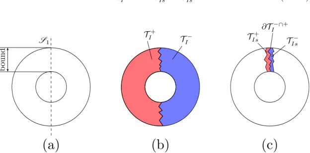
II.3 Computation of conforming source currents . . . 51
II.3.1 Two cutting plane current computation technique . . . 53
II.3.2 Tree gauging method . . . 58
II.3.3 Current potential formulation . . . 61
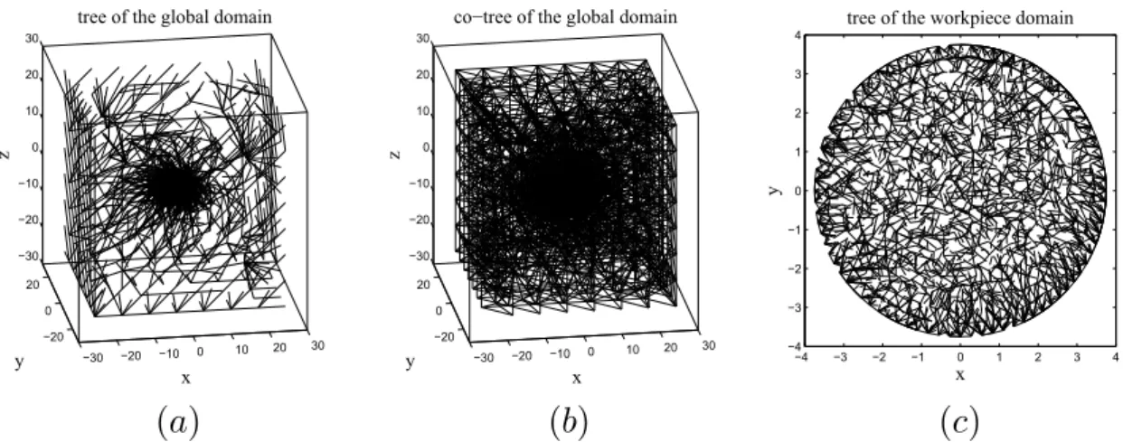
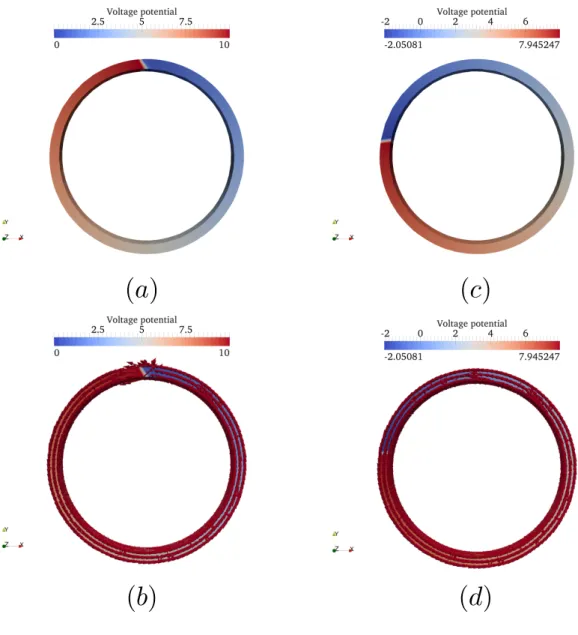
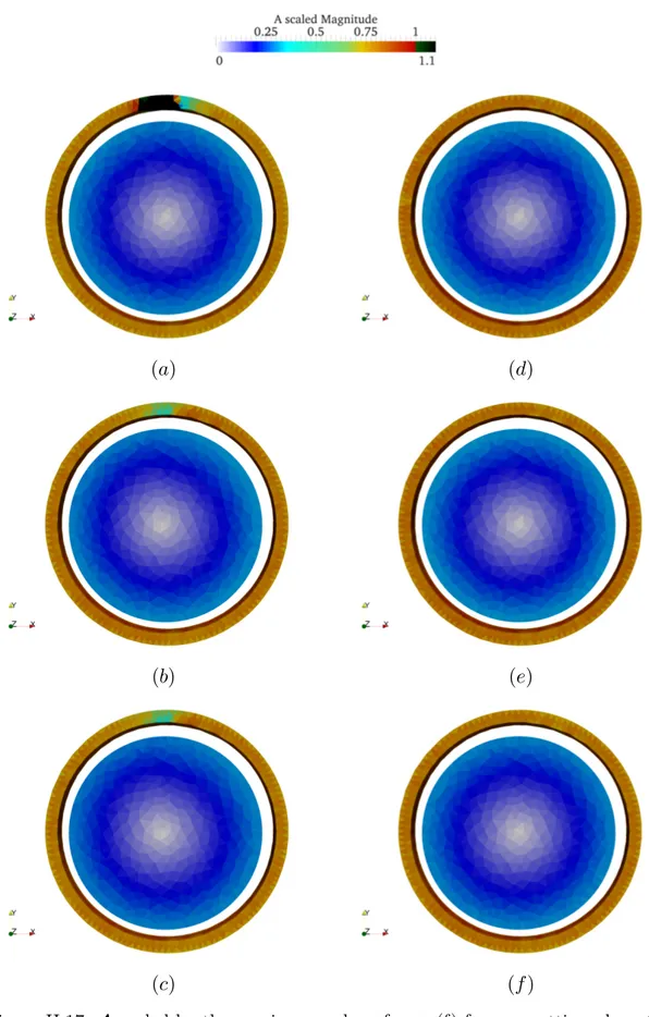
II.3.4 Benchmark application for a ring inductor test case . . . 62
III Efficient linear solvers for the associated electromagnetic problem 71 III.1 Requirements . . . 73
III.2 Preconditioners . . . 77
III.2.1 Classical preconditioners . . . 77
III.2.2 Stable decomposition of H0(curl, Ω) . . . 79
III.2.2.2 Auxiliary nodal space method with discrete elliptic
operators . . . 83
III.2.2.3 Auxiliary nodal space method with variationally equivalent elliptic operators . . . 84
III.2.2.4 Discretisation of Nh and Gh . . . 84
III.3 Multigrid methods . . . 86
III.3.1 Coarsening techniques . . . 88
III.3.1.1 Requirements . . . 88 III.3.1.2 RS, RS2 and RS3 . . . 90 III.3.1.3 CLJP . . . 91 III.3.1.4 Falgout . . . 91 III.3.1.5 PMIS . . . 92 III.3.1.6 HMIS . . . 93 III.3.1.7 ECGC . . . 94 III.4 Application . . . 95
III.4.1 Impact of coarsening type on convergence behaviour . . . 95
III.4.2 Impact of coarsening type on setup and solver setup time . . 99
III.4.3 Impact of coarsening threshold on convergence behaviour . . 102
III.4.4 Impact of operator ordering on convergence behaviour . . . . 104
III.4.5 Impact of material parameter distribution on convergence behaviour . . . 105
IV Modelling inductor motion 109 IV.1 Problem statement . . . 110
IV.2 Existing methods . . . 111
IV.3 Inductor motion using discrete level set functions . . . 115
IV.4 Application . . . 123
V Industrial applications 131 V.1 Cylinder spin hardening . . . 133
V.2 Gearwheel spin hardening . . . 138
V.3 Automotive crankshaft . . . 149
VI Conclusions 167 VI.1 Numerical model and industrial applications . . . 168
VI.2 Efficient linear solvers for the associated electromagnetic problem . 169 VI.3 Modelling inductor motion . . . 171
Français:
Le chapitre suivant introduit le sujet du chauffage par induction. Il donne un aperçu de la structure du document et des idées principales. On introduit le problème du chauffage par induction à l’égard de son application industrielle concernant un vile-brequin pour l’industrie automobile. Ensuite, on donne un bref aperçu des aspects métallurgiques et des phénomènes physiques qui ont lieu pendant le traitement thermique.
English:
The following chapter introduces the topic of induction heating. It gives an over-view of the structure of the document and the main ideas of this work. It introduces the problem of industrial induction heating, with respect to its application to the surface heat treatment of an automotive crankshaft. Afterwards, a brief overview is given of the metallurgical aspects and the physical phenomena that are taking place during the heat treatment procedure.
I.1 Structure of this document
The current chapter gives an overview of the induction heating process for com-plex geometrical parts. The main example in this work deals with an automotive crankshaft in the context of the industrial research project OPTIPRO-INDUX. This chapter outlines the metallurgical aspects of heat treatment, as well as the major physical phenomena, which affect the heat treating procedure. The physical phenomena, as well as the metallurgical aspects are very well known. The metal-lurgical aspects are given in great detail in [Barralis and Maeder, 1997], which has been referred to extensively in section I.4. Both the equilibrium diagram, shown in figure I.5, as well as the transformation diagram, presented in figure I.6, have been reproduced from the above-mentioned source. The experimental data for the given materials, as well as the main ideas of the theoretical concepts regarding induction heating in section I.5 can be found in [Rudnev, 2003]. These sources will not be cited again in these subsections, for reasons of brevity and readability. Additional sources complementing the former are identified.
Chapter II details the numerical model of the induction heat treatment process, including the fully transient eddy current model, the introduction of voltage po-tentials on closed inductor domains, as well as the heat diffusion model. It gives the reasoning behind the choice of the weak coupling procedure between electro-magnetic and heat transfer computation and specifies the implementation of this coupling procedure.
The numerical model of the induction heating process features a coupled multi physics model that results in a linear system of equations, involving millions of un-knowns that has to be solved in parallel with efficient numerical solvers. Chapter III presents the auxiliary space Maxwell multigrid method that is implemented for the industrial test case presented in this work. It is an algebraic multigrid precondi-tioner that decreases the residual error very efficiently in each iteration using suit-able finite element spaces and projection operators. The theoretical background, as well as details regarding the implementation of this parallel preconditioner are given. This is followed by an application test case, including a demonstration of the advantages and shortcomings of several preconditioner combinations.
Chapter IV details a new method for the introduction of the relative movement between inductor and crankshaft, based on a discrete level set function approach. It includes the application of the method with respect to the inductor rotation around an automotive crankshaft for a large scale test case.
Chapter V gives several applications of the induction heating model for different test cases, followed by the numerical treatment of an industrial crankshaft. The crankshaft model is provided by industrial partner PSA Peugeot Citroën and in-cludes an inductor provided by EFD Induction. The material for the crankshaft is provided by ASCOMETAL.
Finally, chapter VI sums up the key results of this work and gives an outlook on directions for possible future research.
I.2 Induction heat treatment
The group of industrially produced metallic workpieces is very diverse. Some work-pieces used in the automotive sector include springs, wires, camshafts, brake disks, screws or crankshafts. Their production necessitates several distinct steps. In most cases, the initial raw part is formed, brought into shape and in many cases made to connect with other raw parts to form a new part. Afterwards or sometimes in between, the product undergoes further treatment to change its appearance or material properties. These distinct varieties of the production cycle are achieved by utilising a wide variety of manufacturing methods. The initial shaping can be realised by rolling or forging, whereas additional connections can be made by glue-ing, cold and hot welding or soldering. The appearance of the workpiece is mostly changed using mechanical techniques like filing, grinding, honing or shaving or chemical treatments like galvanisation.
The material behaviour, like the hardness or the ductility is influenced by the ma-terial composition, as well as by the microstructure evolution of the mama-terial. The internal distribution of the material composition, as well as the related microstruc-ture depend on the chosen production process, the amount of applied deformation energy, the duration of each procedure, as well as the order of each subsequent production step. The application requirements of the finished product are as di-verse as the application areas. Workpieces that are stretched, like springs should remain ductile during their planned use, yet they must retain their initial shape, while unloaded. Brake disks are used to transform kinetic energy into heat using friction. These workpieces must be hard, in order to prevent surface degradation and to prevent fatigue and crack growth, while ensuring a consistent connecting area and good heat conducting properties in order to extract the generated heat from the application area. Screws are used as fasteners to connect different work-pieces. They are under a constant tensile stress. It is therefore very important that they resist the effects of creep. Yet, screws must also be able to withstand shocks under changing load cycles with imposed tensile and shear stresses. Crankshafts or camshafts are used to translate rotational motion into vertical motions or vice versa. They are supported by bearings. These components must endure chan-ging loading cycles, shocks and temperature differences. Their cores must show a ductile behaviour. In contrast, the surface connection between the shafts and the supporting bearings or different components like valves for camshafts necessitate a hardened surface, such that the effects of wear are reduced. This very diverse set of requirements is often achieved by utilising a heat treatment procedure.
The mechanical behaviour of steel is related to its internal microstructure. An introduction to the general properties of metals and microstructure evolution can be found in [Barralis and Maeder, 1997]. The ductility and general softness of steel is related to the grain size and shape of the microstructure. Ductility can be increased by annealing. For this procedure the temperature of the material is increased and held above a point at which diffusion happens more easily. First, internal dislocations are reduced and the internal grain energy is minimised in the recovery stage. Afterwards, recrystallisation and grain growth lead to a homogen-isation and an increase in grain size. The large grains that are bounded by smooth borders result in a softer material. Hardening by introducing a martensitic phase
is another heat treating procedure. It is achieved by elevating the temperature of the material up to a point, where the material configuration changes into the austenitic phase. Afterwards, the material is rapidly cooled by quenching to force a displacive, i.e. diffusionless transformation into its martensitic form. The large quantity of dislocations results in a high material hardness.
The heat energy, which is necessary for elevating the process temperature can be introduced using a wide array of methods, like convective heating using furnaces, direct electrical resistive heating or induction heating. Convective heating utilises heat diffusion from an outside heating source to change the temperature distribu-tion inside the workpiece. This results in a distribudistribu-tion of heating energy inside of the workpiece that is mostly uniform, with a temperature gradient starting from the surface, extending up to the core of the workpiece. When the process time is increased the temperature gradient is minimised, such that the workpiece has a homogeneous temperature. Joule heating is a direct form of heating that is based on prescribing currents by generating a voltage potential on opposing contact sur-faces of the conductive workpiece domain. The internal current generates heat, due to Ohm’s law. The heating efficiency is very high, but the process itself is difficult to apply to workpieces of complex shape, because the current can not be applied locally. It can only be applied in a global manner, such that it is difficult to focus the current only on certain features of the geometry, like the surface. Elec-tromagnetic induction heating follows the same approach as resistive Joule heating in that it induces currents into the workpiece, which then in turn generate heat. The distinction of electromagnetic induction heating is that the voltage potential is not imposed using direct contact. Rather, an alternating current is imposed on an inductor that is placed near the workpiece surface. This changing electric current creates a changing magnetic field, which induces eddy currents inside the conducting domain of the workpiece. The skin effect will lead to a concentration of eddy currents near the surface of the conducting domain. The amount and penetration depth of the applied heating energy can be influenced by the shape and magnitude of the applied loading. This permits the contactless heating of conductive workpieces of complex geometrical shape. The process parameters can be quickly adapted according to the needs of the producer. The high heating rates result in a cost effective procedure. One of the major advantages of induction heat-ing is that alternatheat-ing currents tend to concentrate near the surface of conductheat-ing domains, due to the skin effect. This allows to concentrate the heating energy in the regions of interest, without affecting the material core. It is this feature that makes induction heating a very suitable method for use in surface hardening applications.
The goal of this work is to introduce a numerical model for the surface harden-ing procedure by electromagnetic induction for an automotive crankshaft. These workpieces are commonly formed by forging, followed by a preheating step to el-evate the workpiece to a uniform initial temperature. Afterwards, heating sources are applied to the surfaces that will later support bearings, using induced eddy currents. After a material and process dependent time the workpiece is rapidly cooled down in a water or oil bath to form the martensite in the region of the contact surface. A possible tempering step can be added, in order to reduce the large internal stresses that are generated by the hardening procedure. The steps
for this procedure are comparable to annealing. After quenching the workpiece is heated to an elevated temperature, which results in a reduction of hardness and internal stress.
I.3 Industrial induction heating of a crankshaft
Crankshafts are heat treated in the regions that will support bearings. Figure I.1 shows a typical CAD model of an automotive crankshaft. Two heat treated regions are indicated using arrows. The production process can be divided into pre-heating, focused induction heating, quenching and subsequently an optional tempering step.
Figure I.1: Crankshaft with hardened features
In the beginning, the steel workpiece is clamped to a frame, as can be seen in figures I.2 and I.3. This allows to rotate the crankshaft, with respect to the inductors, so that the heating can be generated as evenly as possible. Figure I.2 shows the inductor assembly. It is housed in a casing that features cooling pipes and sometimes measuring devices, which can register the temperature. The inductors, like the crankshaft, will heat up during the heat treatment. Therefore, the inductors are liquid cooled during the whole procedure.
The heated workpiece is finally quenched after a certain time. This can be achieved, either by placing the workpiece in a water bath, as can be seen in figure I.3 or by spray cooling, as is depicted for a heat treated workpiece in figure I.4.
Figure I.2: Induction heating of a crankshaft 1 (Image provided courtesy of EFD)
Figure I.4: Spray cooling of induction heated workpiece (Image provided courtesy of EFD)
I.4 Metallurgical aspects of hardening
Hardening of steel is accomplished by changing the microstructure configuration of the material. The workpiece is usually pre-heated up to a certain temperature Tp. Afterwards heat is distributed to the regions of interest to further increase the
temperature T up to a temperature Tγ, which is the point where an austenitic phase
γ forms. In general, Tγ is chosen, such that it is well above the transition zone
of each distinct phase to ensure that the regions of interest are well in austenitic configuration. Yet, it must not be too high in the heat affected zone, so that the workpiece does not remain in the austenitic region for an extended period of time during the cooling phase. The precondition for the martensitic phase transformation is the stable existence of ferrite α and carbide Fe3C at ambient
temperature TA. As an example, figure I.5 shows a simplified equilibrium diagram
for a non-alloyed steel in the low-carbon content range. The practical temperature range for T γ for non-alloyed hypoeutectoid and hypereutectoid steels is indicated in red and green. For hypereutectoid steel it is visible that the martensitic phase transformation can either start from a phase configuration of pure γ or a mix of γ and carbides. This temperature range is shown in blue.
The martensitic phase transformation results from a displacive transformation of austenite γ into martensite M. This change is rapid, nearly instantaneous and diffusionless. The dissolved carbon in γ can not exit the crystal structure, which results in the new martensitic configuration M, including the carbon in a desequilibrium condition. The crystallographic microstructure of martensite is built from crystals including carbon, preferably on the crystal borders. This results in a large number of dislocations. The material is in a constant stress/strain
Figure I.5: Equilibrium diagram for non-alloyed low carbon steel C % Mn % Si % Ni % Cr % P %
0.41 0.71 0.22 0.26 1.04 0.022
Table I.1: Composition of hypoeutectoid steel 41Cr4, as given by [Bohemen and Sietsma, 2010]
configuration, which substantially increases the material hardness.
The quenching process is highly dependent on the cooling rate of the workpiece. Figure I.6 shows a simplified form of the continuous cooling transformation (CCT) diagram for an alloyed hypoeutectoid steel of type 41Cr4, with the composition given in table I.1. The diagram shows the microstructure evolution, with respect to the cooling time for material samples that have been austenitised for 30 min at 850◦C. The region, where austenite transforms into martensite, is shown in
light-blue. Above TMs exists the unstable γ-phase that becomes stable at a certain temperature Tac1. The stable area is shaded in light red. The light-green shaded
area identifies the region, where ferrite forms, whereas the green and dark-blue shaded areas indicate the regions, where the phase transforms into a perlitic and a bainitic structure. The curves ①,② and ③ show the microstructure trans-formations for samples that have been cooled at three different cooling rates. Curve ① is rapidly cooled, such that the fraction of martensite reaches yM = 1, after the quenching is finished. Curve ② is cooled more slowly, such that it traverses both the perlitic, as well as the bainitic regions, before entering the region, where aus-tenite transforms into martensite. At ambient temperature, the resulting material composition will include a low fraction of martensite yM ≪ 1. The remaining
frac-tions will consist of a ferritic, a perlitic, as well as a bainitic microstructure. Curve ③ shows the transformation of a very slowly cooled sample. It never reaches the
region, where austenite transforms into martensite, such that the final fraction of martensite at ambient temperature will be yM = 0. The final microstructure will
be a composition of a ferritic, as well as a perlitic phase.
The martensitic phase transformation starts at a given temperature TMs, such that the evolution of martensitic fraction yM and austenitic fraction yγ can be
written with respect to a lower temperature Tlusing an empirical law by [Koistinen
and Marburger, 1959], as
yM = 1 − exp(−k(TMs − Tl)
n). (I.1)
The relative amount of martensite can be given for the temperature change ∆TMsl = TMs − Tl, (I.2) with respect to the fraction of remaining austenite yγ as
∆TMsl = n
ln(yγ)
−k . (I.3)
The starting temperature for the martensitic transformation TMs, as well as the final temperature of the martensitic transformation strongly depend on the alloys of the steel. Physical elements like Cr, Mo, Si, Ni or Mn can be added to the steel, in order to reduce the cooling velocity. The hardenability of a material is related the cooling time, for which the material goes directly from the austenitic phase to a mix of austenitic and martensitic phases. E.g. the steel 36NiCrMo16 forms a final microstructure decomposition of pure martensite for a sample with a diameter of 10 mm, when allowed to be cooled by the surrounding air. In contrast, for a sample of a steel of type 2C60 the same final microstructure can only be reached by quenching in a water bath. The former steel possesses, therefore, a greater hardenability as 2C60.
E.g. [Bohemen and Sietsma, 2010] states that the temperature TMs for the hypo-eutectoid steel 41Cr4 lies approximately at TMs = 304
◦C and that both empirical
parameters of equation (I.4) can be given as k = 0.016 and n = 1, such that 50 % of martensite will have formed for a reduction of temperature of
∆TMsl =
ln(0.5)
−0.016 ≈ 43.32
◦C, (I.4)
whereas 90 % of martensite will have formed after a reduction of temperature of ∆TMsl =
ln(0.1)
−0.016 ≈ 143.91
◦C. (I.5)
The final martensitic steel is very hard and can be very brittle. A tempering step can be added to the heat treatment procedure to reduce the large internal stresses in the workpiece. Figure I.7 shows two hypothetical heating cycles for a production process. First, the workpiece is pre-heated, afterwards heat is applied to reach Tγ. After a process dependent time tγ the workpiece is quenched to force the
martensitic transformation. The first process, shown in red, reheats the workpiece to an elevated tempering temperature Tt1, before the ambient temperature TA is reached. In the second process, which is shown in blue, the workpiece is fully cooled to TA before the tempering step begins. A second tempering step with a
Figure I.6: Continuous Cooling Transformation diagram for 41Cr4
I.5 Major physical phenomena
I.5.1 Skin effect
Alternating currents tend to concentrate near the surface of the conductor, due to the changing magnetic field. This magnetic field generates a changing electric field, which leads to a concentration of eddy currents towards the surface of the domain. It results in a strong concentration of current near the surface, which is far greater than at the centre of the workpiece, for which the current density vanishes, due to current cancellation effects. An increase of the frequency for the applied current leads to a higher concentration of eddy currents near the surface. The current density distribution is usually approximated using a decaying function, such that the current density per unit area at the surface Is decays exponentially as
I = Isexp(−
x
δ), (I.6)
such that the current density per unit area I inside of the domain decays up to I = Is
e (I.7)
for a distance x = δ. The value δ is the penetration depth of the material. The assumption is that the conductive domain has an infinite dimension, such that the surface can be set to x = 0, whereas the centre lies in infinite distance. The relative amount of current that is distributed inside the workpiece, between x = 0 and x = δ, can then be approximated as
δ 0 Idx ∞ 0 Idx ≃ δ 0 exp(−x)dx ∞ 0 exp(−x)dx ≈ 63.21 %. (I.8) The heating power density Qem is related to the current density J and the electrical
resistivity ρ as
Qem = ρJ2. (I.9)
It follows that the relative amount of heating power that is distributed inside the workpiece, between the surface and x = δ can, therefore, be approximated as
δ 0 Qemdx ∞ 0 Qemdx ≃ δ 0 exp(−2x)dx ∞ 0 exp(−2x)dx ≈ 86.47 %. (I.10) Accordingly, less than 15 % of the heating power during an induction treatment is distributed further inside the workpiece domain than the penetration depth δ. The penetration depth can be approximated for a homogeneous solid with constant resistivity and magnetic permeability µ, by
using the frequency of the induced current f, such that δ = 2ρ 2πf µ = ρ πf µ0µr = ρ πf 4π10−7 H mµr ≈ 503 ρ f µr H−1 2m 1 2. (I.12)
Here, µ0 is the magnetic constant, often called magnetic permeability in free space
and µr is the relative magnetic permeability of the conducting material. The
magnetic permeability in free space µ0 is arbitrarily defined [Mohr et al., 2012],
such that two current-carrying wires of length l = 1 m, seperated by a distance d = 1 m, carrying each a current of Jw = 1 A attract each other by a resulting force
of F = 2 · 10−7N, such that
µ0 = 4π · 10−7
H
m. (I.13)
Figure I.8 shows the skin effect for the current density per unit area for aluminium at 20◦C for a current,which is alternating with a frequency of 10 kHz. The
shad-owed area marks the penetration depth δ = 0.826513 mm. At this temperature it can be assumed that the electrical resistivity is ρ = 0.027 · 10−6Ωm, whereas
the magnetic permeability is very close to the magnetic permeability of free space, such that µr = 1. In general, the penetration depth increases with rising resistivity
and progressively smaller values of the magnetic permeability. It is visible that the penetration depth is inversely proportional to the frequency of the alternating current. It can be assumed that metallic materials possess a strong temperat-ure dependency with respect to the resistivity and relative magnetic permeability. E.g. the resistivity of stainless steel and aluminium increases with rising temper-ature. The relative magnetic permeability of aluminium is close to that of free space, whereas the relative magnetic permeability of stainless steel is higher, but decreases with rising temperature. At a certain material dependent temperature TC, which is called the Curie temperature, the material properties of steel change
abruptly, resulting in a relative magnetic permeability of µr = 1.
Figure I.9 shows the effects of increasing temperature to the penetration depth δ for general steel workpieces. Initially, the penetration depth increases steadily with rising temperature, due to increasing resistivity and decreasing relative mag-netic permeability. After reaching the Curie temperature TC the relative magnetic
permeability becomes suddenly µr= 1, which results in a large increase of the
pen-etration depth. Afterwards, the electrical resistivity rises further with increasing temperature.
Figure I.10 shows the effects of changing frequency on the induced currents for aluminium at 20◦C for f = {1, 10, 100} kHz, which results in penetration depths of
δ = {2.61366, 0.8263, 0.26137} mm (see also table 2.1-1 in [Jürgens and Wohlfahrt, 2005]). The current inside the domain approaches Isfor lim f → 0. From equation
Figure I.8: Current density per unit area for aluminium at 20◦C and f = 10 kHz
Figure I.10: Influence of the frequency on the penetration depth δ for aluminium at 20◦C
(I.12) follows that under the assumption of equal resistivity, the penetration depth of a material with relative magnetic permeability of µr = 100 under the influence
of an alternating current with a frequency of f = 100 Hz will have the same pen-etration depth as a material with a relative magnetic permeability µr = 1 under
the influence of an alternating current with a frequency of 10 kHz. A large relat-ive magnetic permeability has, therefore, the effect of pushing the induced eddy currents away from the relative centre of the material. The frequency input, as well as the duration of the heat treatment, are the defining properties for a surface hardening process. The frequency has a direct impact on the depth of the induced eddy currents, whereas the duration of the treatment influences heat diffusion in the workpiece. This observation leads to the conclusion that a homogeneous heat-ing is accomplished usheat-ing low frequencies, whereas surface heat treatment is done in the high frequency domain. In practice, it must be assumed that the workpiece material is not homogeneous, which is the case for most of the industrially used materials and that the workpiece is not of simple shape, such that equation (I.12) can only be used to approximate the penetration depth. It follows that the induced electrical current will in general not follow the path of exponential decay, due to non-linear material behaviour. This motivates the implementation of a numerical model for the coupled induction heating process.
I.5.2 Magnetic permeability and Curie temperature
The magnetic permeability µ is the constitutive relationship between the magnetic flux density B and a magnetising magnetic field H such that
B = µH. (I.14)
This simple relationship states that materials with high relative permeability µr
allow the easy formation of magnetic fields. All materials can be classified into three sub-categories. Dielectric materials possess a relative magnetic permeability that is smaller than 1, which means that it is more difficult to form a magnetic field in these materials than in free space. Diamagnetism is a weak effect present in all materials. It is the tendency of the material to create an opposing magnetic field to an external field. Paramagnetic materials possess a relative magnetic permeability µr ≥ 1, whereas ferromagnetic materials possess a relative magnetic permeability
µr ≫ 1. The distinction between the latter materials is that the crystallographic
structure of ferromagnetic materials is made up of Weiss domains [Kurz et al., 1999], as can be seen in figure I.11b.
Figure I.11: Difference between paramagnetic and ferromagnetic materials These domains include regions with equal parallel magnetic moments, produced by the alignment of the magnetic dipoles inside the material. These domains can easily adjust in the direction of an applied magnetic field, whereas paramagnetic materials possess a chaotic distribution of magnetic moments, as can be seen in figure I.11a. For these materials, an alignment is possible, once the material is exposed to a magnetic field, but it has to be larger than for the ferromagnetic case. Ferromagnetic materials show an inherent magnetisation M, such that relation (I.14) should be rewritten as
B = µ0(H + M ) = µ0(1 + M H)H = µ0(1 + χ)H, (I.15)
with the magnetic suscebitibility χ. Ferromagnetic materials retain a magnetic field M, which forms spontaneously [Kurz et al., 1999]. For these materials, the relationship between both magnetic flux density B and applied magnetic field H is highly non-linear as can be seen in figure I.12. Initially, B increases proportionally
Figure I.12: Saturation effects for ferromagnetic materials
to H up to a certain point Ms, which is the saturation point for the specific material.
It is the maximum attainable magnetic field M inside the material.
The application of an outside magnetising field H leads to a reorientation and resizing of the existing Weiss domains in a ferromagnetic material. This effect, leads to a change in remaining magnetisation Mr that remains, even when the outside
excitation is turned off. This magnetic hysteresis effect is visualised in figure I.13. The initial starting point with zero remaining magnetisation is marked as point ①. The initial excitation using an outside magnetising field H up to saturation point ② leads to a build up of Mr. Point ③ shows the reminiscence that exists without outside excitation. The remaining magnetisation vanishes, if a magnetising field is created that points in the opposite direction. The field strength that is necessary, such that Mr vanishes is given as the distance between point ④ and point ① and
is defined as the coercive field. A changing magnetic field will create a hysteresis loop, that goes up to the bottom saturation point ②’ and follows through ③’ to ④’. A rapidly changing magnetic field, like in induction heating applications, will lead to a repetitive resizing and reorientation of the existing Weiss domains inside the material. This will lead to hysteresis losses, which result in the formation of thermal energy. In standard working steels it can be assumed that this effect is negligible, in comparison to the heat generated by eddy currents inside the work piece.
Increasing material temperature leads to increased thermal motion of the atoms of the material. This has the effect that the magnetic monopoles can not align any more into Weiss domains. This means that the initial ordering of the magnetic monopoles becomes chaotic, like for the paramagnetic case. Figure I.14 shows the diminishing internal magnetisability M for rising temperature, with maximum value M0, in green. TC is the curie temperature, at which the material becomes
paramagnetic. This change in phase occurs simultaneously with a rapid change of specific heat capacity C, which is shown in red. Let F be the Helmholtz free energy, G the Gibbs free energy and let S be the entropy of the system. [Gallagher and Brown, 1998] shows that the entropy is related to the first derivative of F for
Figure I.13: Hysteresis effect constant volume as
S = −∂F
∂T, (I.16)
whereas the specific heat capacity is related to the second derivative C = − ∂
2F
(∂T )2. (I.17)
The classification of Ehrenfest [Ehrenfest, 1933] states that a first order phase change is defined through the emergence of a discontinuity in at least one state variable, like the entropy (I.16). A second order phase change happens, if the discontinuity first occurs in a second derivative, like the specific heat capacity (I.17). Mattis and Swendsen [2008] states that the magnetisation is a state variable for magnetic materials, such that it can be defined by the first derivative of the Helmholtz free energy, for constant T (cf. [Callaway, 1974]), as
M = −∂F
∂H, (I.18)
such that the magnetic susceptibility is proportional to the second derivative. It can be written with respect to B as
χ = ∂
2G
(∂B)2. (I.19)
Figure I.15 visualises a first and second order phase transition. Figure I.15a shows the change of specific heat capacity during the change from solid to liquid phase of a typical one component system. The phase change happens under the condition of latent heat, which means that the phase transformation happens as isothermal process. It can be seen that C is not defined for point Tpc. Standard
engineer-ing materials, like steel are multi-component systems. In these cases, the first order phase change does not happen as an isothermal process, but in a defined temperature range. Figure I.15b shows a second order phase change at the Curie
temperature TC. The specific heat capacity changes rapidly in a discontinuous
manner, but remains defined [Callaway, 1974]. The magnetisation (I.18) will con-tinuously increase from zero below the Curie temperature to its maximum M0.
The discontinuity exists for the magnetic susceptibility in (I.19) and the specific heat capacity C in equation I.17, which will result in a jump for both quantities. For each specific heat capacity, shown in figures I.14 and I.15, the heat capacity increases from an initial starting value C11 to C12 at the critical phase transition
point. In both of the presented cases, the new starting value C21 for a temperature
T > TC differs from C11. With rising temperature each specific heat capacity
in-creases to its final value C22for the given temperature range. It must be noted that
steel in γ-phase does not possess a Curie point. The austenitic phase is, therefore, fully paramagnetic, such that µr = 1. The above-mentioned hysteresis effects can,
therefore, not exist in austenitic steels.
Figure I.14: M and C vs. temperature T
heating
Français:
Le chapitre suivant introduit le modèle physique, décrivant les phénomènes électro-magnétiques, fondé sur les équations de Maxwell, ainsi que le modèle classique de diffusion de chaleur. Ensuite, une version hyperbolique et une version parabolique sont dérivées pour les équations électromagnétiques. Conformément aux principes de la classification des équations aux dérivées partielles, en lien avec la méthode des caractéristiques, nous montrons pourquoi la version parabolique des équations électromagnétiques est plus adéquate pour décrire le problème du traitement par induction. Ensuite, nous présentons brièvement la méthode de Galerkin en relation avec les éléments finis vectoriels du type Nédélec, ainsi que les formulations faibles pour chaque problème. L’aperçu sur des méthodes de discrétisation est finalisé par une introduction aux méthodes stables pour la discrétisation en temps. Finalement, un algorithme est présenté pour le calcul des courants conformes sur des géométries arbitraires et complexes, ce qui a été identifié comme condition indispensable pour que le problème électromagnétique soit bien posé.
English:
The following chapter introduces the physical model of electromagnetics based on Maxwell’s equations, as well as the general heat diffusion model. This is followed by a derivation of a hyperbolic and a parabolic version of the electromagnetic equations. Using the classification principles for partial differential equations, in connection with the method of characteristics, it is shown that the parabolic mag-netic vector potential form is more adequate to describe the induction heating problem. This section is followed by a brief introduction to the Galerkin finite element method, in connection with the curl-conforming Nédélec vector finite ele-ments and the weak formulations of the magnetic vector potential equation, the heating equation and the voltage potential problem. This overview over discretisa-tion methods is finalised by an introducdiscretisa-tion of stable time discretisadiscretisa-tion methods. Finally, an algorithm is presented to impose conforming source currents on arbit-rarily complex closed inductor geometries, which has been identified as prerequisite for the well-posedness of the underlying electromagnetic problem.
II.1 Physical model
II.1.1 Maxwell’s equations
The fundamental equations for describing the electromagnetic phenomena are given by Maxwell’s equations in integral form (see, e.g. [Jin, 2002]). Maxwell’s equations are four fundamental equations that are Faraday’s law, the Maxwell-Ampère law, as well as the flux theorem for the electric flux density of Gauss and the condition of divergence free magnetic fields.
Let dl, ds and dv be the smallest differential forms of a line, a surface area and a volume segment. Faraday’s law states that the negative change of the time derivative of the magnetic flux density B of a given surface area equals the electric field E over the contour line of this surface area as
line Edl = − d dt surface Bds. (II.1)
The Maxwell-Ampère law relates the magnetising field H, expressed through a line integral, with the sum of the time derivative of the electric flux density D and the electric current density J integrated over a given area, such that
line Hdl = d dt surface Dds + surface Jds. (II.2) Gauss’s flux theorem relates the area integral of the electric flux density E with the volume integral of the electric charge density γ, enclosed by the former surface as surface Eds = −d dt volume γdv. (II.3)
The former equations are taken together with Gauss’s magnetic law, which states that every magnetic field must be divergence free, such that its surface integral over a closed surface must vanish as
surface
Bds = 0. (II.4)
Let x, y, z be the x-,y- and z-direction of the 3-dimensional space R3 and e x,ey
and ez the unit vectors defining the respective coordinate system. Let ζv be an
arbitrary differentiable vector field in a given vector space V in R3 and let ζ
s be an
arbitrary quantity in the scalar field S. Further, let ∂ζs
∂x, ∂ζs
∂y and
∂ζs
∂z be the spatial
partial derivatives of each scalar quantity of ζv with respect to each coordinate
direction.
The operator ∇ can be defined as the gradient operator mapping from a scalar field to a vector space
∇ : s ∈ S → v ∈ V, (II.5) such that
∇ζ = ∂ζx ∂xex+ ∂ζy ∂yey+ ∂ζz ∂z ez. (II.6) ∇· can be defined as the divergence operator that maps from a vector field into a scalar space ∇· : v ∈ V → s ∈ S, (II.7) such that ∇ · ζ = ∂ζx ∂x+ ∂ζy ∂y+ ∂ζz ∂z . (II.8)
∇× can be defined as the curl-operator, which is an operator mapping from a vector to another vector
∇× : v ∈ V → v ∈ V, (II.9) such that ∇ × ζ = (∂ζz ∂y − ∂ζy ∂z )ex+ ( ∂ζx ∂z − ∂ζz ∂x)ey+ ( ∂ζy ∂x − ∂ζx ∂y)ez. (II.10) Stokes’s theorem (see, e.g. [Gurtin, 1981]) states that the closed line integral of a vector field ζv can be represented by the surface integral over any open surface,
bounded by line l as surface ∇ × ζvds = line ζvdl. (II.11) Gauss’s integral theorem (see, e.g. [Gurtin, 1981]) states that the flow of a vector field ζv over a closed surface boundary equals the volume integral of the divergence,
such that volume ∇ · ζvdv = surface ζvds. (II.12) Equations (II.1) and (II.2) can be rewritten in differential form (cf. the original reformulation by [Heaviside, 1892], Art. 30, sec. 18) using Stoke’s theorem (II.11) and the localisation theorem of continuum mechanics (see, e.g. [Gurtin, 1981]), as
∇ × E = −∂B
∂t (II.13)
∇ × H = ∂D
∂t + J. (II.14)
Under the same assumptions, equations (II.3) and (II.4) can be rewritten using Gauss’s theorem (II.12) as
∇ · D = γ. (II.15)
and
∇ · B = 0. (II.16)
The divergence of a rotational field vanishes (see, e.g. [Girault and Raviart, 1979]), such that the application of the divergence operator (II.7) to equation (II.14), with subsequent application of equation (II.15), leads to the equation of continuity for the electric current density J in relation to the electric charge density γ as
∇ · J = −∂γ
∂t, (II.17)
which can also be written in integral form using (II.12) as surface Jds = −d dt volume γdv. (II.18)
Equation (II.16) follows in the same manner from equation (II.13). The differential form needs to be completed with the constitutive relationships, in order to include the electromagnetic properties of the materials, using the electrical permittivity ϵ, the magnetic permeability µ, as well as the electrical conductivity σ, as
D =ϵE (II.19)
B =µH (II.20)
J =σE. (II.21)
II.1.1.1 E-H-J formulation
The E-H-J-formulation can be derived after inserting the constitutive equation (II.19) into (II.14) and (II.20) into (II.13) and reordering, such that
∂ϵE ∂t − ∇ × H = J ∂µH ∂t + ∇ × E = 0. (II.22) (II.23) Subsection II.2.1.3 demonstrates that the system of equations (II.22) and (II.23) is of hyperbolic type. Therefore, it is difficult to handle numerically, due to the
wave-like nature of the propagation. This is especially problematic in a global fi-nite element setting, like the one presented in this work, due to scattering effects and the use of distinct media. The E-H-J formulation has been effectively used in the context of electromagnetic scattering applications, using explicit formulations [Hesthaven and Warburton, 2002], based on a decoupled explicit nodal discontinu-ous Galerkin scheme [Hesthaven and Warburton, 2008]. In these formulations a wave transport problem is solved, including scattering and refraction effects. For the industrial setting of induction heating it can be assumed that the electro-magnetic problem is in a sufficiently stationary condition, so that it possesses a quasi-stationary behaviour. Therefore, the following diffusion-like magnetic vector potential formulation is more adequate to describe the electromagnetic phenomena. II.1.1.2 A-V formulation
The current density in (II.14) can be split into an induced current Jdthat depends
on the changing magnetic field and an imposed source current Js, such that
J= Jd+ Js. (II.24) [Heaviside, 1892] shows that the magnetic flux density can be expressed by a mag-netic vector potential A, such that
B= ∇ × A. (II.25)
After inserting (II.25) and (II.21) into Faraday’s law (II.13) and utilising the lin-earity of the curl operator (II.9) the dependent current Jd can be expressed by
Jd= −σ∂A
∂t . (II.26)
According to [Jin, 2002], the source currents can either be expressed directly or by introducing a voltage potential Φ, such that
E= −∇Φ. (II.27)
Inserting equation (II.27) into the charge conservation equation (II.17) and using the constitutive equation (II.21) leads to
∇ · σ∇Φ = ∂γ
∂t. (II.28)
The displacement currents ∂D
∂t can be neglected in induction heating (see, e.g.
[Rudnev, 2003]). In this context, the Maxwell-Ampère law (II.14) can be rewritten in the A-V-formulation using (II.25) and (II.28), assuming ∂γ
∂t = 0 in the imposed source term, as σ∂A ∂t + ∇ × 1 µ∇ × A + σ∇Φ = 0 ∇ · σ∇Φ = 0. (II.29) (II.30)
Subsection II.2.1.2 demonstrates that equation (II.29) is a parabolic partial dif-ferential equation, whereas (II.30) is of elliptic type. Both equations can be weakly coupled, under the assumption of negligible influence of the electromagnetic phe-nomena on the voltage potential of the source current, so that each equation can be treated separately in an efficient manner.
The A-V formulation is widely used in the literature, e.g [Ren, 1996] and [Biro et al., 1996] use this formulation in a global finite element setting in stationary form. [Hiptmair and Ostrowski, 2005] uses a time harmonic formulation in con-nection with a boundary element formulation. [Houston et al., 2005] introduces a discontinuous Galerkin approach for the stationary vector potential form and [Kolev and Vassilevski, 2009] uses the fully transient form for a highly parallelised application involving up to approximately 80 million degrees of freedom on 1024 processor nodes.
An alternative potential formulation can be derived based on a magnetic scalar potential in connection with an electric current vector potential [Biro et al., 1993b] (see also [Preis et al., 1992] and [Biro et al., 1993a]). Applications to an induction hardening application are presented in [Candeo et al., 2011]. It states that with re-spect to a comparable A-V potential formulation the advantage of this formulation is a reduction in storage costs and solution time for the electromagnetic problem, even though the accuracy is reduced.
II.1.2 Heat transfer equations
The first law of thermodynamics states that the total energy of a system can only change due to incoming and outgoing heat fluxes, work done by or on the system or as a result of an internal change in energy due to physical phenomena (see, e.g. [Wriggers, 2008]). These physical phenomena include radioactive decay, heat generation due to induced eddy currents Qem or heat generation or absorption due
to phase changes (see the definition of TC and the magnetic hysteresis effects in
section (I.5.2)). The internal and external work, as well as the changes in kinetic energy, can be neglected in the context of induction heating. Therefore, the internal energy can be stated as a function of internal heat. The internal effects of radiation and phase changes are much weaker than the heating energy that is generated by induced eddy currents. Thus, the integral form of the energy conservation law can be given by d dt volume ρCT dv = − surface qFds + volume Qemdv, (II.31)
using the density ρ, the specific heat capacity C, defined in equation (I.17), the induced heating energy Qem, defined in equation (I.9), as well as the surface heat
flux over the enclosing domain qF, which points in the opposite direction of the
surface normal. The differential form can be written, using Gauss’s theorem (II.12), such that
∂
Fourier’s law (see, e.g. [Mortimer, 2008]) relates the heat flux to the gradient of the temperature field T , using the thermal conductivity k, such that
qF = −k∇T. (II.33)
Equation (II.32) can, therefore, be rewritten in the form ∂
∂tρCT − ∇ · k∇T = Qem. (II.34) The heating flux qF may describe the heat loss due to temperature differences
between the workpiece and the surrounding medium qFm or the heating loss fol-lowing from the emission of electromagnetic radiation qFr as demonstrated in [Bay et al., 2003]. The convection flux can be described using the ambient temperature TA and a convection coefficient h as
qFm = h(T − TA), (II.35)
whereas the radiation losses qFr can be defined as
qFr = εσs(T4− TA4), (II.36)
using the material emissivity ε and the Stefan-Boltzmann constant σs, as defined
in [Mohr et al., 2012].
In the following sections it is shown that the parabolic equation (II.34) is easier to handle numerically than equation (II.32), which is hyperbolic. The boundary conditions (II.35) and (II.36) are not introduced directly in equation (II.34). Both conditions are introduced after the introduction of the weighted residual formu-lation and integration by parts with application of Green’s theorem, as shown in subsection II.2.2.2.
II.2 Numerical model
II.2.1 Classification of PDEs
[Zwillinger, 1989] states that before any given differential equation is approximated, it should be established, whether it is inherently well-posed. The procedure follows the criteria of Hadamar (see, e.g. [Lanczos, 1997]), which define that a differential equation is well-posed if:
• The solution exists. • The solution is unique.
• The solution is stable, in the sense that small perturbations of the input data or boundary conditions do not lead to highly different outcomes for the solution.
The first two criteria, which are existence and uniqueness depend not only on the partial differential equation itself, but on the chosen solution method. Subsection II.2.4 establishes these conditions for the chosen methods of this work. The third criterion, which is stability, also depends on the chosen solution method, but in addition it is also inherently related to the characteristic behaviour of the partial differential equation, i.e. the underlying problem that is described.
Partial differential equations (PDEs) can be divided into three subclasses show-ing a different numerical behaviour. The subclasses are elliptic, parabolic and hyperbolic partial differential equations. In the following a second order PDE with two independent variables will be used to describe the classification theory. The classification of higher dimensional problems follows analogously. [Zwillinger, 1989] states that any second order PDE of the above-mentioned form can be written as
A(x, t)∂ 2u ∂x2 + B(x, t) ∂2u ∂x∂t+ C(x, t) ∂2u ∂t2 = Υ(u, ∂u ∂x, ∂u ∂t, x, t), (II.37) where A, B and C are coefficients and Υ is an agglomeration of all operators of order less than 2. The PDEs are classified as
B2− 4AC > 0, then equation (II.37) is hyperbolic (II.38) B2− 4AC = 0, then equation (II.37) is parabolic (II.39) B2− 4AC < 0, then equation (II.37) is elliptic. (II.40) The behaviour of a PDE can be described using characteristics [Zwillinger, 1989]. These characteristics are ordinary differential equations that solve a given PDE along curves. These curves define the partial differential equation and demonstrate the general behaviour of the PDE during the solution phase.
II.2.1.1 Elliptic PDEs
Elliptic partial differential equations are steady state solutions of boundary value problems involving potentials [Zwillinger, 1989]. Non-transient potential diffusion problems, like equation (II.30), are a classical type of elliptic partial differential equation for which condition (II.40) is valid. The general elliptic Laplacian is the classical example problem for this family of PDEs and can be written in homogen-eous form as
∇ · σ∇u = 0. (II.41)
It has no real characteristics. The partial differential equation describes the steady state condition of a potential problem, such that all information, which is imposed on the boundary, is distributed instantaneously on the whole domain. Figure II.1 visualises the concept for a two dimensional voltage potential problem, like (II.30) with constant conductivity σ (cf. [Fletcher, 2005], Fig. 2.9). The boundary values must be imposed on all four boundaries, so that the physical problem is well conditioned. The given potential problem will result in a smooth gradient field as depicted in figure II.1. A change in the boundary condition on any side is instantaneously felt by the exemplary point ①. This type of PDE is generally
well-posed under some assumption on the regularity of the prescribed boundary values [Fujita and Suzuki, 1990]. Its smoothing property disperses discontinuities, so that discontinuous solutions or numerical oscillation errors in general do not destabilise the solution [Ascher, 2008].
Figure II.1: Two dimensional elliptic boundary value problem
II.2.1.2 Parabolic PDEs
The behaviour of parabolic partial differential equations is close to that of elliptic partial differential equations, in the sense that small perturbations immediately impact the solution everywhere in the domain. Parabolic PDEs describe transi-ent diffusion problems. The heating equation (II.34) is of parabolic type, due to (II.39). A generic example for this class of partial differential equations is the one-dimensional homogeneous transient diffusion equation
∂u ∂t −
∂2u
∂x2 = 0. (II.42)
According to [Hoffman, 2001], this type of PDE has a primary temporal charac-teristic
t − t0 = 0, (II.43)
as well as a secondary spatial characteristic
Figure II.2: Characteristics for parabolic PDEs
Figure II.2 visualises the effects of the characteristics for the one-dimensional ex-ample problem (II.42) (see also [Hoffman, 2001], Fig. III.4). The boundary value information is instantaneously distributed on the whole domain at each time step. A changing boundary condition for t1 or t2 is directly distributed to each point
us-ing the temporal characteristics ① and ②. Yet, its effect is inversely proportional to the distance of the boundary [Hoffman, 2001], such that the effect decreases with increasing distance. The characteristics ③ and ④ are spatial characteristics, which depend on the initial value u(t0). E.g. the spatial point x1 is influenced both at t1
and t2 by the boundary information, but also by its previous time increments. For
the time increment t2 it is, therefore, influenced by the temporal characteristic ①
and by the spatial characteristic ④. This type of PDE is well-defined, if conforming boundary conditions are imposed and the complete boundary domain and initial values are prescribed, but numerical solution methods have to include the infinite information propagation speed [Hoffman, 2001].
II.2.1.3 Hyperbolic PDEs
According to [Zwillinger, 1989], a classical example for hyperbolic PDEs for which condition (II.38) holds, is the wave equation. The wave equation is defined as
∂2u
(∂t)2 − c
2∇ · ∇u = 0, (II.45)
using a constant parameter c. This PDE resembles the parabolic heat equation, but features a second order derivative in time. In contrast to the above-mentioned elliptic and parabolic types of equations, it depends on the direction of the data flow, which is locally confined, so that local perturbations do not affect the com-plete computational domain. The general behaviour of this familiy of PDEs can
be visualised using a special class of first order PDEs, which are the transient hy-perbolic conservation laws [Zwillinger, 1989]. For a homogeneous one-dimensional setting, using the unknown quantity u, a general conservation equation can be defined as
∂u ∂t + v
∂u
∂x = 0, (II.46)
with v being a given velocity. The general form of this hyperbolic equation can be defined using the flux F (u) as
∂u
∂t + vF (u) = 0. (II.47) [Allen and Isaacson, 1998] gives the characteristic curves for problem (II.46) using the initial time t0 as
(x − x(t0)) − v(t − t0) = 0. (II.48)
which are visualised in figure II.3.
Figure II.3: Characteristics for hyperbolic PDEs
Curve ① is the characteristic curve for the leftmost point of the domain defined at t0. The information of the inflow boundary condition flows along this line with
with the flow of information. It is visible that the information has only reached parts of the domain up to time t2. For this time step, the quantities of the
red-shaded domain only depend on the initial values x ≥ xm. It follows that a possible
outflow boundary condition has no effect on the outcome of the computation. In effect, the simultaneous imposition of inflow and outflow boundary conditions can lead to inconsistencies, e.g. negative densities, due to numerical errors. A changing boundary condition will shift the characteristic in time, but it remains parallel to the initial curve, as can be seen for curve ② that starts from t1 for the leftmost
discretisation point. For the remaining spatial points the characteristic is shifted likewise for any given time step, as can be seen for curve ③ starting from xm. The
characteristic curve ③ points in the direction of v, such that the left part of the domain is not influenced by the initial values presented in this part of the domain. In essence, for hyperbolic equations it is important that the boundary conditions are in accordance with the flow of information. The initial values do only have to be described, if the evolution for an initial quantity is needed. These initial quantities are not necessary to ensure the solvability of the partial differential equation.
E.g. an open pipe of length L with a given inflow condition and a velocity v = L/t1 will have filled in time t1 irrespective of the initial quantities present
in the pipe. The major drawback regarding hyperbolic PDEs is the dependency on information flow. A possible time discretisation for a numerical approximation is, therefore, not only restricted by the chosen discretisation method, but also by the physical problem itself. It is furthermore noticeable that a non-linear hyper-bolic PDE can admit discontinuous solutions, even when smooth initial data is prescribed [Ascher, 2008]. The weak formulation can admit non-physical solutions, which is why numerical solvers for hyperbolic conservation laws include filters that discard non-physical solutions. E.g. entropy filters can be used to discard quant-ities at jumps that would result in a loss of entropy. In essence, hyperbolic partial differential equations are difficult to handle, both based on a purely mathematical standpoint, regarding existence and uniqueness of solutions, as well as from a nu-merical point of view, due to stability and convergence issues. The general finite element method is, therefore, not commonly used in that context. For this class of PDEs additional work has to be done, in order to ensure solvability and stability. E.g. for advection type problems, the Streamline-Upwind-Petrov-Galerkin method [Brooks and Hughes, 1982] is sometimes used, which creates an artificial diffusion term in the weak form to smooth discontinuities. Alternatively, the discontinuous Galerkin method is often used, since it allows naturally to introduce discontinuities into the discretisation as described in [Cockburn and Shu, 1989], [Cockburn and Shu, 1998] and [Cockburn and Shu, 2001].
The E-H-J formulation, given in equations (II.22) and (II.23) is of hyperbolic type. This formulation can be rewritten in matrix formulation, such that the two curl-operators can be identified as flux (see equation (14) in [Hesthaven and War-burton, 2002]). The above-mentioned equation system has been extensively used in electromagnetic scattering applications. E.g. [Hesthaven and Warburton, 2002] solves the electromagnetic scattering problem using an explicit formulation using discontinuous Galerkin finite elements (cf. [Hesthaven and Warburton, 2008]). For these problems, the objective is to model the travelling wave problem of electro-magnetics. This is in contrast to induction heating, where it is assumed that the
system of inductor and workpiece is in a quasi-steady state, so that the system it-self behaves more like a diffusion problem, so that small perturbation immediately affect the solution values everywhere in the computational domain.
II.2.2 Solution methods and discretisation
The numerical solution of the eddy-current equations involves a discretisation step. The choice of discretisation depends on different factors. First, an assessment must be made regarding the computing resources that are available, since different methods possess different needs regarding computational time or memory capacity. Secondly, different methods behave differently with respect to numerical inconsist-encies like oscillations, discretisation errors or problems with respect to floating point accuracy. In general, a discretisation method ought to be stable and consist-ent, so that results can accurately be produced with confidence. In addition, it is important to state, whether the underlying physical problem is fully defined using boundary values only, or whether volumetric source terms or non-homogeneous material behaviour necessitates a fully volumetric description.
In the context of electromagnetism two general approaches are widely used that are based on a domain based integration of the weighted residual of the PDE: the boundary element method (BEM) and the finite element method (FEM).
Let the general PDE be defined using an operator Υ with unknown solution vector u and right-hand side b, so that the residual r(u) can be given as
r(u) = Υ(u) − b = 0. (II.49) The common approaches are based on a weighted integration of the residual II.49 with the goal of minimising the error eh = u − uh with respect to the discrete
solution vector uh.
The BEM is based on the assumption that the underlying PDE can be trans-formed into a boundary integral equation using the fundamental form of the dif-ferential operator of the PDE. It is furthermore assumed that the enclosed com-putational domain consists of homogeneous materials, that it reacts linearly and that no inhomogeneous volumetric source excitations exist. An overview of this discretisation approach can be found in [Sauter and Schwab, 2011]. The advantage of BEM is that only the boundary of the domain has to be approximated, which simplifies the application regarding complex domains. It also naturally permits relative movements of multiple domains. Applications are moving boundary prob-lems in electromagnetics, e.g. [Frangi et al., 2005] or [Alotto et al., 2008]. The disadvantage is that the surface integral approach necessitates a direct coupling of all elements, which results in a direct coupling of all degrees of freedom. For a practical application, this results in linear systems of equations that are difficult to treat numerically, due to their dense nature, even though their numbers of degrees of freedom are highly reduced.
The FEM is based on an elementwise approximation of the computational do-main using discrete finite elements that, together, approximate the solution of the PDE. Applications for electromagnetics can be found in [Kwon et al., 2005], [Lu et al., 1995], [Biro and Preis, 1989] or [Hömberg, 2004]. Its discrete form leads to a
global linear system of equations with a local coupling of the elements. Therefore, the discrete form is based on a sparse matrix system, which is simple to handle nu-merically. Furthermore, efficient solution methods can be employed, e.g. [Hiptmair and Xu, 2008] and [Kolev and Vassilevski, 2009].
A coupled approach, denoted as mixed FEM/BEM approach, can also be em-ployed. In common electromagnetic applications, the embedding air-domain is discretised using a BEM approach, whereas the conductive domains are discretised using finite elements. The advantage of this coupling is that non-linear effects can be dealt with. Unfortunately, the resulting coupled linear system of equations is again difficult to treat numerically. Furthermore, the coupled linear system of equa-tions is difficult to handle in parallel. Therefore, it can not efficiently be scaled, if the computational demand increases. Applications for this approach can be found in [Hiptmair and Ostrowski, 2005], [Meddahi and Selgas, 2008], [Rodríguez and Valli, 2009], [Camaño and Rodríguez, 2012] or [Touzani and Rappaz, 2014].
Figure II.4: Galerkin orthogonality principle
As stated above, both discretisation methods are applied in connection with an integration over the computational domain. Independently of the utilised method, the overall goal is to minimise the approximation error eh. In general, before
integrating over the computational domain, the PDE is multiplied by a test function in vector form v, so that the result is in scalar form. For the BEM, a widely used method is the point collocation approach. Here, the test function v is chosen to be the Dirac delta function [Gaul et al., 2003], resulting in an evaluation of the underlying physical problem at these collocation points. Alternatively, the Galerkin approach, as described in [Oden and Reddy, 1976] and [Ciarlet and Lions, 1990], can be employed, which chooses the test function space equal to the approximation space of the solution vector u. This approximation method is also the method most commonly associated with respect to finite element approaches.
As stated above, the Galerkin method is based on the assumption that both the approximation space Uh of the solution vector uh, as well as the approximation
space Vh of the test function vh are equal. The Galerkin method possesses the
advantage that the approximation error eh will be orthogonal in the approximation
space, under the assumption that a solution uhexists, that it is uniquely defined and
that the trial spaces are Hilbert spaces [Girault and Raviart, 1979]. This remarkable property is visualised in figure II.4. The orthogonality property indicates that the approximative solution uh ∈ Uh must be the best possible approximation for the
unknown vector u ∈ U in the full approximation space Uh. It is, therefore, the
optimal solution with the smallest error eh.
In addition, the weak form of the integral formulation can be used to reduce the order of the resulting formulation using integration by parts. In essence, Green’s theorem [Girault and Raviart, 1979] can be applied to the integrated form of the multiplied operator of the strong form of the PDE, in order to reformulate the problem into sums of volume and surface integrals. [Oden, 1990] states that the solution is satisfied in a weak distributional sense. After certain assumptions on the test function space V, the surface integral formulations incorporating the higher order derivatives vanish, resulting in a reduction of the order of the PDE. In the following sections, this approach is applied to the strong form of the elliptic voltage potential problem (II.30), the parabolic heating equation (II.34) and the magnetic vector potential formulation (II.29).
II.2.2.1 Weak form of the voltage potential problem
The voltage potential problem, defined in equation (II.30) is a boundary value problem. Two different kinds of boundary conditions can be identified. A surface current J0 · n can be prescribed on parts of the surface domain ∂ΩN, whereas a
voltage potential can be prescribed on another part ∂ΩD.
∇ · σ∇Φ = 0, in Ω (II.50)
σ∇Φ · n = J0· n, on ∂ΩN (II.51)
Φ = Φ0, on ∂ΩD (II.52)
This boundary domain is based on the assumption that the complete surface do-main is partitioned into these two subsets
∂Ω = ∂ΩN ∪ ∂ΩD, (II.53)
which do not overlap
∂ΩN ∩ ∂ΩD = ∅. (II.54)
The voltage potential problem is only uniquely defined, if boundary conditions are identified on the complete exterior domain and at least some part is identified as ∂ΩD.
Equation (II.50) can be multiplied by a vector valued test function ˜v and in-tegrated over the full domain Ω, with subsequent application of Green’s theorem