HAL Id: hal-01563189
https://hal.archives-ouvertes.fr/hal-01563189
Submitted on 17 Jul 2017
HAL is a multi-disciplinary open access
archive for the deposit and dissemination of
sci-entific research documents, whether they are
pub-lished or not. The documents may come from
teaching and research institutions in France or
abroad, or from public or private research centers.
L’archive ouverte pluridisciplinaire HAL, est
destinée au dépôt et à la diffusion de documents
scientifiques de niveau recherche, publiés ou non,
émanant des établissements d’enseignement et de
recherche français ou étrangers, des laboratoires
publics ou privés.
Counting Branches in Trees Using Games
Arnaud Carayol, Olivier Serre
To cite this version:
Arnaud Carayol, Olivier Serre. Counting Branches in Trees Using Games. Information and
Compu-tation, Elsevier, 2017, 252, pp.221-242. �10.1016/j.ic.2016.11.005�. �hal-01563189�
Counting Branches in Trees Using Games
Arnaud Carayola,˚, Olivier Serreb,1,˚˚
aLIGM (CNRS & Université Paris Est) bIRIF (CNRS & Université Paris Diderot – Paris 7).
Abstract
We study finite automata running over infinite binary trees. A run of such an automaton is usually said to be accepting if all its branches are accepting. In this article, we relax the notion of accepting run by allowing a certain quantity of rejecting branches. More precisely we study the following criteria for a run to be accepting:
(i) it contains at most finitely (resp. countably) many rejecting branches; (ii) it contains infinitely (resp. uncountably) many accepting branches; (iii) the set of accepting branches is topologically “big”.
In all situations we provide a simple acceptance game that later permits to prove that the languages accepted by automata with cardinality constraints are always ω-regular. In the case (ii) where one counts accepting branches it leads to new proofs (without appealing to logic) of a result of Beauquier and Niwiński.
Keywords: Automata on Infinite Trees, Two-Player Games, Cardinality Constraints, Topologically Large Sets
1. Introduction
There are several natural ways of describing sets of infinite trees. One is logic where, with any formula, one associates the set of all trees for which the formula holds. Another option is using finite automata. Finite automata on infinite trees (that extends both automata on infinite words and on finite trees) were originally introduced by Rabin in [1] to prove the decidability of the monadic second order logic (MSOL) over the full binary tree. Indeed, Rabin proved that for any MSOL formula, one can construct a tree automaton such that it accepts a non empty language if and only if the original formula holds at the root of the full binary tree. These automata were also successfully used by Rabin in [2] to solve Church’s synthesis problem [3], that asks for constructing a circuit based on a formal specification (typically expressed in MSOL) describing the desired input/output behaviour. His approach was to represent the set of all possible behaviours of a circuit by an infinite tree (directions code the inputs while node labels along a branch code the outputs) and to reduce the synthesis problem to emptiness of a tree automaton accepting all those trees coding circuits satisfying the specification. Since then, automata on infinite trees and their variants have been intensively studied and found many applications, in particular in logic. Connections between automata on infinite trees and logic are discussed e.g. in the excellent surveys [4, 5].
Roughly speaking a finite automaton on infinite trees is a finite memory machine that takes as input an infinite node-labelled binary tree and processes it in a top-down fashion as follows. It starts at the root of the tree in its initial state, and picks (possibly nondeterministically) two successor states, one per child, according to the current control state, the letter at the current node and the transition relation. Then the computation
˚Corresponding author
˚˚Principal corresponding author
Email addresses: [email protected] (Arnaud Carayol), [email protected] (Olivier Serre)
1Postal address (Olivier Serre): IRIF — Université Paris Diderot–Paris 7 — Case 7014 — 75205 PARIS Cedex 13 — France. 2Postal address (Arnaud Carayol): LIGM – Cité Descartes, Bât Copernic — 5, bd Descartes - Champs sur Marne — 77454 Marne-la-Vallée Cedex 2 — France.
proceeds in parallel from both children, and so on. Hence, a run of the automaton on an input tree is a labelling of this tree by control states of the automaton, that should satisfy the local constraints imposed by the transition relation. A branch in a run is accepting if the ω-word obtained by reading the states along the branch satisfies some acceptance condition (typically an ω-regular condition such as a Büchi or a parity condition). Finally, a tree is accepted by the automaton if there exists a run over this tree in which every branch is accepting. An ω-regular tree language is a tree language accepted by some tree automaton equipped with a parity condition.
A fundamental result of Rabin is that ω-regular tree languages form a Boolean algebra [1]. The main technical difficulty in establishing this result is to show the closure under complementation. Since the publication of this result in 1969, it has been a challenging problem to simplify this proof. A much simpler one was obtained by Gurevich and Harrington in [6] making use of two-player perfect information games for checking membership of a tree in the language accepted by the automaton3: Éloïse (a.k.a. Automaton) builds a run on the input tree while Abélard (a.k.a. Pathfinder ) tries to exhibit a rejecting branch in the run. Another fruitful connection between automata and games is for emptiness checking. In a nutshell the emptiness problem for an automaton on infinite trees can be modelled as a game where Éloïse builds an input tree together with a run while Abélard tries to exhibit a rejecting branch in the run. Hence, the emptiness problem for tree automata can be reduced to solving a two-player parity game played on a finite graph. Beyond these results, the tight connection between automata and games is one of the main tools in automata theory [4, 8, 9].
There are several levers on which one can act to define alternative families of tree automata / classes of tree languages. A first lever is local with respect to the run: it is the condition required for a branch to be accepting, the reasonable options here being all classical ω-regular conditions (reachability, Büchi, parity. . . ). A second one has to do with the set of runs. The usual definition is existential: a tree is accepted if there exists an accepting run on that tree. Other popular approaches are universality, alternation or probabilistic transition functions. A third lever is global with respect to the run: it is the condition required for a run to be accepting. The usual definition is that all branches must be accepting for the run to be accepting but one could relax this condition by specifying how many branches should be accepting/rejecting. One can do this either by counting the number of accepting branches (e.g. infinitely many, uncountably many) or by counting the number of rejecting branches (e.g. finitely many, at most countably many): this leads to the notion of automata with cardinality constraints [10, 11]. As these properties can be expressed in MSOL [12], the classes of languages accepted under these various restrictions are always ω-regular. However, this logical approach does not give a tractable transformation to standard parity or Büchi automata. Another option is to use a notion of topological “bigness” and to require for a run to be accepting that the set of accepting branches is big [13, 14]. Yet another option considered in [15, 16, 17] is to measure (in the usual sense of measure theory) the set of accepting branches and to put a constraint on this measure (e.g. positive, equal to one).
The idea of allowing a certain amount of rejecting branches in a run was first considered by Beauquier, Nivat and Niwiński in [10, 11], where it was required that the number of accepting branches in a run belongs to a specified set of cardinals Γ. In particular, they proved that if Γ consists of all cardinals greater than some γ, then one obtains an ω-regular tree language. Their approach was based on logic (actually they proved that a tree language defined by such an automaton can be defined by a Σ1
1 formula hence, can also be defined by a Büchi tree automaton) while the one we develop here is based on designing acceptance games. There is also work on the logical side with decidability results but that do not lead to efficient algorithms [12].
Our main contributions are to introduce (automata with cardinality constraints on the number of rejecting branches; automata with topological bigness constraints) or revisit (automata with cardinality constraints on the number of accepting branches) variants of tree automata where acceptance for a run allows a somehow negligible set of rejecting branches. For each model, we provide a game counterpart by means of an equivalent acceptance game and this permits to retrieve the classical (and fruitful) connection between automata and game. It also permit to argue that languages defined by those classes are always ω-regular. Moreover, in the case where one counts accepting branches we show that the languages that we obtain are always accepted by a Büchi automaton, which contrasts with the case where one counts rejecting branches where we exhibit a counter-example for that property.
The paper is organised as follows. Section 2 recalls classical concepts while Section 3 introduces the main notions studied in the paper, namely automata with cardinality constraints and automata with topological bigness constraints. Then, Section 4 studies those languages obtained by automata with cardinality constraints on the number of rejecting branches while Section 5 is devoted to those languages obtained by automata with cardinality constraints on the number of accepting branches. Finally, Section 6 considers automata with topological bigness constraints.
2. Preliminaries 2.1. Words and Trees
An alphabet A is a (possibly infinite) set of letters. In the sequel A˚ denotes the set of finite words over A, and Aω the set of infinite words (or ω-words) over A. The empty word is written ε. The length of a word u P A˚ is denoted by |u|. For any k ě 0, we let Ak
“ tu | |u| “ ku, Aďk “ tu | |u| ď ku and Aěk“ tu | |u| ě ku. We let A`“ A˚ztεu.
Let u be a finite word and v be a (possibly infinite) word. Then u ¨ v (or simply uv) denotes the concatenation of u and v; the word u is a prefix of v, denoted u Ď v, if there exists a word w such that v “ u ¨ w. We denote by u Ă v the fact that u is a strict prefix of v (i.e. u Ď v and u “ v). When u is a prefix of v we let u´1v denote the unique word w such that v “ uw. For some finite word u and some integer k ě 0, we denote by uk the word obtained by concatenating k copies of u (with the convention that u0“ ε).
In this paper we consider full binary node-labelled trees. Let A be an alphabet, then an A-labelled tree t is a (total) function from t0, 1u˚ to A. In this context, an element u P t0, 1u˚ is called a node, and the node u ¨ 0 (resp. u ¨ 1) is the left child (resp. right child ) of u. The node ε is called the root. The letter tpuq is called the label of u in t.
A branch is an infinite word π P t0, 1uω and a node u belongs to a branch π if u is a prefix of π. For an A-labelled tree t and a branch π “ π0π1¨ ¨ ¨ we define the label of π as the ω-word tpπq “ tpεqtpπ0qtpπ0π1qtpπ0π1π2q ¨ ¨ ¨ .
2.2. Two-Player Perfect Information Turn-Based Games on Graphs
A graph is a pair G “ pV, Eq where V is a (possibly infinite) set of vertices and E Ď V ˆ V is a set of edges. For a vertex v, we denote by Epvq “ tv1| pv, v1q P Eu the set of successors of v in G. In the rest of the paper (hence, this is implicit from now on), we only consider graphs that have no dead-end, i.e. such that Epvq ‰ H for all v.
An arena is a triple G “ pG, VE, VAq where G “ pV, Eq is a graph and V “ VEZ VA is a partition of the vertices among two players, Éloïse and Abélard.
Éloïse and Abélard play in G by moving a pebble along edges. A play from an initial vertex v0 proceeds as follows: the player owning v0 (i.e. Éloïse if v0 P VE, Abélard otherwise) moves the pebble to a vertex v1P Epv0q. Then the player owning v1chooses a successor v2P Epv1q and so on. As we assumed that there is no dead-end, a play is an infinite word v0v1v2¨ ¨ ¨ P Vω such that for all i ě 0 one has vi`1 P Epviq. A partial play is a prefix of a play, i.e., it is a finite word v0v1¨ ¨ ¨ v`P V˚ such that for all 0 ď i ă ` one has vi`1P Epviq.
A strategy for Éloïse is a function ϕ : V˚V
EÑ V assigning, to every partial play ending in some vertex v P VE, a vertex v1 P Epvq. Strategies of Abélard are defined likewise, and usually denoted ψ. In a given play λ “ v0v1¨ ¨ ¨ we say that Éloïse (resp. Abélard) respects a strategy ϕ (resp. ψ) if whenever viP VE (resp. viP VA) one has vi`1 “ ϕpv0¨ ¨ ¨ viq (resp. vi`1“ ψpv0¨ ¨ ¨ viq).
A winning condition is a subset Ω Ď Vω and a (two-player perfect information) game is a pair G “ pG, Ωq consisting of an arena and a winning condition.
A play λ is won by Éloïse if and only if λ P Ω; otherwise λ is won by Abélard. A strategy ϕ is winning for Éloïse in G from a vertex v0 if any play starting from v0 where Éloïse respects ϕ is won by her. Finally, a vertex v0 is winning for Éloïse in G if she has a winning strategy ϕ from v0. Winning strategies and winning vertices for Abélard are defined likewise.
We now define three classical winning conditions.
• A Büchi winning condition is of the form pV˚F qω for a set F Ď V of final vertices, i.e. winning plays are those that infinitely often visit vertices in F .
• A co-Büchi condition is of the form V˚
pV zF qω for a set F Ď V of forbidden vertices, i.e. winning plays are those that visit only finitely often forbidden vertices.
• A parity winning condition is defined by a colouring function Col that is a mapping Col : V Ñ C Ă N where C is a finite set of colours. The parity winning condition associated with Col is the set
ΩCol“ tv0v1¨ ¨ ¨ P Vω| lim infpColpviqqiě0 is evenu
i.e. a play is winning if and only if the smallest colour infinitely often visited is even.
Finally, a Büchi (resp. co-Büchi, parity) game is one equipped with a Büchi (resp. co-Büchi, parity) winning condition. For notation of such games we often replace the winning condition by the object that is used to defined it (i.e. F or Col).
2.3. Tree Automata, Regular Tree Languages and Acceptance Game
A tree automaton A is a tuple xA, Q, qini, ∆, Accy where A is the input alphabet, Q is the finite set of states, qini P Q is the initial state, ∆ Ď Q ˆ A ˆ Q ˆ Q is the transition relation and Acc Ď Qω is the acceptance condition. An automaton is complete if, for all q P Q and a P A there is at least one pair pq0, q1q P Q2 such that pq, a, q0, q1q P ∆. In this work we always assume that the automata are complete and this is implicit from now. Note that we will discuss the impact of this restriction in the conclusion.
Given an A-labelled tree t, a run of A over t is a Q-labelled tree ρ such that (i) the root is labelled by the initial state, i.e. ρpεq “ qini;
(ii) for all nodes u, pρpuq, tpuq, ρpu ¨ 0q, ρpu ¨ 1qq P ∆.
A branch π P t0, 1uω is accepting in the run ρ if ρpπq P Acc, otherwise it is rejecting. A run ρ is accepting if all its branches are accepting. Finally, a tree t is accepted if there exists an accepting run of A over t. The set of all trees accepted by A (or the language recognised by A) is denoted LpAq.
In this work we consider the following three classical acceptance conditions:
• A Büchi condition is given by a subset F Ď Q of final states by letting Acc “ BuchipF q “ pQ˚F qω, i.e. a branch is accepting if it contains infinitely many final states.
• A co-Büchi condition is given by a subset F Ď Q of forbidden states by letting coBuchipF q “ Q˚pQzF qω, i.e. a branch is accepting if it contains finitely many forbidden states.
• A parity condition is given by a colouring mapping Col : Q Ñ N by letting Acc “ P arity “ tq0q1q2¨ ¨ ¨ | lim infpColpqiqqi is evenu i.e. a branch is accepting if the smallest colour appearing infinitely often is even.
These conditions are all examples of ω-regular acceptance conditions, i.e. Acc is an ω-regular set of ω-words over the alphabet Q (see e.g. [18] for a reference book on languages of infinite words).
Remark 1. The parity condition is expressive enough to capture the general case of an arbitrary ω-regular condition Acc. Indeed, it is well known that Acc, when it is ω-regular, is accepted by a deterministic parity word automaton. By taking the synchronised product of this automaton with the tree automaton, we obtain a parity tree automaton accepting the same language (see e.g. [18]).
When it is clear from the context, we may replace, in the description of A, Acc by F for Büchi/co-Büchi condition (resp. Col for a parity condition), and we shall refer to the automaton as a Büchi/co-Büchi (resp. parity) tree automaton. A set L of infinite trees is an ω-regular tree language if there exists a parity tree automaton A such that L “ LpAq. The class of ω-regular tree languages is robust, as illustrated by the following famous statement [1].
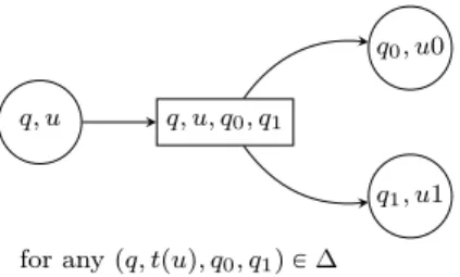
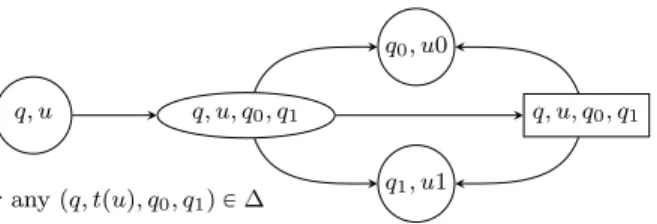
q, u q, u, q0, q1
q0, u0
q1, u1
for any pq, tpuq, q0, q1q P ∆
Figure 1: Local structure of the arena of the acceptance game GA,t.
Fix an automaton A “ xA, Q, qini, ∆, Accy and a tree t and define an acceptance game GA,t, i.e. a game where Éloïse wins if and only if there exists an accepting run of A on t, as follows.
Intuitively, a play in GA,t consists in moving a pebble along a branch of t in a top-down manner: to the pebble is attached a state, and in a node u with state q, Éloïse picks a transition pq, tpuq, q0, q1q P ∆, and then Abélard chooses to move down the pebble either to u ¨ 0 (and update the state to q0) or to u ¨ 1 (and update the state to q1).
Formally (see Figure 1 for an illustration4), let G
A,t“ pVEZ VA, Eq with VE“ Q ˆ t0, 1u˚, VA“ tpq, u, q0, q1q | u P t0, 1u˚ and pq, tpuq, q0, q1q P ∆u Ď Q ˆ t0, 1u˚ˆ Q ˆ Q and
E “ tppq, uq, pq, u, q0, q1qq | pq, u, q0, q1q P VAqu Y tppq, u, q0, q1q, pu ¨ x, qxqq | x P t0, 1u and pq, u, q0, q1q P VAqu Then let GA,t“ pGA,t, VE, VAq and extend Col on VEY VAby letting Colppq, uqq “ Colppq, u, q0, q1qq “ Colpqq. Finally define GA,tas the parity game pGA,t, Colq.
The next theorem is well-known (see e.g. [6, 8]) and its proof is obtained by remarking that strategies for Éloïse in GA,tare in bijection with runs of A on t (with the winning strategies corresponding to the accepting runs).
Theorem 2. One has t P LpAq if and only if Éloïse wins in GA,t from pqini, εq.
3. Automata with Cardinality Constraints and Automata with Topological Bigness Constraints We now introduce the main notions studied in the paper, namely automata with cardinality constraints (studied in Section 4 and Section 5) and automata with topological bigness constraints (studied in Section 6). 3.1. Automata with Cardinality Constraints
We now relax the criterion for a run to be accepting. Recall that classically, a run is accepting if every branch in it is accepting. For a given automaton A, we define the following four criteria (two for the case where one counts the number of accepting branches and two for the case where one counts the number of rejecting branches) for a run to be accepting. Note that the case where one counts accepting branches was already considered in [10, 11].
• There are finitely many rejecting branches in the run. A tree t is in LRejFinpAq if and only if there is a run of A on t satisfying the previous condition.
• There are at most countably many rejecting branches in the run. A tree t is in LRejďCountpAq if and only if there is a run of A on t satisfying the previous condition.
• There are infinitely many accepting branches in the run. A tree t is in LAcc
8 pAq if and only if there is a run of A on t satisfying the previous condition.
• There are uncountably many accepting branches in the run. A tree t is in LAcc
U ncountpAq if and only if there is a run of A on t satisfying the previous condition.
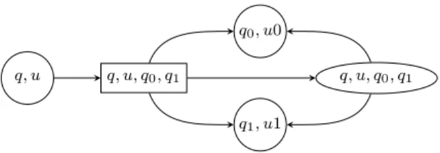
q, u q, u, q0, q1
q0, u0
q1, u1
q, u, q0, q1
for any pq, tpuq, q0, q1q P ∆
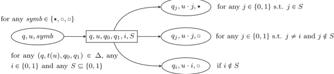
Figure 2: Local structure of GRejďCountA,t .
3.2. Automata with Topological Bigness Constraints
A notion of topological “bigness” and “smallness” is given by large and meager sets respectively (see [19, 20] for a survey of the notion). The idea is to see the set of branches in a tree as a topological space by taking as basic open sets the cones. For a node u P t0, 1u˚, the cone Conepuq is defined as tπ P t0, 1uω
| u Ď πu. A set of branches B Ď t0, 1uω is nowhere dense if for all nodes u, there exists v P t0, 1u˚ such that no branch of B has uv as a prefix. It is meagre if it is the countable union of nowhere dense sets. Finally it is large if it is the complement of a meagre set.
For a given automaton A, we define the following acceptance criterion: a run is accepting if and only if its set of accepting branches is large. Note that this is equivalent to require that the set of rejecting branches is meagre.
Finally, a tree t is in LAcc
LargepAq if and only if there is a run of A on t satisfying the previous condition.
4. Counting Rejecting Branches
For the classes of automata where acceptance is defined by a constraint on the number of rejecting branches we show that the associated languages are ω-regular. For this, we adopt the following roadmap: first we design an acceptance game and then we note that it can be transformed into another equivalent game that turns out to be the (usual) acceptance game for some tree automaton.
Fix, for this section, a parity tree automaton A “ xA, Q, qini, ∆, Coly and recall that a tree t is in LRejďCountpAq (resp. in LRejFinpAq) if and only if there is a run of A on t in which there are at most countably (resp. finitely) many rejecting branches.
4.1. The Case of Languages LRejďCountpAq
Fix a tree t and define an acceptance game for LRejďCountpAq as follows. In this game the two players move a pebble along a branch of t in a top-down manner: to the pebble is attached a state whose colour gives the colour of the configuration. Hence, (Éloïse’s main) configurations in the game are elements of Q ˆ t0, 1u˚. See Figure 2 for the local structure of the arena. In a node u with state q Éloïse picks a transition pq, tpuq, q0, q1q P ∆, and then Abélard has two possible options:
(i) he chooses a direction 0 or 1; or (ii) he lets Éloïse choose a direction 0 or 1.
Once the direction i P t0, 1u is chosen, the pebble is moved down to u ¨ i and the state is updated to qi. A play is won by Éloïse if one of the following two situations occurs: either the parity condition is satisfied or Abélard has not let Éloïse infinitely often choose the direction. Call this game GRejďCountA,t .
The next theorem states that it is an acceptance game for the language LRejďCountpAq. Theorem 3. One has t P LRejďCountpAq if and only if Éloïse wins in GRejďCountA,t from pqini, εq.
Proof. Assume that Éloïse has a winning strategy ϕ in GRejďCountA,t from pqini, εq. With ϕ we associate a run ρ of A on t as follows. We inductively associate with any node u a partial play λu where Éloïse respects ϕ and that ends in a vertex of Éloïse of the form pq, uq. For this we let λε “ pqini, εq. Now assume that we have
defined λu for some node u and let ϕpλuq “pq, tpuq, q0, q1q be the transition Éloïse plays from λu when she respects ϕ. Then let i be the direction Éloïse would choose (again playing according to ϕ) if Abélard lets her pick the direction right after she played pq, tpuq, q0, q1q: one defines λui as the partial play obtained by extending λuby Éloïse choosing transition pq, tpuq, q0, q1q, followed by Abélard letting her choose the direction and Éloïse choosing direction i; and one defines λup1´iqas the partial play obtained by extending λuby Éloïse choosing transition pq, tpuq, q0, q1q, followed by Abélard choosing direction p1 ´ iq. Note that for j P t0, 1u, λuj ends with the pebble on uj with the state qj attached to it, equivalently in configuration pqj, ujq. We also refer to the node ui (i.e. the node that Éloïse has picked) as marked : note that any node has exactly one child that is marked (by convention the root is marked).
The run ρ is defined by letting ρpuq be the state attached to the pebble in the last configuration of λu. By construction, ρ is a valid run of A on t and moreover with any branch π in ρ one can associate a play λπ in GRejďCountA,t from pqini, εq where Éloïse respects ϕ (one simply considers the limit of the increasing sequence of partial plays λu where u ranges over those nodes along branch π).
It remains to show that the number of rejecting branches is at most countable. Now consider a rejecting branch π. By construction π is rejecting if and only if λπdoes not fulfil the parity condition. As ϕ is winning
so does λπ hence, it means that in λπ Abélard does not let Éloïse choose infinitely often the direction (indeed,
this is the only way for λπ to be winning as we assumed π is rejecting, which implies that λπ does not satisfy
the parity condition). Equivalently, π contains finitely many marked nodes (marked nodes corresponding precisely to those steps where Éloïse chooses the direction). Hence, with any rejecting branch π, one can associate the last marked node uπ in it. And if π ‰ π1 one has uπ‰ uπ1: indeed, at the point where π and π1 first differ, one of the node is marked from the property that every node has exactly one child that is marked. Hence, the number of rejecting branches is countable as the map π ÞÑ uπ is injective and as the number of nodes in a tree is countable. This permits to conclude that ρ is an accepting run – in the sense of LRejďCountpAq – of A on t.
Conversely, assume that Éloïse has no winning strategy. It follows from Borel determinacy [21] that Abélard has a winning strategy ψ in GRejďCountA,t from pqini, εq. Let us prove that any run ρ of A on t contains uncountably many rejecting branches. For this, fix a run ρ of A on t. With any sequence α “ α1α2¨ ¨ ¨ P t0, 1uω we associate a strategy ϕαof Éloïse in GRejďCountA,t . The strategy ϕα of Éloïse consists in describing the run ρ and to propose direction αi when it is the i-th time that Abélard lets her choose the direction. More formally, when the pebble is on node u with state q (we will trivially have q “ ρpuq as an invariant) she picks the transition pρpuq, tpuq, ρpu0q, ρpu1qq; moreover if Abélard lets her choose the direction, she picks αi`1 where i is the number of times Abélard let her choose the direction since the beginning of the play.
As we assumed that ψ is winning, the (unique) play obtained when she plays ϕα and when he plays ψ is loosing for Éloïse: such a play defines a branch παin ρ, and this branch is a rejecting one. Now, for any α ‰ α1 one has π
α‰ πα1: indeed, at some point α and α1 differs and, as infinitely often Abélard lets Éloïse choose the directions, the branches πα and πα1 will differ as well. But as there are uncountably many different sequences α, it leads an uncountable number of rejecting branches in ρ. Hence, ρ is rejecting.
Consider the game GRejďCountA,t and modify it so that Éloïse is now announcing in advance which direction she would choose if Abélard let her do so. This new game is equivalent to the previous one (meaning that she has a winning strategy in one game if and only if she also has one in the other game). As this new game can easily be modified to obtain an equivalent acceptance game for the classical acceptance condition (as described in Section 2.3) one concludes that the languages of the form LRejďCountpAq are always ω-regular. Theorem 4. Let A “ xA, Q, qini, ∆, Coly be a parity tree automaton using d colours. Then there exists a parity tree automaton A1 “ xA, Q1, q1
ini, ∆1, Col1y such that L Rej
ďCountpAq “ LpA
1q. Moreover |Q1| “ Opd|Q|q and A1 uses d ` 1 colours.
Proof. Define G1RejďCountA,t as the game obtained from G
RejďCount
A,t by asking Éloïse to say which direction she would choose before Abélard possibly lets her this option. Éloïse has a winning strategy in GRejďCountA,t if and only if she has a winning strategy in G1RejďCountA,t (strategies being essentially the same in both games). The way she indicates the direction can be encoded in the control state: just duplicate the control states (with a classical version and a starred version of each state) and when she wants to pick a transition e.g. pq, tpuq, q0, q1q and direction 1, she just moves to configuration pq, u, q0, q1˚q in the new game. Now the winning
condition can be rephrased as either the parity condition is satisfied or finitely many configuration of the form pq˚, uq are visited. Now this later game can be transformed into a standard acceptance game for ω-regular language (as defined in Section 2.3) by the following trick. One adds to states an integer where one stores the smallest colour seen since the last starred state was visited (this colour is easily updated); whenever a starred state is visited the colour is reset to the colour of the state. Now unstarred states are given an even colour that is greater than all colour previously used (hence, it ensures that if finitely many starred states are visited Éloïse wins) and starred states are given the colour that was stored (hence, if infinitely many starred states are visited we retrieve the previous parity condition). It should then be clear that the later game is a classical acceptance game, showing that LRejďCountpAq is ω-regular.
The construction of A1 is immediate from the final game and the size is linear in d|Q| due to the fact that one needs to compute the smallest colour visited between two starred states.
More formally5, we assume that A uses colours 0, 1, . . . , d ´ 1 and we let A1 “ xA, Q1, q1
ini, ∆1, Col 1 y where: • Q1 “ tq i, qi˚| q P Q and 0 ď i ď d ´ 1u; • q1
ini“ qini,Colpqiniq;
• for any q P Q and any 0 ď i ď d ´ 1 one lets Col1
pqi˚q “ i and Colpqiq “ d ` 1 if d ` 1 is even and
Colpqiq “ d otherwise; and
• ∆1 consists of the following tuples for every pq, a, r, sq P ∆ and every 0 ď i ď d ´ 1
– pqi, a, r˚minti,Colprqu, sminti,Colpsquq,
– pqi, a, rminti,Colprqu, s˚minti,Colpsquq,
– pq˚
i, a, rColprq˚ , sColpsqq, and
– pq˚
i, a, rColprq, s˚Colpsqq.
It is then easily seen that the acceptance game GA1,t of A1 as defined in Section 2.3 is essentially the same as the above game G1RejďCountA,t .
4.2. The Case of Languages LRejFinpAq
The following lemma (whose proof is straightforward) characterises finite sets of branches by noting that for such a set there is a finite number of nodes belonging to at least two branches in the set.
Lemma 1. Let Π be a set of branches. Then Π is finite if and only if the set W “ tu P t0, 1u˚ | Dπ
0‰ π1P Π s.t. u Ď π0 and u Ď π1u is finite. Equivalently, Π is finite if and only if there exists some ` ě 0 such that for all u P t0, 1uě` there is at most one π P Π such that u Ď π.
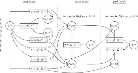
Now, fix a tree t and define an acceptance game for LRejFinpAq as follows. In this game (we refer the reader to Figure 3 for the local structure of the arena for game GRejFinA,t ) the two players move a pebble along a branch of t in a top-down manner: as in the classical case the players first select a transition and then a direction. The colour of the current state gives the colour of the configuration. There are three modes in this game: wait mode, path mode and check mode and the game starts in wait mode. Hence, (Éloïse’s main) configurations in the game are elements of Q ˆ t0, 1u˚ˆ twait, path, checku.
Regardless of the mode, in a node u with state q Éloïse picks a transition pq, tpuq, q0, q1q P ∆, and for each direction in i P t0, 1u she proposes the next mode mi in twait, path, checku (we describe below what are the possible options depending on the current mode). Then Abélard chooses a direction j P t0, 1u, the pebble is moved down to u ¨ j, the state is updated to qj and the mode changes to mj. The possible modes that Éloïse can propose depend on the current mode in the following manner.
• In wait mode she can propose any modes miin twait, path, checku but if one proposed mode mi is path then the other mode m1´i must be check.
5We only give the formal construction of A1for this statement, and will keep it more informal later in similar proofs (namely the ones of theorems 6,8, 11 and 13).
q, u q, u, qw 0, qc1, 0 q, u, qc 0, q w 1, 0 q, u, qw 0, qw1, 0 q, u, qc 0, q p 1, 0 q, u, q0p, qc1, 0 q, u, qc 0, q1c, 0 q0, u0 q1, u1 for an y p q , tp u q , q0 , q1 q P ∆ wait mode q, u q, u, qc 0, q1c, 0 q0, u0 q1, u1
for any pq, tpuq, q0, q1q P ∆
check mode q, u q, u, q0p, qc1, 0 q, u, qc 0, q p 1, 0 q0, u0 q1, u1
for any pq, tpuq, q0, q1q P ∆
path mode
Figure 3: Local structure of the arena of the acceptance game GRejFinA,t . We use superscripts to indicate which modes have been proposed by Éloïse.
• In check mode the proposed modes must be check (i.e. once the mode is check it no longer changes). • In path mode one proposed mode must be path and the other must be check.
A play is won by Éloïse if one of the two following situations occurs. • The wait mode is eventually left and the parity condition is satisfied. • The mode is eventually always equal to path.
In particular a play in which the mode is wait forever is lost by Éloïse. Note that the latter winning condition can easily be reformulated as a parity condition. Call this game GRejFinA,t .
The next theorem states that it is an acceptance game for the language LRejFinpAq. Theorem 5. One has t P LRejFinpAq if and only if Éloïse wins in GRejFinA,t from pqini, ε, waitq.
Proof. Assume that Éloïse has a winning strategy ϕ in GRejFinA,t from pqini, ε, waitq. With ϕ we associate a run ρ of A on t as follows. We inductively define for any node u P t0, 1u˚ a partial play λ
u where Éloïse respects ϕ. For this we let λε“ pqini, ε, waitq. Now assume that we defined λu for some node u P t0, 1u˚ and let pq, tpuq, q0, q1q be the transition Éloïse plays from λu when she respects ϕ. Then for each i P t0, 1u one defines λu¨ias the partial play obtained by extending λuby Éloïse choosing transition pq, tpuq, q0, q1q, followed by Abélard choosing direction i (we update the mode accordingly to the choice of Éloïse when respecting ϕ in λu).
The run ρ is defined by letting, for any u P t0, 1u˚, ρpuq be the state attached to the pebble in the last configuration of λu. By construction, ρ is a run of A on t. Moreover with any branch π one can associate a play λπ in GRejFinA,t from pqini, εq where Éloïse respects ϕ (one simply considers the limit of the increasing sequence of partial plays λu where u ranges over nodes along branch π).
First, note that there exists some ` ě 0 such that, for all u P t0, 1uě`, λ
uends in a vertex where the mode is not wait. Indeed, if this was not the case, one could construct an infinite branch π such that, for all nodes u in π, λu ends with a vertex in mode wait (recall that the only way to be in wait mode is to be in that mode from the very beginning) and therefore the corresponding play λπ would be loosing, which contradicts the fact that Éloïse respects her winning strategy ϕ in play λπ. Now, consider some node u P t0, 1u`. If the final vertex in λu is in mode check one easily verifies that any branch that goes through u is accepting (because the corresponding play is winning hence, satisfies the parity condition). If the final vertex in λuis in mode
path one easily checks that among all branches that go through u, there is exactly one branch π such that λπ eventually stays in mode path forever (and this branch may not satisfy the parity condition) while all other branches eventually stay in mode check forever (and satisfy the parity condition). Therefore, the number of rejecting branches is finite.
Conversely, assume that there is a run ρ of A on t that contains finitely many rejecting branches. Call this set of branches Π. Thanks to Lemma 1, there exists some ` ě 0 such that for all w P t0, 1uě` there is at most one π P Π such that w Ď π. Using ρ we define a strategy ϕ for Éloïse in GRejFinA,t as follows. In any configuration pq, uq (regardless of the mode) the strategy is to play the transition pq, tpuq, ρpu0q, ρpu1qq. Then there are several cases for determining how the mode is updated.
• In some configuration pq, uq with u of length strictly smaller than ` the mode remains in wait.
• In some configuration pq, uq with u of length equal to ` the strategy proposes to update the mode to path for direction i P t0, 1u such that u ¨ i Ď π for some branch π P Π, and to check otherwise. Note that due to the definition of `, there is at most one direction i in which the mode becomes path. • In some configuration pq, uq with u of length strictly greater than ` if the mode is check it will remain
to check in both direction. Otherwise (i.e. the mode is path) the strategy proposes to update the mode to path for direction i P t0, 1u such u ¨ i Ď π for some branch π P Π, and to check otherwise. Note that in the latter case, there is exactly one direction i in which the mode is path.
Remark that no play where Éloïse respects ϕ stays in wait mode forever. Moreover, with any λ where Éloïse respects ϕ one can associate a branch in the run ρ and this branch is rejecting if and only if λ stays eventually in mode path forever. Hence, any play where the mode is not infinitely often path satisfies the parity condition (because the corresponding branch in ρ does so). Hence, ϕ is winning.
From Theorem 5 and the local structure of the arena of game GRejFinA,t one easily concludes that any language of the form LRejFinpAq is ω-regular.
Theorem 6. Let A “ xA, Q, qini, ∆, Coly be a parity tree automaton using d colours. Then, there exists a parity tree automaton A1 “ xA, Q1, q1
ini, ∆1, Col 1
y such that LRejFinpAq “ LpA1q. Moreover, |Q1| “ Op|Q|q and A1 uses d colours.
Proof. Consider the local structure of game GRejFinA,t as described in Figure 3. The way one defines A1 is fairly simple: for any state on A and any mode, one gets a new state in A1, and the transition function ∆1 directly follows from the way we update the modes. The states in wait mode all get the same odd minimal colour (hence, if they are never left Éloïse looses), the states in path mode all get the same even minimal colour (hence, if they are never left Éloïse wins), and the states in check mode get the colour they had in A. Hence, we do not need to add any extra colour (except in the case where A uses only one colour but in this very degenerated case one can simply take A1“ A).
4.3. Languages LRejďCountpAq and LRejFinpAq vs. Büchi Tree Languages
One can wonder, as it will be later the case (see Section 5) for languages of the form LAcc 8 pAq or LAcc
U ncountpAq , whether a Büchi condition is enough to accept (with the classical semantics) a language of the form LRejďCountpAq (resp. LRejFinpAq). The next Proposition answers negatively.
Proposition 1. There is a co-Büchi deterministic tree automaton A such that for any Büchi tree automaton A1, LRej
ďCountpAq ‰ LpA 1
q and LRejFinpAq ‰ LpA1q.
Proof. We choose for A the same automaton that was used by Rabin in [2] to derive a similar statement where one replaces LRejďCountpAq by LpAq and we generalise the proof of this result as given in [4, Example 6.3].
Let L be the set of ta, bu-labelled trees such that the number of branches that contain infinitely many b’s is at most countable. Obviously there is a deterministic co-Büchi automaton A such that L “ LRejďCountpAq. Indeed, consider an automaton A with two states, one forbidden and the other one non-forbidden, and that from any state, goes (for both children) in the forbidden state whenever he was in a b-labelled node and otherwise goes (for both children) in the non-forbidden state.
Assume, by contradiction, that there is some Büchi tree automaton A1
“ xta, bu, Q, qini, ∆, F y such that LRejďCountpAq “ LpA1q. Note that we will not treat the case where LRejFinpAq “ LpA1q as it is identical. Let n “ |Q| and let t be the ta, bu-labelled tree such that tpuq “ b if and only if u P p0`1qk for some 1 ď k ď n, i.e. label b occurs when a right successor is taken after a sequence of left successors, however allowing at most n right turns. Clearly, t P L as every branch contains finitely many b-labelled nodes. Let ρ be an accepting run of A1 on t.
The goal is to exhibit three nodes u, v and w such that: 1. u is a strict prefix of both v and w.
2. v is not a prefix of w and vice versa; 3. ρpuq “ ρpvq “ ρpwq is a final state; 4. tpuq “ tpvq “ tpwq “ a;
5. on the path segment from u to v there is at least one node labelled b; 6. on the path segment from u to w there is at least one node labelled b.
Once this is done we can form a new tree t1 (and an associated run ρ1 of A1 on t1) by iterating the finite path segment from u (inclusive) to v (exclusive) and from u (inclusive) to w (exclusive) indefinitely, copying also the subtrees which have their roots on these path segments. More formally, consider the two-hole context Ctr‚, ‚s (resp. Cρr‚, ‚s) obtained by placing holes at v and w in t (resp. in ρ) and the two-hole context Dtr‚, ‚s (resp. Dρr‚, ‚s) obtained by placing holes at u´1v and u´1w in the subtree t{uof t rooted at u (resp. ρ{u) . The tree t1 is equal to C
trt2, t2s where t2 is the unique tree satisfying the equation t2“ Dtrt2, t2s. Similarly ρ1 is equal to C
ρrρ2, ρ2s where ρ2 is the unique tree satisfying the equation ρ2“ Dρrρ2, ρ2s.
This process exhibits a binary tree like structure6 inside t1 (resp. ρ1) such that any branch in t1 contains infinitely many b-labelled nodes, hence t1 R L (indeed, there will be uncountably many branches in this binary tree like structure). But this leads to a contradiction as ρ1 is easily seen to be accepting while being a run on t1.
We now explain why we can find nodes u, v and w as above. We first claim that for any node u P 0`p10`qk, for some 0 ď k ă n, there are two nodes vu, wuP u0`10` such that (i) u is a strict prefix of vu and wu; (ii) vuis not a prefix of wu and vice versa; and (iii) ρpvuq “ ρpwuq is a final state. Indeed, for any i ą 0, the branch u0i10ωis accepting in ρ and therefore there exists some index k
ią 0 such that ρpu0i10kiq P F ; thus, by the pigeon hole principle, there exists i ‰ j such that ρpu0i10kiq “ ρpu0j10kjq P F and therefore one can choose vu“ u0i10ki and wu“ u0j10kj.
Now define a sequence of nodes u0 Ă u1 Ă u2 Ă ¨ ¨ ¨ Ă un as follows: we let u0 P 0` to be such that ρpu0q P F (such a node exists as the branch 0ω is accepting in ρ); and for all 1 ď i ď n, ui “ vui´1. In particular, one has ρpuiq P F for all 0 ď i ď n and therefore, by the pigeon hole principle there exists 0 ď i ă j ď n such that ρpuiq “ ρpujq. Now, to finish our construction, we simply let u “ ui, v “ uj and w “ wuj´1. This concludes the proof.
5. Counting Accepting Branches
We now consider the case where acceptance is defined by a constraint on the number of accepting branches and we show that the associated languages are ω-regular. It leads to new proofs, that rely on games rather than on logic, of the results in [11].
Fix, for this section, a parity tree automaton A “ xA, Q, qini, ∆, Coly and recall that a tree t is in LAcc8 pAq (resp. LAccU ncountpAq) if and only if there is a run of A on t that contains infinitely (resp. uncountably) many accepting branches.
5.1. The Case of Languages LAcc
8 pAq
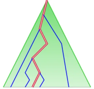
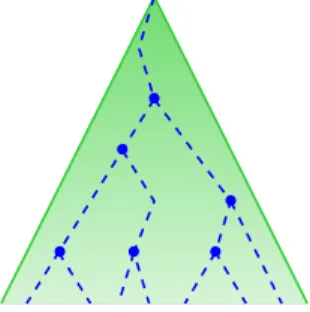
The key idea behind defining an acceptance game for LAcc8 pAq for some tree t is to exhibit a pseudo comb in a run of A over t. In a nutshell, a pseudo comb consists of an infinite branch U and a collection V of accepting branches each of them sharing some prefix with U . One easily proves that a run contains infinitely many accepting branches if and only if it contains a pseudo comb.
Figure 4: A pseudo comb pU,Vq
More formally, a pseudo comb (see Figure 4 for an illustration) is a pair of subset pU, V q of nodes with U, V Ď t0, 1u˚ such that:
• U and V are disjoint.
• U is a branch: ε P U , for all u P U one has |tu0, u1u X U | “ 1and if u ‰ ε its parent is in U as well. • V is a set of nodes such that
(i) for all v P V , one has |tv0, v1u X V | “ 1; (ii) for all v P V , v P pU Y V q ¨ t0, 1u.
• For infinitely many u P U there exists some v P V such that either v “ u0 or v “ u1.
The following folklore lemma characterises infinite sets of branches in the full binary tree (recall that we say that a node w belongs to a branch π if and only if w Ă π).
Lemma 2. Let Π be a set of branches. Then Π is infinite if and only if the set W “ tw | Dπ P Π s.t. w belongs to πu contains a pseudo comb pU, V q, i.e. U Y V Ď W .
Proof. If W contains a pseudo comb it directly implies that Π is infinite, so we focus on the other implication. There exists an increasing sequence (for the prefix relation Ď) puiqiě0 of nodes such that for all i ě 0
infinitely many branches in Π go through ui and for both directions j “ 0 and j “ 1, at least one branch in Π
goes through ui¨ j. The existence of this sequence is by an immediate induction.
Define U as the set of prefixes of elements in the sequence puiqiě0: U is a branch as the sequence puiqiě0 is increasing.
For all i, pick a branch Vi that goes through ui but not through ui`1 (it exists by definition of ui). Then to obtain a pseudo comb pU, V q such that U Y V Ď W , it suffices to define V “ pŤiě0ViqzU .
Now, fix a tree t and define an acceptance game for LAcc
8 pAq. There are two modes in the game (See Figure 5 for the local structure of the arena): path mode and check mode and the game starts in path mode. Hence, (Éloïse’s) configurations in the game are elements of Q ˆ t0, 1u˚ˆ tpath, checku. In path mode, in a node u with state q Éloïse picks a transition pq, tpuq, q0, q1q P ∆, and she chooses a direction i P t0, 1u. Then Éloïse has two options. Either she moves down the pebble to u ¨ i and updates the state to be qi. Or she proposes Abélard to change to check mode: if he accepts, the pebble is moved down to u ¨ p1 ´ iq and the state is updated to qp1´iq; if he refuses, the pebble is moved down to u ¨ i and the state is updated to qi (and the game stays in path mode).
In check mode Éloïse plays alone: in a node u with state q she picks a transition pq, tpuq, q0, q1q P ∆, and she chooses a direction i P t0, 1u; then the pebble is moved down to u ¨ i and the state is updated to qi. Note that it is not possible to switch from check mode back to path mode.
q, u q, u, q0, q1, 0 q, u, q0, q1, 1 q0, u0 q1, u1 q, u, q0, q1, 0 q, u, q0, q1, 1 q1, u1 q0, u0 q, u q, u, q0, q1, 0
for any pq, tpuq, q0, q1q P ∆
path mode check mode
for any pq, tpuq, q0, q1q P ∆
Figure 5: Local structure of the arena of the acceptance game GAcc 8A,t .
• Eventually the players have switched to check mode and the parity condition is satisfied. • Éloïse proposed infinitely often Abélard to switch the mode but he always refused. Call this game GAcc 8
A,t . Intuitively path mode is used to define the U part of the pseudo-comb pU, V q and each of the branches in V is inspected in check mode. Note that in check mode, Éloïse plays alone and hence only checks the existence of an accepting branch. However, as the automata we consider are assumed to be complete hence, there always exists some run containing this accepting branch.
The next theorem states that it is an acceptance game for the language LAcc 8 pAq. Theorem 7. One has t P LAcc
8 pAq if and only if Éloïse wins in GAcc 8A,t from pqini, ε, pathq.
Proof. Assume that Éloïse has a winning strategy ϕ in GAcc 8A,t from configuration pqini, ε, pathq. With ϕ we associate a run ρ of A on t and a pseudo comb pU, V q as follows. We inductively associate with any node u P U a partial play λu where Éloïse respects ϕ and that is always in path mode; and we inductively associate with any node v P V a partial play λv where Éloïse respects ϕ and where the mode has eventually been switched to check mode. For this we let ε P U and λε“ pqini, ε, pathq. Now assume that we defined λu for some node u P U and let pq, tpuq, q0, q1q be the transition and let i be the direction Éloïse plays from λuwhen she respects ϕ. Then we have two possible situations depending whether, right after playing pq, tpuq, q0, q1q and still respecting ϕ, Éloïse proposes Abélard to switch to check mode.
• If she does so we let u ¨p1´iq belong to V and we define λu¨p1´iqas the partial play obtained by extending λu by Éloïse choosing transition pq, tpuq, q0, q1q and direction i, followed by Éloïse proposing Abélard to switch the mode and Abélard accepting (hence, moving down the pebble in direction p1 ´ iq and attaching state qp1´iqto it). We let u ¨ i belong to U and we define λu¨ias the partial play obtained by extending λu by Éloïse choosing transition pq, tpuq, q0, q1q and direction i, followed by Éloïse proposing Abélard to switch the mode and Abélard refusing (hence, moving down the pebble in direction i and attaching state qi to it).
• If Éloïse does not propose Abélard to switch the mode we do not let u ¨ p1 ´ iq belong to V . And we let u ¨ i belong to U and we define λu¨ias the partial play obtained by extending λu by Éloïse choosing transition pq, tpuq, q0, q1q and direction i, followed by Éloïse not proposing Abélard to switch the mode (hence, moving down the pebble in direction i and attaching state qi to it).
The run ρ is defined by letting, for any w P U Y V , ρpwq be the state attached to the pebble in the last configuration of λw. For those w R U Y V we define ρpwq so that the resulting run is valid, which is always
possible as we only consider complete automata. By construction, ρ is a run of A on t and pU, V q is a pseudo comb. Moreover with any branch π that can be built as an initial sequence of nodes in U followed by an infinite sequence of nodes in V one can associate a play λπ in GAcc 8A,t from pqini, ε, pathq where Éloïse respects ϕ (one simply considers the limit of the increasing sequence of partial plays λv where v ranges those nodes nodes in V along branch π). By construction π is accepting as λπ fulfils the parity condition. Hence, by Lemma 2 we conclude that ρ contains infinitely many accepting branches, meaning that t P LAcc8 pAq.
Conversely, assume that Éloïse does not have a winning strategy in GAcc 8A,t from pqini, ε, pathq. By Borel determinacy, Abélard has a winning strategy ψ in GAcc 8A,t from pqini, ε, pathq. By contradiction, assume that there is a run ρ of A on t that contains infinitely many accepting branches. By Lemma 2, it follows that ρ contains a pseudo comb pU, V q such that any branch that can be built as an initial sequence of nodes in U followed by an infinite sequence of nodes in V is an accepting branch. From ρ and pU, V q we define a strategy ϕ of Éloïse in GAcc 8
A,t from pqini, ε, pathq as follows. Strategy ϕ uses as a memory either a node u P U if the play is in path mode or a node v P V if the play is in check mode; initially the memory is u “ ε. Now assume that the pebble is in some node u P U with state q attached to it (one will inductively check that ρpuq “ q). Then there are two possibilities.
• Both u0 and u1 belong to U YV : the strategy ϕ indicates that Éloïse chooses transition pq, tpuq, ρpu0q, ρpu1qq and direction i where ui P U and proposes Abélard to switch to check mode. Then the memory is updated to u ¨ j where j “ i if the mode is unchanged and j “ 1 ´ i otherwise.
• If u0 (resp. u1) belongs to U but u1 (resp. u0) does not belong to V : strategy ϕ indicates that Éloïse chooses the transition pq, tpuq, ρpu0q, ρpu1qq and chooses the direction 0 (resp. 1) and does not propose Abélard to switch to check mode. Then the memory is updated to u0 (resp. u1).
Now assume that the pebble is in some node v P V with state q attached to it: one will inductively check that ρpvq “ q and that the mode is check. Call i the (unique) direction such that vi belongs to V : then the strategy ϕ indicates that Éloïse chooses transition pq, tpvq, ρpv0q, ρpv1qq and then moves down the pebble to direction vi. In particular, once a node in V is reached, strategy ϕ ensures that the pebble always stays in V for the rest of the play.
Now consider the (unique) play λ where Éloïse respects her strategy ϕ while Abélard respects his strategy ψ. As we assumed ψ to be a winning strategy for Abélard, λ is won by him. Now, as pU, V q is a pseudo comb and by definition of ϕ, it follows that λ only goes through nodes in U Y V , and if λ only goes through nodes in U then Éloïse proposes infinitely often to Abélard to switch to check mode. Hence, as λ is winning for Abélard one concludes that eventually the mode is switched in λ and that the resulting play does not fulfil the parity condition. Now, it is easily seen that with λ one associates a branch π in the run ρ and that this branch can be built as an initial sequence of nodes in U followed by an infinite sequence of nodes in V
(indeed, at some point the mode is switched to check and from that point the play stays in nodes from V forever). Now, by definition of a pseudo comb, it follows that the branch π is accepting in ρ which means that it satisfies the parity condition, and therefore so does λ, which brings a contradiction with the fact that it is won by Abélard.
One can modify GAcc 8A,t so that to obtain an equivalent game that has the form of a classical acceptance game. From this follows the fact that the languages of the form LAcc
8 pAq are indeed ω-regular. As the new game can be seen to be obtained from a Büchi automaton, this also permits to lower the acceptance condition. Theorem 8. Let A “ xA, Q, qini, ∆, Coly be a parity tree automaton using d colours. Then there exists a Büchi tree automaton A1 “ xA, Q1, q1
ini, ∆1, Col 1
y such that LAcc8 pAq “ LpA1q. Moreover |Q1| “ Opd|Q|q. Proof. Start from game GAcc 8A,t and observe that if one duplicates the control states (with a classical version and a starred version of each state) and add a Boolean flag Éloïse can indicate the direction she wants to follow and whether she proposes to switch to check mode: e.g. if she wants to choose transition pq, tpuq, q0, q1q and direction 1 and not change the mode, she just moves to configuration pq, u, q0, q1˚, Kq in the new game; if she wants to choose transition pq, tpuq, q0, q1q and direction 0 and offer Abélard the option to switch to check mode she moves to configuration pq, u, q˚
0, q1, Jq. Now, we allow Abélard to choose any direction but if the corresponding state is not starred then either one goes to a dummy winning configuration for Éloïse if the Boolean was K and otherwise one changes the mode to check. We indicate the check mode in the control
state and we use the same trick to let Éloïse impose the choice of the branch (if Abélard does not follow her choice one ends up in the previous dummy configuration). It should be clear that the resulting game is an equivalent acceptance game when equipped with the following winning condition: Éloïse wins if either the dummy configuration is reached, or infinitely many configuration with Boolean J are visited but the play is always in path mode or the play is eventually in check mode and the parity condition holds. Now, the two first criteria are Büchi criteria while the third one is a priori a parity condition. But as Éloïse plays alone in check mode, she can indicate at some point that the smallest infinitely visited colour will be some (even) integer and that no other smaller colour will latter be visited: hence, if one stores the colour, go to a final state whenever it is visited and to a rejecting state if some smaller colour occurs, then one obtains a Büchi condition. All together (combining the Büchi conditions in the usual way) one obtains an equivalent Büchi classical acceptance game, showing that LRejďCountpAq is ω-regular and accepted by a Büchi automaton.
The construction of A1 is immediate from the final game and the size is linear in d|Q| due to the fact that one needs to remember the smallest colour for the check mode.
5.2. The Case of Languages LAccU ncountpAq
We now discuss the case of languages of the form LAcc
U ncountpAq. For this we start with some key objects (accepting pseudo binary trees and k-pseudo binary trees) that are used to characterise runs with uncountably many accepting branches. Then, we describe two acceptance games: the first one is very simple while the second one is more involved but later permits to lower the acceptance condition to Büchi when showing that the languages LAccU ncountpAq are accepted by tree automata with the classical semantics.
5.2.1. Accepting-Pseudo Binary Tree & k-Pseudo Binary Tree The key idea behind defining an acceptance game for LAcc
U ncountpAq for some tree t is to exhibit an accepting pseudo binary tree in a run of A over t. In a nutshell, an accepting pseudo binary tree is an infinite set U of nodes with a tree-like structure between them and such that any branch that has infinitely many prefixes in U is accepting.
We now formally define accepting-pseudo binary trees and k-pseudo binary trees that characterise those runs that contains uncountably many accepting branches (Lemma 3 and Lemma 4 below).
‚ ‚ ‚ ‚ ‚ ‚
Figure 6: An accepting-pseudo binary tree U: nodes in U are marked by the symbol‚and all blue branches are accepting.
Let A “ xA, Q, qini, ∆, Coly be a parity tree automaton and let ρ be a run of A on some tree t.
An accepting-pseudo binary tree in ρ (see Figure 6 for an illustration) is a subset U Ď t0, 1u˚ of nodes such that
(i) for all u P U there are v, w P U such that v “ u0v1 and w “ u1w1 for some v1 and w1P t0, 1u˚; (ii) for all v, w P U the longest common prefix u of v and w belongs to U ;
(iii) any branch π that goes through infinitely many nodes in U is accepting.
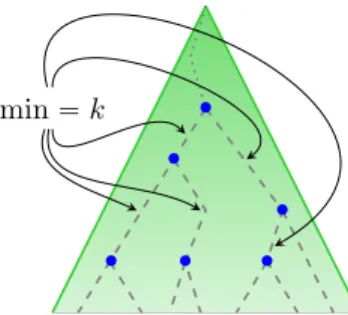
We now give a stronger notion than accepting-pseudo binary tree. For this, let k be some even colour. A k-pseudo binary tree in ρ (see Figure 7 for an illustration) is a subset U Ď t0, 1u˚ of nodes such that
‚ ‚ ‚ ‚ ‚ ‚ min “ k
Figure 7: A k-pseudo binary tree U : nodes in U are marked by symbol‚.
(ii) for all v, w P U the largest common prefix u of v and w belongs to U ; (iii) for all u, v P U such that u Ă v, one has mintColpρpwqq | u Ď w Ď vu “ k.
The following lemma characterises runs that contain an uncountable sets of accepting branches. Its proof is a direct consequence of [11, Lemma 2]. But for the sake of completeness, we give a proof here.
Lemma 3. Let ρ be a run. Then ρ contains uncountably many accepting branches if and only if it contains a k-pseudo binary tree for some even colour k.
Proof. Clearly if ρ contains a k-pseudo binary tree for some even colour k, ρ contains uncountably many accepting branches. It remains to prove the converse.
Let ρ be a run with uncountably many accepting branches. For an even colour k and a node u in ρ, we denote by Πk,u the set of branches π of ρ such that:
• π goes through u (i.e. u Ď π),
• the smallest colour appearing infinitely often in π is k,
• no colour strictly smaller than k appears below u (i.e. for all u Ď v Ď π, ρpvq ě k).
As the set of all accepting branches in ρ is equal to the (countable) union of all the Πk,u, there exists an even colour k0 and a node u0such that Πk0,u0 is uncountable. In the following, we write Π for Πk0,u0.
Claim. For all nodes u Ě u0 such that uncountably many branches of Π go through u, there exists a node wu such that:
• wu is a strict descendant of u (i.e. u Ă wu), • mintColpρpvqq | u Ď v Ď wuu “ k0,
• there are uncountably many branches of Π going though wu0 and through wu1.
If we assume that the claim holds, we can construct a k0-pseudo binary tree by considering the smallest set U such that wu0 belongs to U and such that for all v, v P U implies wv0 P U and wv1P U .
Hence, it remains to show that the claim holds. Let u Ě u0 be a node such that uncountably many branches of Π go through u. Consider the sets:
X :“ tv Ě u | mintColpρpvqq | u Ď w Ď vu “ k0
and uncountably many branches of Π go through v u Y :“ tv Ě u | mintColpρpvqq | u Ď w Ď vu “ k0
and countably many branches of Π go through v u A branch π P Π that goes through u must contain a node in X Y Y . There are two cases:
1. either it contains a node in Y ,
2. or after some position all nodes in π belong to X.
As there are at most countably many branches satisfying Case 1, there must be uncountably many branches satisfying Case 2. In turn this implies that there exists v P X such that both v0 and v1 also belong to X and we can simply take wu to be such a v. Indeed if it was not the case, there would be exactly one branch of Π satisfying Case 2 and going through any given vertex in X: the set of branches satisfying Case 2 would be at most countable.
As any k-pseudo binary tree is an accepting-pseudo binary tree, we directly have the following Lemma from Lemma 3.
Lemma 4. Let ρ be a run. Then ρ contains uncountably many accepting branches if and only if it contains an accepting-pseudo binary tree.
5.2.2. The Acceptance Game GAcc Uncount A,t
q, u q, u, q0, q1
q0, u0
q1, u1
q, u, q0, q1
for any pq, tpuq, q0, q1q P ∆
Figure 8: Local structure of the arena of the acceptance game GAcc Uncount A,t .
Fix a tree t and define an acceptance game for LAccU ncountpAq. In this game (see Figure 8 for the local structure of the arena) the two players move a pebble along a branch of t in a top-down manner: to the pebble is attached a state, and the colour of the state gives the colour of the configuration. Hence, (Éloïse’s main) configurations in the game are elements of Q ˆ t0, 1u˚. In a node u with state q Éloïse picks a transition pq, tpuq, q0, q1q P ∆, and then Éloïse has two options. Either she chooses a direction 0 or 1 or she lets Abélard choose a direction 0 or 1. Once the direction i P t0, 1u is chosen, the pebble is moved down to u ¨ i and the state is updated to qi. A play is won by Éloïse if and only if
(1) the parity condition is satisfied and
(2) Éloïse lets Abélard infinitely often choose the direction during the play. Call this game GAcc UncountA,t .
The next theorem states that it is an acceptance game for the language LAcc
U ncountpAq. Theorem 9. Éloïse wins in GAcc UncountA,t from pqini, εq if and only if t P LAccU ncountpAq.
Proof. In the following proof for a set X Ď t0, 1u˚ we denote by P ref pXq the set of prefixes of elements in X, i.e. PrefpXq “ tu | Dv P X s.t. u Ď vu.
Assume that Éloïse has a winning strategy ϕ in GAcc UncountA,t from pqini, εq. With ϕ we associate a run ρ of A on t and an accepting-pseudo binary tree U as follows. We inductively define U and PrefpU q and associate with any node u P PrefpU q a partial play λu where Éloïse respects ϕ. Remark that even if PrefpU q
is uniquely determined by U we independently define them, making sure that they are indeed compatible. For this we let ε P PrefpU q and we set λε“ pqini, εq.
Now assume that we have defined λu for some node u P PrefpU q. Then let pq, tpuq, q0, q1q be the transition Éloïse plays from λu when she respects ϕ. Then we have two possible situations depending whether, right after playing pq, tpuq, q0, q1q and still respecting ϕ, Éloïse chooses the direction or lets Abélard make that choice. If she chooses the direction, let i be this direction: then one lets ui P PrefpU q and defines λu¨i as the partial play obtained by extending λu by Éloïse choosing transition pq, tpuq, q0, q1q, followed by Éloïse
choosing direction i. If she lets Abélard choose the direction, one lets u belong to U and lets both u0 and u1 belongs to PrefpU q and defines λu¨ifor i P t0, 1u as the partial play obtained by extending λu by Éloïse choosing transition pq, tpuq, q0, q1q, followed by Éloïse letting Abélard choose the direction and Abélard picking direction i. Note that for any ui P PrefpU q, λu¨i ends with the pebble on u ¨ i with state qi attached to it, equivalently in configuration pqi, uiq.
The run ρ is defined by letting, for any u P PrefpU q, ρpuq be the state attached to the pebble in the last configuration of λu. For those u R PrefpU q we define ρpuq so that the resulting run is valid, which is always possible as we only consider complete automata. By construction, ρ is a run of A on t. Moreover, with any branch π consisting only of nodes in PrefpU q, one can associate a play λπ in GAcc UncountA,t from pqini, εq where Éloïse respects ϕ (one simply considers the limit of the increasing sequence of partial plays λu where u ranges over nodes along branch π). As λπ is winning it follows easily that U is a pseudo binary tree (indeed, condition piq and piiq from the definition of an accepting-pseudo binary tree are immediate, while condition piiiq follows from the fact that λπ is winning). Hence, from Lemma 4 we conclude that ρ contains uncountably many accepting branches, meaning that t P LAccU ncountpAq.
Conversely, assume that there is a run ρ of A on t that contains uncountably many accepting branches. By Lemma 4, it follows that ρ contains an accepting-pseudo binary tree U .
From ρ and U we define a strategy ϕ of Éloïse in GAcc Uncount
A,t from pqini, εq as follows. Strategy ϕ uses as a memory a node v P PrefpU q, and initially v “ ε. Now assume that the pebble is on some node v with state q attached to it (one will inductively check that v P PrefpU q and that ρpvq “ q). Then we have two possibilities.
• Assume v P U . Both v0 and v1 belong to PrefpU q: strategy ϕ indicates that Éloïse chooses transition pq, tpvq, ρpv0q, ρpv1qq and let Abélard choose the direction, say i. Then the memory is updated to v ¨ i. • Assume v R U . Hence, v ¨ i belong to PrefpU q for only one i P t0, 1u: strategy ϕ indicates that Éloïse chooses transition pq, tpvq, ρpv0q, ρpv1qq and chooses direction i. Then the memory is updated to v ¨ i. Now consider a play λ where Éloïse respects her strategy ϕ. It is easily seen that with λ one associates a branch π in the run ρ and that this branch goes only through nodes in PrefpU q. From this observation and from the definition of an accepting-pseudo binary tree, we conclude that λ is winning for Éloïse (it satisfies the parity condition as π does and in λ Éloïse lets Abélard choose the direction infinitely often, namely whenever her memory v belongs to U ). Hence, we conclude that strategy ϕ is winning from pqini, εq.
5.2.3. The Acceptance Game rGAcc Uncount A,t One can modify GAcc Uncount
A,t to obtain an equivalent game that has the form of a classical acceptance game. From this follows the fact that the languages of the form LAcc
U ncountpAq are indeed ω-regular. Nevertheless, using a more involved game than GAcc Uncount
A,t one can obtain a stronger result where the acceptance condition is lowered to a Büchi condition. We now describe this game.
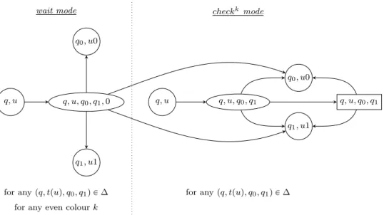
Fix a tree t and define an acceptance game for LAcc
U ncountpAq. There are two modes in the game (See Figure 9 for the local structure of the arena): wait mode and check mode and the game starts in wait mode. Moreover the check mode is parametrised by a colour k. Again, the two players move a pebble along a branch of t in a top-down manner. Hence, (main) configurations in the game are elements of Q ˆ t0, 1u˚ˆ twait, check0, . . . , check2`
u where t0, . . . , 2`u are the even colours used by A. In wait mode Éloïse plays alone: in a node u with state q she picks a transition pq, tpuq, q0, q1q P ∆, and she chooses a direction i P t0, 1u; then the pebble is moved down to u ¨ i and the state is updated to qi. When moving the pebble down she can decide to switch the mode to some checkk (for any even colour k). Once entered checkk mode the play stays in that mode forever and goes as follows. In a node u with state q Éloïse picks a transition pq, tpuq, q0, q1q P ∆, and then she has two possible options. Either she chooses a direction 0 or 1 or she lets Abélard choose a direction 0 or 1. Once the direction i P t0, 1u is chosen, the pebble is moved down to u ¨ i and the state is updated to qi. A play is won by Éloïse if and only if
(1) it eventually enters some checkk mode and
(2) it goes infinitely often through configurations in tpq, u, checkk
q | Colpqq “ ku, (3) it never visits a configuration in tpq, u, checkk
q1, u1 q0, u0
q, u q, u, q0, q1, 0 wait mode
for any pq, tpuq, q0, q1q P ∆ for any even colour k
q, u q, u, q0, q1
q0, u0
q1, u1
q, u, q0, q1
for any pq, tpuq, q0, q1q P ∆ checkkmode
Figure 9: Local structure of the arena of the acceptance game rGAcc UncountA,t .
(4) Éloïse lets Abélard infinitely often choose the direction during the play, and between two such situations the smallest colour visited is always k.
The next theorem states that it is an acceptance game for the language LAccU ncountpAq. Note that its proof is a refinement of the one of Theorem 9.
Theorem 10. One has t P LAcc
U ncountpAq if and only if Éloïse wins in rG
Acc Uncount
A,t from pqini, ε, waitq. Proof. In the following proof for a set X Ď t0, 1u˚ we denote by P ref pXq the set of prefixes of elements in X, i.e. PrefpXq “ tu | Dv P X s.t. u Ď vu.
Assume that Éloïse has a winning strategy ϕ in rGAcc UncountA,t from pqini, ε, waitq. With ϕ we associate a run ρ of A on t and a k-pseudo binary tree U (for some k to be defined later) as follows. We inductively define U and PrefpU q(even if PrefpU q is uniquely determined by U we independently define them, making sure that they are indeed compatible)and associate with any node u P PrefpU q a partial play λuwhere Éloïse respects ϕ. For this we let ε P PrefpU q and we let λε“ pqini, ε, waitq.
Now assume that we have defined λu for some node u P PrefpU q and that the mode in λuis always wait. Then let pq, tpuq, q0, q1q be the transition and let i be the direction Éloïse plays from λu when she respects ϕ. If she does not change the mode, then one lets ui P PrefpU q and defines λu¨ias the partial play obtained by extending λu by Éloïse choosing transition pq, tpuq, q0, q1q, followed by Éloïse choosing direction i and keeping the mode to wait. If she changes the mode to checkk, then one lets ui P PrefpU q and defines λ
u¨ias the partial play obtained by extending λu by Éloïse choosing transition pq, tpuq, q0, q1q, followed by Éloïse choosing direction i and changing the mode to checkk (this k is the one such that U is a k-pseudo binary tree U ).
Now assume that we have defined λufor some node u P PrefpU q and that the mode in λuhas been switched from wait to checkk. Then let pq, tpuq, q
0, q1q be the transition Éloïse plays from λu when she respects ϕ. Then we have two possible situations depending whether, right after playing pq, tpuq, q0, q1q and still respecting ϕ, Éloïse chooses the direction or lets Abélard make that choice. If she chooses the direction, let i be this direction: then one lets ui P PrefpU q and defines λu¨ias the partial play obtained by extending λu by Éloïse choosing transition pq, tpuq, q0, q1q, followed by Éloïse choosing direction i. If she lets Abélard choose the direction, one lets u belongs to U and lets both u0 and u1 belongs to PrefpU q and defines λu¨ifor i P t0, 1u as the partial play obtained by extending λu by Éloïse choosing transition pq, tpuq, q0, q1q, followed by Éloïse letting Abélard choose the direction and Abélard picking direction i. Note that for any ui P PrefpU q, λu¨i ends with the pebble on u ¨ i with state qi attached to it, equivalently in configuration pqi, uiq.
The run ρ is defined by letting, for any u P PrefpU q, ρpuq be the state attached to the pebble in the last configuration of λu. For those u R PrefpU q we define ρpuq so that the resulting run is valid, which is always