Validating object-oriented design metrics on a commercial Java application

Publisher’s version / Version de l'éditeur:

Vous avez des questions? Nous pouvons vous aider. Pour communiquer directement avec un auteur, consultez la

première page de la revue dans laquelle son article a été publié afin de trouver ses coordonnées. Si vous n’arrivez pas à les repérer, communiquez avec nous à [email protected].

Questions? Contact the NRC Publications Archive team at

[email protected]. If you wish to email the authors directly, please see the first page of the publication for their contact information.

https://publications-cnrc.canada.ca/fra/droits

L’accès à ce site Web et l’utilisation de son contenu sont assujettis aux conditions présentées dans le site LISEZ CES CONDITIONS ATTENTIVEMENT AVANT D’UTILISER CE SITE WEB.

Report (National Research Council of Canada. Radio and Electrical Engineering

Division : ERB), 2000

READ THESE TERMS AND CONDITIONS CAREFULLY BEFORE USING THIS WEBSITE.

https://nrc-publications.canada.ca/eng/copyright

NRC Publications Archive Record / Notice des Archives des publications du CNRC :

https://nrc-publications.canada.ca/eng/view/object/?id=c83b709c-c496-4783-b680-13b44c12b44d https://publications-cnrc.canada.ca/fra/voir/objet/?id=c83b709c-c496-4783-b680-13b44c12b44d

NRC Publications Archive

Archives des publications du CNRC

For the publisher’s version, please access the DOI link below./ Pour consulter la version de l’éditeur, utilisez le lien DOI ci-dessous.

https://doi.org/10.4224/8914217

Access and use of this website and the material on it are subject to the Terms and Conditions set forth at

Validating object-oriented design metrics on a commercial Java

application

National Research Council Canada Institute for Information Technology Conseil national de recherches Canada Institut de technologie de l'information

Validating Object-Oriented Design Metrics on a

Commercial Java Application *

Glasberg, D., El-Emam, K., Memo, W., Madhavji, N.

September 2000

* published as NRC/ERB-1080. September 2000. 54 pages. NRC 44146.

Copyright 2000 by

National Research Council of Canada

Permission is granted to quote short excerpts and to reproduce figures and tables from this report, provided that the source of such material is fully acknowledged.

National Research Council Canada Institute for Information Technology Conseil national de recherches Canada Institut de Technologie de l’information

Validating Object-oriented

Design M etrics on a

Commercial Java Application

Daniela Glasberg, Khaled El Emam,

Walcelio Melo, and Nazim Madhavji

September 2000

Validating Object-Oriented

Design Metrics on a Commercial

Java Application

Daniela Glasberg1 Khaled El Emam2 Walcelio Melo3 Nazim Madhavji4

Abstract

Many of the object-oriented metrics that have been developed by the research community are believed to measure some aspect of complexity. As such, they can serve as leading indicators of problematic classes, for example, those classes that are most fault-prone. If faulty classes can be detected early in the development project’s life cycle, mitigating actions can be taken, such as focused inspections. Prediction models using design metrics can be used to identify faulty classes early on. In this paper, we present a cognitive theory of object-oriented metrics and an empirical study which has as objectives to formally test this theory while validating the metrics and to build a post-release fault–proneness prediction model. The cognitive mechanisms which we apply in this study to object-oriented metrics are based on contemporary models of human memory. They are: familiarity, interference, and fan effects. Our empirical study was performed with data from a commercial Java application. We found that Depth of Inheritance Tree (DIT) is a good measure of familiarity and, as predicted, has a quadratic relationship with fault–proneness. Our hypotheses were confirmed for Import Coupling to other classes, Export Coupling and Number of Children metrics. The Ancestor based Import Coupling metrics were not associated with fault-proneness after controlling for the confounding effect of DIT. The prediction model constructed had a good accuracy. Finally, we formulated a cost savings model and applied it to our predictive model. This demonstrated a 42% reduction in post-release costs if the prediction model is used to identify the classes that should be inspected.

1 Introduction

A considerable number of object-oriented metrics have been developed by the research community. The basic premise behind these metrics is that they capture some elements of object-oriented software complexity. Examples of metrics include those defined in (Abreu and Carapuca, 1994; Benlarbi and Melo, 1999; Briand et al., 1997; Cartwright and Shepperd, 2000; Chidamber and Kemerer, 1994; Henderson-Sellers, 1996; Li and Henry, 1993; Lorenz and Kidd, 1994; Tang et al., 1999). While many of these metrics are based on seemingly good ideas about what is important to measure in object-oriented software to capture its complexity, it is still necessary to empirically validate them.

1

School of Computer Science McGill University, 3480 University Street, McConnell Engineering Building, Montreal, Quebec, Canada H3A 2A7. [email protected]

2

National Research Council of Canada, Institute for Information Technology, Building M-50, Montreal Road, Ottawa, Ontario, Canada K1A OR6. [email protected]

3

Oracle Brazil, SCN Qd. 2 Bl. A, Ed. Corporate, S. 604, 70712-900 Brasilia, DF, Brazil. [email protected]

4

School of Computer Science McGill University, 3480 University Street, McConnell Engineering Building, Montreal, Quebec, Canada H3A 2A7. [email protected]

Empirical validation involves demonstrating an association between the metric under study and other measures of important external attributes (ISO/IEC-14598-1, 1996). An external attribute is concerned with how the product relates to its environment (Fenton, 1991). Examples of external attributes are testability, reliability and maintainability. Practitioners, whether they are developers, managers, or quality assurance personnel, are really concerned with the external attributes. However, they cannot measure many of the external attributes directly until quite late in a project’s or even a product’s life cycle. Therefore, they can use product metrics as leading indicators of the external attributes that are important to them. By having good leading indicators, it is possible to predict the external attributes and take early action if the predictions do not fit a project’s objectives. For instance, if we know that a certain coupling metric is a good leading indicator of maintainability as measured in terms of the effort to make a corrective change, then we can minimize coupling during design because we know that in doing so we are also increasing maintainability.

In this paper we focus on empirically validating a set of object-oriented design metrics developed by Chidamber and Kemerer (Chidamber and Kemerer, 1994) and Briand et al. (Briand et al., 1997). The study was performed with data collected from a commercial Java application that implements an XML editor. The external attribute that we measure for our study is reliability. Reliability can be measured in different ways. We measure it in terms of the incidence of a post-release fault in a class. This is termed the fault-proneness of a class.

While previous empirical validation studies of these metrics have been performed (Briand et al., 1997; Briand et al., 1998a; Briand et al., 2000; El-Emam et al., 1999, 2000b; El-Emam et al., 2001b), our current work is intended to replicate these studies in order to provide accumulating evidence of the metrics’ validity. Furthermore, we make a number of additional contributions to the above studies:

• We present a detailed cognitive theory to justify the above metrics. Based on this theory we

state a number of precise hypotheses relating the design metrics to fault-proneness. Evidence supporting the hypotheses suggests possible reasons why certain metrics are leading indicators of fault-proneness. To our knowledge, this is the first attempt at postulating a detailed cognitive theory for object-oriented metrics.

• An object-oriented metrics cost-benefit model is formulated. This model can be used to

evaluate the cost savings from using the design metrics to predict which classes are most fault-prone, and target these classes for inspection. The model is then applied to illustrate its utility.

Our results indicate that many of the design metrics are indeed associated with fault-proneness. The directions of the associations conform to what we predicted from the cognitive theory. This is encouraging as now we have evidence for some cognitive mechanisms to explain the impact of object-oriented metrics. We also built a fault-proneness prediction model using a subset of the validated metrics. The fault-proneness prediction model was found to have high accuracy, and the post-release cost savings from the application of the prediction model were estimated to be 42%. This means that had the prediction model been used to identify the classes to inspect (i.e., those with the highest predicted fault-proneness), then 42% of the post-release costs (i.e., costs associated with dealing with faults discovered by customers) would have been saved. For many organizations such savings are nontrivial, and can free up resources to add features to their products.

In the next section we present a theory that provides mechanisms explaining why the object-oriented metrics we study would be associated with fault-proneness, and give an overview of the metrics we study. Section 3 presents our research method in detail, and our results are presented and discussed in Section 4. We conclude the paper in Section 5 with a summary and directions for future work.

2 Background

Below we present a detailed cognitive theory of object-oriented metrics. The theory explains the mechanisms as to why object-oriented metrics are associated with fault-proneness. By giving the mechanisms, it predicts which metrics are likely to be associated with class fault-proneness, and the direction and functional form of the association. In our study we then empirically test these predictions.

It is important to articulate this theory in detail so that it can be tested. If the theory can be supported empirically, then it is possible to devise better metrics (i.e., with greater predictive power or that can be collected early in the life cycle). Furthermore, if we understood the mechanism then it is plausible that we can improve the design and programming process to avoid the introduction of faults altogether. It is also possible that hypotheses derived from a cognitive theory cannot be empirically supported. In such a case cognitive complexity may not be the reason why certain structural properties of object-oriented applications are problematic, and we have to focus our attention on finding the mechanism of fault introduction.

2.1 Overview of the Cognitive Theory

In order for object-oriented metrics to be associated with fault-proneness, there has to be a mechanism causing this effect. In the software engineering literature, this mechanism is believed to be cognitive complexity. For instance, Munson and Khoshgoftaar (Munson and Khoshgoftaar, 1992) state that “There is a clear intuitive basis for believing that complex programs have more faults in them than simple programs”. It has been argued that a detailed cognitive model is a necessary basis for developing software product metrics (Bergantz and Hassell, 1991; Ehrlich and Soloway, 1984). A further argument has been made that unless there is an understanding of the cognitive demands that software places on developers, then only surface features of the software will be measured, and such surface “complexity” features will not be effective (Sebrechts and Black, 1982). This implies that a cognitive theory of object-oriented metrics that explains how and why certain metrics are associated with fault-proneness is necessary.

Figure 1 depicts the cognitive theory that we describe. The rationale for the theory is the common belief that the structural properties of a software component (such as its coupling and inheritance relationships) have an impact on its cognitive complexity (Briand et al., 2000; Cant et al., 1994; Cant et al., 1995; Henderson-Sellers, 1996).

Structural Class Properties

Comprehension External Attributes (e.g., reliability)

affect

affect

Recall

OO Metrics Pr(Fault)

Figure 1: Overview of object-oriented metrics theory. The dotted lines indicate a relationship

between specific metrics and the concepts that they are measuring. The dashed line depicts the relationship that is actually tested in validation studies. The filled lines indicate hypothesized relationships that explain why structural class properties are associated with external attributes.

One way to operationalize cognitive complexity is to equate it with the ease of comprehending an object-oriented application. If classes are difficult to comprehend then there is a greater probability that faults will be introduced during development. For example, modifications due to requirements changes or fixing faults found during inspections and testing will be error-prone. Furthermore, it will be more difficult to detect faults during the development fault detection activities, such as inspections. In both cases there is a positive association between comprehension and reliability.

A number of studies indicate that certain features of object-oriented application impede their comprehension. Widenbeck et al. (Wiedenbeck et al., 1999) make a distinction between program functionality at the local level and at the global (application) level. At the local level they argue that the object-oriented paradigm’s concept of encapsulation ensures that methods are bundled together with the data on which they operate, making it easier to construct appropriate mental models and specifically to understand a class’ individual functionality. At the global level, functionality is dispersed among many interacting classes, making it harder to understand what the program is doing. They support this in an experiment where they found that the number of correct answers for subjects comprehending a C++ program (with inheritance) on questions about its functionality was not much better than guessing. In another experimental study with students and professional programmers (Boehm-Davis et al., 1992), Boehm-Davis et al. compared maintenance time for three pairs of functionally equivalent programs (implementing three different applications amounting to a total of nine programs). Three programs were implemented in a straight serial structure (i.e., one main function, or monolithic program), three were implemented following the principles of functional decomposition, and three were implemented in the object-oriented style, but without inheritance. In general, it took the students

more time to change the object-oriented programs, and the professionals exhibited the same effect, although not as strongly. Furthermore, both the students and professionals noted that they found that it was most difficult to recognize program units in the object-oriented programs, and the students felt that it was also most difficult to find information in the object-oriented programs. Typically, structural properties that capture dependencies among classes are believed to exert significant influence on comprehension, for example, coupling and inheritance. Coupling metrics

characterize the static5 usage dependencies among the classes in an object-oriented system

(Briand et al., 1999a). Inheritance is also believed to play an important role in the complexity of object-oriented applications. Coupling and inheritance capture dependencies among the classes. Below we present evidence indicating that there is typically a profusion of dependencies in object-oriented applications, and that these dependencies have an impact on understandability and fault-proneness.

The object-oriented strategies of limiting a class’ responsibility and reusing it in multiple contexts results in a profusion of small classes in object-oriented systems (Wilde et al., 1993). For instance, Chidamber and Kemerer (Chidamber and Kemerer, 1994) found in two systems

studied6 that most classes tended to have a small number of methods (0-10), suggesting that

most classes are relatively simple in their construction, providing specific abstraction and

functionality. Another study of three systems performed at Bellcore7 found that half or more of

the methods are fewer than four Smalltalk lines or two C++ statements, suggesting that the classes consist of small methods (Wilde et al., 1993). Many small classes imply many interactions among the classes and a distribution of functionality across them.

It has been stated that “Inheritance gives rise to distributed class descriptions. That is, the complete description for a class D can only be assembled by examining D as well as each of D’s superclasses. Because different classes are described at different places in the source code of a program (often spread across several different files), there is no single place a programmer can turn to get a complete description of a class” (Leijter et al., 1992). While this argument is stated in terms of source code, it is not difficult to generalize it to design documents.

Cant et al. (Cant et al., 1994) performed an empirical study whereby they compared subjective ratings by two expert programmers of the complexity of understanding classes with objective measures of dependencies in an object-oriented system. Their results demonstrate a correlation between the objective measures of dependency and the subjective ratings of understandability. In an experience report on learning and using Smalltalk (Nielsen and Richards, 1989), the authors found that the distributed nature of the code causes problems when attempting to understand a system.

Dependencies also make it more difficult to detect faults. For example, Dunsmore et al. (Dunsmore et al., 2000) note that dependencies in object-oriented programs lead to functionality being distributed across many classes. The authors performed a study with student subjects where the subjects were required to inspect a Java program. The results indicated that the most difficult faults to find were those characterized by a delocalization of information needed to fully understand the fault. A subsequent survey of experienced object-oriented professionals indicated that delocalization was perceived to be a major problem in terms of fault introduction and understandability of object-oriented applications.

We postulate that the extent of dependencies has an impact on comprehension. In Figure 1 we show the constructs of this theory. There are four constructs: (i) structural class properties, (ii) recall, (iii) comprehension, and (iv) external attributes. In software engineering work, we only measure the first and fourth constructs. So we have object-oriented metrics to measure

5

Here static means without the actual execution of the application.

6

One system was developed in C++, and the other in Smalltalk.

7

The study consisted of analyzing C++ and Smalltalk systems and interviewing the developers for two of them. For a C++ system, method size was measured as the number of executable statements, and for Smalltalk size was measured by uncommented nonblank lines of code.

dependencies among classes, and we have metrics of the incidence of faults to measure reliability. We expect that these two will be related. The reason that they are related is explained by the relations through recall and comprehension. In the appendix (Section 8) we elaborate on the theory in detail, presenting the evidence supporting its formulation.

Research on procedural and object-oriented program comprehension has identified three types of mental models that developers construct and update during comprehension (von Mayrhauser and Vans, 1995a). Developers will frequently switch their attention among these mental models. However, during comprehension it is necessary to search and extract information from the program being comprehended, and to connect information within each of these mental models. This requires the recall of information already extracted to construct the mental models.

Dependencies in an object-oriented artifact make it difficult for someone to recall information about the artifact. This impedes comprehension and results in incomplete mental models. Some commonly known effects in cognitive psychology to explain this are: interference effects, fan

effects, and familiarity.

Interference effects occur when a subject learns intervening material after some initial material. The initial material will be more difficult to recall. Fan effects occur when a concept that has been learned has many other concepts associated with it. This leads to that concept being difficult to recall. Familiarity occurs when a concept in memory is repeatedly recalled, and so it becomes easier to recall again.

Based on studies of engineers comprehending an object-oriented system (Burkhardt et al., 1998), we postulate that the way they trace through the class hierarchy when trying to understand the relationship among classes can be mapped to the cognitive effects above. For example, when an engineer is trying to comprehend a class X and encounters an attribute whose type is another class Y, then s/he will proceed to class Y to comprehend what it is doing. This results in an interference effect while comprehending class X. The more class X has connections to other classes, the more difficult it will be to recall information about X due to the fan effect. Furthermore, if class X is an attribute in many other classes, then it will be consulted often during comprehension and therefore will be familiar.

For general recall task as well as for program recall, it has been found that recall is associated with comprehension. The lack of comprehension leads to the introduction of faults, and a difficulty in finding faults during defect detection activities.

It should be noted that this theory is not intended to define all the mechanisms that are believed or that have been shown in the past to have an impact on fault-proneness. But rather, we wish to only focus on the factors that can plausibly explain the relationship between structural class properties and reliability. The limitations of this theory are further elaborated in Section 4.10.

2.2 Structural Class Properties and Their Measurement

Different sets of metrics have been developed in software engineering to capture these object-oriented dependencies. We will focus here on metrics that characterize the inheritance hierarchy and coupling among classes.

The metrics used in our study are a subset of the two sets of metrics defined by Chidamber and Kemerer (Chidamber and Kemerer, 1994) and Briand et al. (Briand et al., 1997). This subset, consisting of metrics that can be collected during the design stage of a project, includes inheritance and coupling metrics (and excludes cohesion and traditional complexity metrics). They are summarized in Table 1. Details of their computation and an illustrative Java example are given in the Appendix (Section 7).

Metric Acronym

Definition

NOC This is the Number of Children inheritance metric (Chidamber and Kemerer, 1994).

This metric counts the number of classes that inherit from a particular class (i.e., the number of classes in the inheritance tree down from a class).

DIT The Depth of Inheritance Tree (Chidamber and Kemerer, 1994) metric is defined as

the length of the longest path from the class to the root in the inheritance hierarchy.

ACAIC OCAIC DCAEC OCAEC ACMIC OCMIC DCMEC OCMEC

These coupling metrics are counts of interactions among classes. The metrics distinguish among the class relationships (friendship, inheritance, none), different types of interactions, and the locus of impact of the interaction (Briand et al., 1997). The acronyms for the metrics indicate what types of interactions are counted:

• The first or first two letters indicate the relationship:

• A: coupling to ancestor classes;

• D: coupling to descendents; and

• O: other, (i.e., none of the above).

• The next two letters indicate the type of interaction between classes c and d:

• CA: there is a class-attribute interaction between classes c and d if c has an

attribute of type d; and

• CM: there is a class-method interaction between classes c and d if class c

has a method with a parameter of type class d.

• The last two letters indicate the locus of impact:

• IC: Import Coupling; and

• EC: Export Coupling

WMC This is the Weighted Methods per Class metric (Chidamber and Kemerer, 1994), and

can be classified as a traditional complexity metric. It is a count of the methods in a class. It has been suggested that neither methods from ancestor classes nor friends in C++ be counted (Basili et al., 1996; Chidamber and Kemerer, 1995). The developers of this metric leave the weighting scheme as an implementation decision (Chidamber and Kemerer, 1994). Some authors weight it using cyclomatic complexity (Li and Henry, 1993). However, others do not adopt a weighting scheme (Basili et al., 1996; Tang et al., 1999). In general, if cyclomatic complexity is used for weighting then WMC cannot be collected at early design stages. Alternatively, if no weighting scheme is used then WMC becomes simply a size measure (the number of methods implemented in a class), also known as NM.

Table 1: Summary of metrics used in our study. The top set are the coupling and inheritance

metrics. The metric at the bottom is used to measure size.

2.3 Hypotheses

The above brief exposition has presented a cognitive theoretical basis for object-oriented metrics. We also presented the metrics that we are evaluating. Based on this we can state precise hypotheses about the direction and functional form of the association between each of the metrics and fault-proneness. In many instances there are competing theories. Table 2 includes a summary of all the hypotheses that we have formulated. The detailed justification for these hypotheses is presented in the Appendix (Section 8). The empirical study below tests these hypotheses and will allow us to determine which of the competing hypotheses can be supported empirically.

Export Coupling Hypotheses

• H-EC+ : Positive Association Classes with high export coupling have many assumptions

made about their behavior. This makes it easier to violate some of these assumptions. This can be seen as a fan effect. Furthermore, more interference will occur as the engineers trace back frequently from classes with high export coupling to understand how they are used. Given that these mechanisms are in the same direction, it is not possible to disentangle them. We therefore consider them together as one hypothesis.

• H-EC- : Negative Association Classes with high export coupling are more familiar because

they are consulted often. Furthemore, classes with high export coupling are given extra attention during development. Given that these two mechanisms are in the same direction, it is not possible to disentangle them. Therefore, by definition it is not possible in an observational study to determine which one of these two mechanisms is operating. We therefore consider them together as one hypothesis.

Inheritance Hypotheses

• H-NOC0: No Association There is no association between NOC and fault-proneness

because the only effect of NOC will be due to the confounding influence of descendant-based export coupling.

• H-DITQ: Qudratic Association Classes at the root are consulted more often, and therefore

they are more familiar. Classes deeper in the hierarchy are also consulted more often. Classes in the middle of the inheritance hierarchy are, in general, not consulted often and therefore they are not familiar. This suggests a quadratic relation between DIT and fault-proneness.

• H-DIT+: Linear Positive Association Root classes are most familiar, but the hierarchy is

not well constructed, and therefore there exists higher conceptual entropy at the deepest classes. This will result in the root classes having few faults and the deeper classes having the most faults.

Import Coupling Hypotheses

• H-IC+: Positive Association Due to interference and fan effects, there will be a positive

association between import coupling and fault-proneness.

Table 2: Summary of hypotheses relating the object-oriented metrics to fault-proneness.

3 Research Method

In this section we present the methodological details of our empirical study.

3.1 Measurement

3.1.1 Object-Oriented Metrics

The object-oriented design metrics described above were collected using a Java static code analyzer (Farnese et al., 1999). No Java inner classes were considered. In order to validate the metrics, we also need to control for the potential confounding effect of size (El-Emam et al., 2000b). The size measure used was NM (the total number of methods defined in the class).

3.1.2 Fault Measurement

In the context of building quantitative models of software faults, it has been argued that considering faults causing field failures is a more important question to address than faults found during testing (Binkley and Schach, 1998). In fact, it has been argued that it is the ultimate aim of quality modeling to identify post-release fault-proneness (Fenton and Neil, 1999). In at least one

study it was found that pre-release fault-proneness is not a good surrogate measure for post-release fault-proneness, the reason posited being that pre-post-release fault-proneness is a function of testing effort (Fenton and Ohlsson, 2000).

Therefore, faults counted for the system that we studied were due to field failures occuring during actual usage. For each class we characterized it as either faulty or not faulty. A faulty class had at least one fault detected during field operation. Distinct failures that are traced to the same fault are counted as a single fault.

3.2 Data Source

The system that was analyzed was a commercial Java application. This system is an XML document editor. It consists of a document browser that displays the document hierarchy, allowing for navigation within the document’s XML structure, a property inspector for XML elements, a content editor with the basic features for rich text editing, and a rendition area for the document being edited. It had 145 classes, of which 34 had faults in them. In total, 170 post-release faults were fixed in these 34 classes.

3.3 Confounding

The above object-oriented metrics can be seen as capturing dependencies within the inheritance hierarchy and dependencies among classes. It is plausible that there is confounding between the two types of dependencies (in addition to size confounding). For example, consider the relationship between DIT and OCMIC for the C++ system in (El-Emam et al., 1999), as illustrated in Figure 2. Here, OCMIC is highest at the low DIT and lowest at high DIT. If there is an effect of DIT on fault-proneness, then this might be diluted due to the opposing effect of OCMIC. Such confounding effects are different for different systems. For example, consider the same relationship for the Java system in (El-Emam et al., 2001b), which is illustrated in Figure 3. Here, the exact opposite relationship is seen. The confounding effect would result in an inflated relationship for either DIT or OCMIC if the other metric is also related with fault-proneness.

DIT O C MI C 0 1 2 3 1 0 1 1

Figure 2: Relationship between median OCMIC at each level of DIT for the C++ system in

DIT O C MI C 0 1 2 3 4 2 4

Figure 3: Relationship between median OCMIC at each level of DIT for the Java system in

(El-Emam et al., 2001b).

Even seemingly predictable confounding effects may not be so. For instance, one study showed that classes lower in the inheritance hierarchy took more effort to modify because of the need to consult methods and attributes of parent classes (Prechelt et al., 1999). This suggests that DIT is confounded with Ancestor-based import coupling metrics. However, another study showed that Ancestor-based import coupling metrics do not load on the same component as DIT in a principal components analysis (Briand et al., 2000).

Therefore, during the analysis it is important to statistically control for such potential confounding effects. This means that if one wishes to validate a coupling metric (or test a coupling metric hypothesis), then it is necessary to control for depth of inheritance (DIT). Similarly, if one wishes to validate an inheritance metric, then it is necessary to control for the different types of coupling. If one is validating a coupling metric and there is no confounding effect between the coupling metric and DIT, then this statistical control will not influence the conclusions drawn about the coupling metric. If there is a confounding effect, then the estimates for the coupling metric coefficient and conclusions drawn about its impact on fault-proneness will be more correct. Therefore, as a prudent measure, such potential confounders are controlled throughout our analysis.

3.4 Analysis Methods

The method that we use to perform our analysis is logistic regression. Logistic regression (LR) is used to construct models when the dependent variable is binary, as in our case. Logistic regression is used to validate the metrics and to construct the prediction model.

A summary of the analytical techniques that we used and that are described below is given in Table 3, as well as a mapping to the objectives of the analysis.

Objective Analysis Method(s)

Validate Metrics/Test Hypotheses Logistic Regression (Section 3.4.1)

Build Predictive Model Logistic Regression (Section 3.4.2)

Evaluate Predictive Model Evaluating Prediction Accuracy (Section 3.4.3)

Evaluating Cost Savings (Section 3.4.4)

Table 3: The steps of our research method and the analytical techniques used. 3.4.1 Logistic Regression for Validating Individual Metrics

The general form of an LR model is:

( )

C

_k

M

k i i i 1 1 0

logit

₊ =

+

+

=

β

∑

β

β

π

Eqn. 1

where

π

is the probability of a class having a fault, the

C

’s are the confounding variables that

need to be controlled, and

M

is the specific metric that we are evaluating. As noted above, we

need to control for size, as measured using NM, and the depth of inheritance tree.

The

β

parameters are estimated through the maximization of a log-likelihood (Hosmer and

Lemeshow, 1989). Testing the null hypothesis that a

β

parameter is equal to zero was done

using a likelihood-ratio test (Hosmer and Lemeshow, 1989). All statistical testing was performed at an alpha level of 0.05. The specific functional forms that were tested are discussed further in the results.

We performed further diagnostics on the LR models, namely to evaluate the model, to test for collinearity, and to identify influential observations. The details of these methods have been presented in (El-Emam et al., 2001b). Important methodological points to summarize here are that we use the likelihood ratio statistic, G, to test the significance of the overall model, and the

Hosmer and Lemeshow (Hosmer and Lemeshow, 1989) R2 value as a measure of goodness of

fit. Furthermore, we compute the condition number,

η

, to determine whether dependencies

among the independent variables are affecting the stability of the model (Belsley et al., 1980). The effect size of a metric is measured using the change in odds ratio (El-Emam et al., 2001b). It allows us to evaluate how large the effect of a particular metric on the probability of a fault, and

compare magnitude of the effects of different metrics. For a variable

x

, the odds ratio is

computed as

∆Ψ

=

e

βσ , where

β

is the variable’s estimated parameter, and

σ

is the standard

deviation of

x

from our data. An odds ratio value above one indicates a positive relationship, and

a value less than one indicates a negative relationship. The odds ratio is only applicable when the relationship between a metric and fault-proneness is monotonic. If the relationship is not monotonic, then there is no single

∆Ψ

value for the effect of the metric.

3.4.2 Building Predictive Model

To make predictions about class fault-proneness, we construct a multivariate logistic regression model:

( )

_∑

_∑

+ = =

+

+

=

p k j j j k i i i

C

M

1 1 0

logit

π

β

β

β

Eqn. 2

where now there are the confounding variables,

C

i, and a set of object-oriented metrics denoted

by

M

j. In order to construct a predictive model, it is necessary to select a subset of metrics,

j

M

, to use. In principle, one can use a stepwise selection approach (see (Hosmer and

Lemeshow, 1989) for a description of stepwise selection). Stepwise selection is an automated procedure for selecting the “best” subset of metrics to include in the predictive model based on repeated statistical tests. This approach has been used in a number of object-oriented metrics validation studies (Briand et al., 1998b, 1999b; Briand et al., 2000).

However, in general, stepwise selection procedures for regression analysis have been found not to produce believable results because of the repeated statistical tests that they use. A Monte Carlo simulation of stepwise selection indicated that in the presence of collinearity amongst the independent variables, the proportion of ‘noise’ variables that are selected can reach as high as 74% (Derksen and Keselman, 1992). It is clear that in object-oriented metrics validation studies many of the metrics are correlated (Briand et al., 1998b; Briand et al., 2000). Another Monte Carlo study done by Flack and Chang (Flack and Chang, 1986) confirms the fact that noise variables are often selected by these procedures. PA, the percentage of the repeated samples from which all authentic variables were selected, was low. For the stepwise procedure, PA was 34%, when there is a correlation among predictor variables of 0.3 and the best case with 40

observations and 10 candidate predictor variables. The median of PN, the percentage of selected

noise variables, was higher than 50% for most models, showing that for most of the samples at

least half of the selected variables were noise. The median of PN increased with the number of

candidate predictor variables. Harrell and Lee (Harrell and Lee, 1984) note that when statistical significance is the sole criterion for including a variable the number of variables selected is a function of the sample size, and therefore tends to be unstable across studies. Furthermore, some general guidelines on the number of variables to consider in an automatic selection procedure given the number of ‘faulty classes’ are provided in (Harrell et al., 1996). The studies that used automatic selection (Briand et al., 1998b; Briand et al., 2000) had a much larger number of variables than these guidelines. Therefore, clearly the variables selected through such a procedure should not be construed as the best object-oriented metrics nor even as good predictors of fault-proneness.

Consequently, we opted for a manual procedure for selecting variables to include in the prediction model. This involves selecting the metrics that are statistically significant during the individual validation stage described above that are least correlated with each other. A similar procedure has been used in previous studies (El-Emam et al., 1999; El-Emam et al., 2001b).

3.4.3 Evaluating Prediction Accuracy

Below we describe how we evaluated the prediction accuracy of the multivariate prediction model.

Ideally, when evaluating a prediction model, one would like to have a data set for building the model and a separate data set for evaluating the prediction accuracy of the model. However, this requires large data sets. An alternative when data sets are not large is to use a leave-one-out cross-validation (Weiss and Kulikowski, 1991). In leave-one-out cross-validation the analyst

removes one observation from the data set, builds a model with the remaining

n

−

1

observations, and evaluates how well the model predicts the value of the observation that is removed. This process is repeated each time removing a different observation. Therefore, one

builds and evaluates

n

models.

A logistic regression model makes probability predictions (values between zero and one). One can either dichotomize this probability prediction and evaluate the binary classification accuracy. However, the choice of an appropriate cutoff point is difficult. The approach that we use avoids dichotomization.

We use Receiver Operating Characteristic (ROC) curves. The rationale for using ROC curves is described in the appendix, and the types of problems it addresses in other accuracy measures

are discussed. The area under the ROC curve (referred to as AUC) is our measure of prediction accuracy. This gives the estimated probability that a randomly selected class with a fault will be assigned a higher predicted probability by the logistic regression model than another randomly selected class without a fault. Therefore, an area under the curve of say 0.8 means that a randomly selected faulty class has an estimated probability larger than a randomly selected not faulty class 80% of the time.

3.4.4 Evaluating Cost Savings

We wish to use the prediction model at the early stages to predict the classes that are fault-prone. Once identified, the project may take preventative actions for these classes, such as considering alternative design options for the fault-prone classes, or assign more experienced technical staff to work on the fault-prone classes (for example, during inspections and testing). Furthermore, any changes proposed for the fault-prone classes can entail a more stringent justification and inspection.

In this subsection we describe a model for calculating the potential cost savings from using the prediction model. The model is general, but we instantiate it with values that are specific to the organization with whom we performed this study. In formulating this model we will err on the conservative side. If the cost savings are still substantial with such conservatism, then one can argue that in practice the cost savings may be even higher.

In the context of our study, it was decided to inspect the design document for the fault-prone classes using Perspective-Based reading (PBR) techniques (Laitenberger et al., 2000). The organization currently does not have a formal inspection of its design documents. Therefore, classes that are considered to be fault-prone will be inspected. We use this example for the cost savings discussion, although any other fault detection technique could be used.

The premise of inspecting fault-prone classes before the product is released is that it will result in cost savings and more satisfied customers (because fewer faults will be discovered by the customers). We will focus on the former.

The costs of customers discovering faults can be high. A support organization must be set up to log the customer failure reports. These are then passed to the development organization where the failures have to be recreated. Recreating failures is costly because a system configuration similar to the customer’s has to be set up as well. Once a failure is recreated the cause has to be identified. The appropriate classes with faults in them have to be fixed and retested. This involves running a regression test suite as well as developing new test cases for the particular failure discovered. A fix has to be sent to the customer to solve his/her immediate problem. Multiple fixes are then packaged together for a subsequent release. A minor release consists almost exclusively of fault fixes. This has to be shipped to all customer sites with instructions for the upgrades. This is a costly process that exists only because customers discover faults. Note that there may be other faults in the software that the customers do not discover. These undiscovered faults do not add to the organization’s post-release costs.

Predicted Fault Status

Not faulty Faulty

Real Fault Status

Not faulty

11

n

n

₁₂

N

₁₊ Faulty 21

n

n

₂₂

N

₂₊ 1 +

N

N

₊₂

N

Table 4: Confusion matrix showing notation for actual versus predicted faults.

We follow the notation given in Table 4 for formulating the cost savings. Let us say that the

inspection be

C

_PBR. If a prediction model is used to identify fault-prone classes, then the

potential savings will be:

F

₂₂

C

_C, where

F

₂₂ is the number of faults in the classes correctly

identified as fault-prone in the

n

₂₂ cell. The

F

₂₂

C

_C value is the post-release cost that is avoided by performing an early inspection. However, this assumes that the inspection will find all the faults in the classes identified as fault-prone. This is unrealistic. The study in (Laitenberger et al., 2000) concluded that PBR inspections will, on average, find 58% of the faults in the inspected object-oriented design artifacts. Therefore, the post-release costs avoided can be given by

C

C

PF

₂₂ , where

P

is the proportion of faults found. It should be noted that the 58% value was

obtained by subjects who had recently been trained on PBR. As experience accumulates one would expect this value to increase.

The prediction model predicts that

N

₊₂ classes will be faulty, and therefore all these classes

would need to be inspected. The cost of inspections is given by

N

₊₂

C

_PBR. The total cost

savings is then given by:

PBR C

N

C

C

PF

Savings

Cost

=

₂₂

−

₊₂ Eqn. 3

Khoshgoftaar et al. (Khoshgoftaar et al., 1998) define a Return on Investment (ROI) model as follows: PBR PBR C

C

N

C

N

C

PF

ROI

2 2 22 + +

−

=

Eqn. 4

This ROI model captures the costs saved beyond the costs invested. It is similar to the ROI model used at HP for evaluating the benefits of other fault detection techniques (Franz and Shih, December 1994).

However, Kusumoto (Kusumoto, 1993) noticed that his kind of model introduces a discrepancy when evaluating the benefits of a fault detection technique.

Post-Release

Design Inspections

900 1000

Cost

10

Savings

(a)

Post-Release

Design Inspections

400

1000

Cost

60

Savings

(b)

Figure 4: Examples for calculating return on investment.

Consider two prediction models, (a) and (b). In both cases assume that if a prediciton model was not used post-release fault discovery would cost 1000 units. Using prediction model (a) to decide on what to inspect consumes 10 units of inspection cost, and saves 100 units. This is depicted in panel (a) of Figure 4. Therefore, the total savings would be 100-10=90, and the ROI is 90/10=9. The total costs incurred using this model would be 910 units. The second qualty model, (b), saves 600 units and its application costs 60 units on inspections. This is depicted in panel (b) of Figure 4. Therefore, total savings are 600-60=540, and the ROI is 540/60=9. The total cost incurred using (b) is 460 units. Using model (b) results in much less post-release costs than model (a), but they both have the same ROI. Clearly one would prefer model (b) since it has cost savings that are considerably larger than using model (a).

To alleviate this, the application of Kusuomoto’s model involves taking into account the virtual post-release cost,

F

₂₊

C

_C, where

F

₂₊ is the total number of post-release faults in the system. This is the cost that would be incurred had no prediction model been used at all. The total cost savings are therefore:

C PBR C

C

F

C

N

C

PF

Savings

+ +

−

=

2 2 22 Eqn. 5

The interpretation of this model is straight forward. It gives the proportion of costs due to post-release faults that would be saved by implementing PBR inspections on the classes that were predicted to be faulty by the prediction model. Therefore, a value of say 20% means that 20% of the costs of post-release faults would be saved. It can be re-formulated as follows:

k

F

N

F

PF

Savings

+ + +

−

=

2 2 2 22 Eqn. 6 where PBR C

C

C

k

=

, which is the cost ratio of dealing with a single post-release fault to performing

a PBR inspection. Now we must determine what is a reasonable value for

k

. A recent study, for

example, notes that the cost of finding and fixing faults post-release can be 200 times higher than

finding and fixing them pre-release (Khoshgoftaar et al., 1998). Therefore, the

k

value can be in

some cases extremely large.

If an organization uses PBR as the early fault detection mechanism, then one study with

professionals found that the average effort to perform a PBR inspection is 670 minutes8

(Laitenberger et al., 2000). This excludes fixing the fault. Faults found during inspections are relatively easy to fix since the exact location and cause are identified during the inspection

process. In our study, the project manager estimated that a cost ratio

k

of at least 4 was

reasonable in that particular organization’s context (as noted above, we have an estimate of the

average cost of a PBR inspection, and this was used as the basis for that

k

value). This would

provide a conservative estimate of the savings from using a prediction model.

In this cost savings model it is assumed that a class that is flagged as fault-prone will be inspected by itself. In practice, due to the dependencies among classes in an object-oriented design, multiple classes will be inspected together that perform a single functionality. Therefore, the cost of inspections in this model are exaggerated compared to what one would witness in practice. This means that our cost savings estimate will be conservative.

In order to use the prediction model, one can rank the classes by their predicted probability of a fault. From a previous project within the same organization it was known that 39% of classes have post-release faults (El-Emam et al., 2001b). This was for a similar product also in first release. Therefore, using that as the basis for a decision, a project manager can select the top 39% of classes in terms of predicted fault-proneness and target these for PBR inspections. Although we know in retrospect that the actual percentage of faulty classes in our product was less, when applying the prediction model the project manager would not know that. Therefore we use the value that the project manager would use to simulate a relatisic application of the prediction model.

8

This result was an average for three person inspection teams. Faults were found individually during preparation, and a meeting was performed for fault collection.

4 Results

4.1 Descriptive Statistics

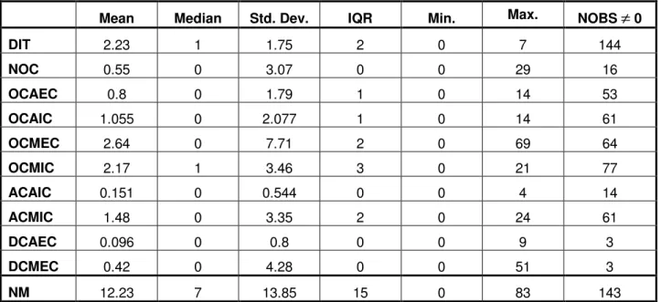
The descriptive statistics for the object-oriented metrics and the size measure for the Java data set are shown in Table 5. The table shows the mean, standard deviation, median, inter-quartile range (IQR), the minimum and maximum, and the number of observations that are not equal to zero. The set of metrics analyzed consists of two inheritance metrics, Depth of Inheritance Tree (DIT) and Number of Children (NOC) and eight coupling metrics, of which four are Import Coupling metrics (OCAIC, OCMIC, ACAIC, ACMIC) and four are Export Coupling metrics (OCAEC, OCMEC, DCAEC, DCMEC). A more detailed description of these metrics is given in the appendix.

Variables DCAEC and DCMEC have less than five observations that are non–zero. Therefore, we exclude them from further detailed analysis. The size metric we used was the number of methods in a class (NM).

Mean Median Std. Dev. IQR Min. Max. NOBS

≠

0

DIT 2.23 1 1.75 2 0 7 144 NOC 0.55 0 3.07 0 0 29 16 OCAEC 0.8 0 1.79 1 0 14 53 OCAIC 1.055 0 2.077 1 0 14 61 OCMEC 2.64 0 7.71 2 0 69 64 OCMIC 2.17 1 3.46 3 0 21 77 ACAIC 0.151 0 0.544 0 0 4 14 ACMIC 1.48 0 3.35 2 0 24 61 DCAEC 0.096 0 0.8 0 0 9 3 DCMEC 0.42 0 4.28 0 0 51 3 NM 12.23 7 13.85 15 0 83 143

Table 5: Descriptive statistics for all of the object-oriented metrics on the java data set.

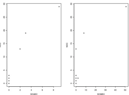
4.2 Testing the NOC Hypotheses

We expect that there will be no relationship between NOC and fault-proneness. Furthermore, we noted that there is a confounding effect between NOC and descendant-based export coupling. We saw from the descriptive statistics above that only three classes have descendant type export coupling. Therefore we cannot construct a model controlling for the effect of Descendant-based coupling. However, Figure 5 shows that the few classes with the largest NOC values will have greater descendant-based coupling.

DCAEC N O C 0 2 4 6 8 0 5 1 0 1 5 2 0 2 5 3 0 DCMEC N O C 0 10 20 30 40 50 0 5 1 0 1 5 2 0 2 5 3 0

Figure 5: Relationship between descendant based export coupling and number of children.

The results of a formal test of hypothesis are presented in Table 6. These indicate that there is a statistically significant effect of NOC on fault-proneness. However, this includes the confounding effect of descendant-based export coupling. Since we cannot explicitly control for this type of export coupling because the metrics have a very low variation, we removed one observation with the largest value of descendant-based export coupling from the data set, this renders the NOC to fault-proneness association non-significant at an alpha level of 0.05. Therefore the positive association between NOC and fault-proneness is dependent on the fact that the largest NOC values are also the largest descendant-based export coupling values. This result is as expected.

G R2 33.14 (2 d.f.); p < 0.0001 0.21 Intercept NM NOC Coefficient -2.41 0.08 0.309 p-value <0.0001 <0.0001 0.049

∆Ψ

3.03 2.59

Table 6: Logistic regression results for testing the NOC hypotheses.

4.3 Testing the DIT Hypotheses

To test the DIT hypotheses we only need to construct two models, a linear and a quadratic one. Since these are nested models, they can be compared using a likelihood ratio statistic (see Eqn. 7 vs. Eqn. 8 below):

( )

NM

DIT

( )

2 3 2 1 0

NM

DIT

DIT

logit

π

=

β

+

β

+

β

+

β

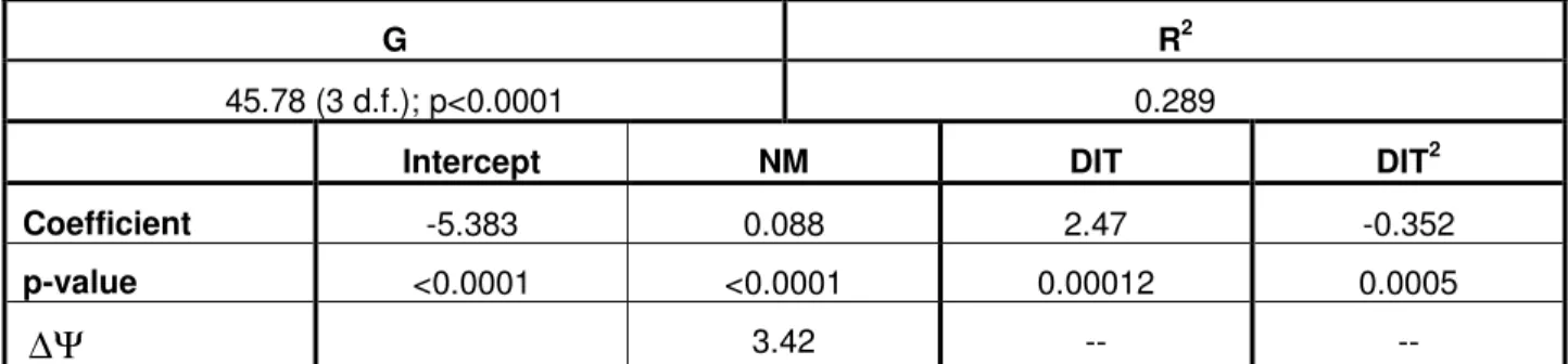
_{Eqn. 8}

The results for the DIT hypotheses are shown in Table 7. The parameter for the quadratic term is statistically significant.9 Since this is based on a likelihood ratio test, it indicates that the quadratic model is preferred over the linear model. Therefore, the evidence supports the quadratic hypothesis. We do not show the change in odds ratio for the DIT metric because the change

depends on the specific value of DIT, and hence no single universal

∆Ψ

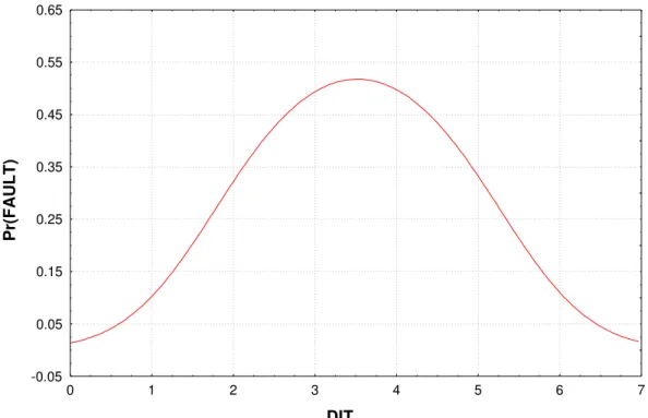
value for DIT makes

sense. Figure 6 shows the relationship between DIT and fault-proneness. This indicates that the impact of DIT depends on the value of DIT (i.e., for values of DIT below the peak the change in odds ratio will be greater than one, and for values of DIT above the peak the change in odds ratio will be below one). This plot also shows that the results strongly support the familiarity mechanism postulated earlier.

G R2

45.78 (3 d.f.); p<0.0001 0.289

Intercept NM DIT DIT2

Coefficient -5.383 0.088 2.47 -0.352

p-value <0.0001 <0.0001 0.00012 0.0005

∆Ψ

3.42 --

--Table 7: Logistic regression results for testing the DIT hypotheses.

9

DIT P r(F A U L T ) -0.05 0.05 0.15 0.25 0.35 0.45 0.55 0.65 0 1 2 3 4 5 6 7

Figure 6: Relationship between DIT and the probability of a post-release fault at the mean value

of NM.

4.4 Testing the Export Coupling Hypotheses

It was noted in Section 3.3 that inheritance metrics may be confounded with coupling metrics. Therefore, to test the export coupling hypotheses, we need to control for the potential confounding effect of inheritance depth. Recall that, if in this particular system there is no confounding effect, the inclusion of the inheritance depth variable in the model will not affect the estimates for the export coupling metrics. However, if there is a confounding effect then the parameter estimates will be more accurate.

We formulate the following two models for the export coupling metrics:

( )

NM

DIT

DIT

OCAEC

logit

π

=

β

₀

+

β

₁

+

β

₂

+

β

₃ 2

+

β

_{4 Eqn. 9}

( )

NM

DIT

DIT

OCMEC

logit

2 ₄ 3 2 1 0

β

β

β

β

β

π

=

+

+

+

+

Eqn. 10

G R2

50.87 (4 d.f.); p<0.0001 0.323

Intercept NM DIT DIT2 OCAEC

Coefficient -5.78 0.091 2.62 -0.37 0.32

p-value <0.0001 <0.0001 0.00013 0.0005 0.037

∆Ψ

3.5 -- -- 1.59

Table 8: Logistic regression results for testing the OCAEC hypotheses.

G R2

53.8 (4 d.f.); p<0.0001 0.347

Intercept NM DIT DIT2 OCMEC

Coefficient -6.3 0.085 3.24 -0.49 0.077

p-value <0.0001 <0.0001 0.000016 0.00006 0.039

∆Ψ

3.28 -- -- 1.81

Table 9: Logistic regression results for testing the OCMEC hypotheses.

The results are shown in Table 8 and Table 9. They indicate that the export coupling metrics have a statistically significant association with post-release fault proneness. According to our

hypotheses, these indicate that the familiarity hypothesis cannot be supported,10 and that the

interference and fan effects hypotheses receive empirical support.

4.5 Testing the Import Coupling Hypotheses

In a manner similar to the export coupling metrics, we formulate two models that control for the effect of inheritance depth:

( )

NM

DIT

DIT

OCAIC

logit

π

=

β

₀

+

β

₁

+

β

₂

+

β

₃ 2

+

β

_{4 Eqn. 11}

( )

NM

DIT

DIT

OCMIC

logit

4 2 3 2 1 0

β

β

β

β

β

π

=

+

+

+

+

Eqn. 12 10

It is plausible that a familiarity effect exists, but its magnitude is small, and is cancelled by the competing positive effect. However, it is only possible to conjecture that this may be the case from this study.

G R2

57.74 (4 d.f.); p<0.0001 0.37

Intercept NM DIT DIT2 OCAIC

Coefficient -6.7 0.057 4.14 -0.72 0.47

p-value <0.0001 0.016 <0.0001 <0.0001 0.0042

∆Ψ

2.19 -- -- 2.68

Table 10: Logistic regression results for testing the OCAIC hypotheses.

G R2

63.62 0.41

Intercept NM DIT DIT2 OCMIC

Coefficient -6.03 0.053 2.38 -0.31 0.379

p-value <0.0001 0.048 0.0004 0.002 <0.0001

∆Ψ

2.11 -- -- 3.73

Table 11: Logistic regression results for testing the OCMIC hypotheses.

The results of testing these hypotheses are shown in Table 10 and Table 11. These indicate a strong positive and statistically significant relationship between these import coupling metrics and post-release fault-proneness.

Now we consider the ancestor-based import coupling. The ACAIC metric had only 14 non-zero values, and almost all of these were one. Thus this variable had restricted variation. The results for testing the ACAIC metric hypotheses are shown in Table 12. This indicates that there is no relationship between ACAIC and post-release fault-proneness.

G R2

46.94 (4 d.f.); p<0.0001 0.298

Intercept NM DIT DIT2 ACAIC

Coefficient -5.33 0.085 2.48 -0.36 0.45

p-value <0.0001 <0.0001 0.0002 0.0007 0.37

∆Ψ

3.3 -- -- 1.22

Table 12: Logistic regression results for testing the ACAIC hypotheses.

Figure 7 shows the relationship between ACMIC and DIT. It is clear that ACMIC is largest in the middle of the inheritance hierarchy. Given that we found the greatest fault-proneness in the middle of the inheritance hierarchy, this indicates a strong confounding effect of DIT on ACMIC. The same pattern was observed for ACAIC, although not as pronounced. This confounding explains why ACAIC was not significant, after controlling for the effect of depth of inheritance tree.

DIT A C MI C 2 4 6 8 0 .0 0 .5 1 .0 1 .5 2 .0

Figure 7: Relationtship between median ACMIC and DIT.

Similar conclusions can be drawn about ACMIC as seen in Table 13. The ACMIC metric is not associated with post-release fault-proneness after controlling for inheritance depth. It should also be noted that, when we do not control for inheritance depth we get highly significant ACAIC and ACMIC effects. Therefore, it is important to be cognizant of the confounding effect of DIT when building and interpreting validation models.

A post-hoc power analysis determined that the likelihood ratio test statistical power for ACAIC was 17% and for ACMIC was 9%. These are quite low values, indicating that the test was not sufficiently powerful at these sample and effect sizes to identify a significant effect if one existed.

G R2

49.04 94 d.f.); p<0.0001 0.311

Intercept NM DIT DIT2 ACMIC

Coefficient -5.433 0.088 2.45 -0.347 0.075

p-value <0.0001 <0.0001 0.00058 0.0018 0.393

∆Ψ

3.39 -- -- 1.23

Table 13: Logistic regression results for testing the ACMIC hypotheses.

4.6 Building the Predictive Model

As noted earlier, we use a manual approach for selecting the metrics to include in the predictive model. Table 14 shows the correlations among the significant coupling metrics. As can be seen the export coupling metrics are strongly correlated with each other and so are the two import coupling metrics. We therefore select one of each type that had the largest change in odds ratio in the validation models above. This leaves us with OCMIC and OCMEC.

OCAEC OCMEC OCMIC OCAIC

OCAEC 1.00

OCMEC 0.54 1.00

OCMIC 0.21 0.19 1.00

OCAIC 0.31 0.30 0.51 1.00

Table 14: Correlations among the significant coupling metrics.

The final prediction model is shown in Table 15. The area under the ROC curve is 0.85 using a leave-one-out cross-validation. This can be considered a very good value indicating a high prediction accuracy.

G (p-value)

R2

65.7 (5 d.f.); p < 0.0001 0.42

NM DIT DIT2 OCMIC OCMEC

Coefficient 0.039 2.39 -0.318 0.3874 0.0826

p-value 0.185 0.00042 0.0023 <0.0001 0.016

∆Ψ

1.73 -- -- 3.829 1.89

Table 15: Logistic regression results for the best model.

4.7 Summary of Hypothesis Tests

In general, our results support the cognitive theory. We also witnessed a confounding effect of depth of inheritance tree on some of the coupling metrics. Therefore, it is prudent to control for inheritance depth when validating coupling metrics. Consistent evidence was found for interference and fan effects.

The substantive results can be summarized as follows:

NOC Hypotheses: We expected that NOC would not be associated with fault-proneness

after controlling for descendant-based export coupling. This was the results obtained, and is consistent with previous work.

DIT Hypotheses: Classes at the root of the hierarchy or that are deepest in the hierarchy

are most familiar because they are consulted often. Therefore, due to the familiarity, they will have a low fault-proneness compared to class in the middle of the hierarchy.

Export Coupling Hypotheses: Classes with high export coupling have many

assumptions made about their behavior. This can be considered a form of fan effect. Furthermore, more interference will occur as the engineers trace back frequently from classes with high export coupling to understand how they are used. This result is supportive of the cognitive hypothesis.

Import Coupling Hypotheses: Classes with high import coupling to other classes are

more fault-prone due to interference and fan effects. Ancestor-based import coupling is not related with fault-pronensss. However, this result may be due to the low statistical power of the current study.

It is worthwhile to point out that most of our results are congruent with previous research. One exception is the quadratic relationship with DIT. There are two explanations for this. First,

previous studies did not look for a quadratic relationship.11 Second, in previous studies DIT did not vary very much due to the lack of use of inheritance. This would explain why a quadratic relationship may not be found, even if the authors attempted to look for it.

Another exception is that some previous studies did not find a relationship between import coupling between classes and fault-proneness (El-Emam et al., 1999). This may be due to these studies not controlling for the effect of inheritance depth. Similarly, previous studies found an effect for ancestor-based import coupling and we did not. We noted a confounding effect of DIT and the ancestor-based import coupling metrics, and this was not accounted for in previous studies. This explains the difference in findings.

4.8 Potential Cost Savings from Using the Prediction Model

We used a leave-one-out technique to estimate the potential cost savings from using the prediction model. As noted earlier, this would give us a realistic estimate of the values in the confusion matrix should the prediction model be applied on a future system. We use Eqn. 8 to compute the cost savings.

Most Faulty x% C o st S a v in g s 0.1 0.2 0.3 0.4 0.5 0 .3 0 0 .3 5 0 .4 0

Figure 8: Cost savings from applying the prediction model by using PBR inspections on the top

x% classes in terms of predicted fault-proneness for a cost ratio of 4. This is a smoothed plot. A graph showing the cost savings is given in Figure 8. The x-axis shows the percentage of classes the project manager decides to inspect based on the predicted fault-proneness of the prediction model. For example, if the project manager had selected the top 39% of classes for

inspections12 using the prediction model, approximately 42% of total post-release costs would be

saved. For this organization, this would translate to a significant amount of cost savings given that post-release costs can be quite large. A slightly higher cost saving would have been obtained had the project manager known that only 23% of the classes were faulty for this particular product. Furthermore, note that in our formulation and selection of values we have deliberately tended to be conservative so as not to exaggerate the benefits of the prediction model. Therefore, it is plausible that benefits would be higher.

In principle, the savings model that we have presented can be used to evaluate the benefits when applying other fault detection techniques or combinations of them. Our application used inspections with PBR reading since this particular technique was of interest to the organization.

11

At least this was not mentioned in published studies.

12

This is the value that the project manager would reasonably use based on a previous similar project by the same team (El-Emam et al., 2001b)