Environmental Satisfaction in Open-Plan Environments: 6. Satisfaction Algorithms for Software

Publisher’s version / Version de l'éditeur:

Questions? Contact the NRC Publications Archive team at

PublicationsArchive-ArchivesPublications@nrc-cnrc.gc.ca. If you wish to email the authors directly, please see the first page of the publication for their contact information.

https://publications-cnrc.canada.ca/fra/droits

L’accès à ce site Web et l’utilisation de son contenu sont assujettis aux conditions présentées dans le site LISEZ CES CONDITIONS ATTENTIVEMENT AVANT D’UTILISER CE SITE WEB.

Research Report (National Research Council of Canada. Institute for Research in

Construction), 2004-04

READ THESE TERMS AND CONDITIONS CAREFULLY BEFORE USING THIS WEBSITE.

https://nrc-publications.canada.ca/eng/copyright

NRC Publications Archive Record / Notice des Archives des publications du CNRC :

https://nrc-publications.canada.ca/eng/view/object/?id=086d98b5-42b8-46a7-b998-7f66785bb570 https://publications-cnrc.canada.ca/fra/voir/objet/?id=086d98b5-42b8-46a7-b998-7f66785bb570

Archives des publications du CNRC

For the publisher’s version, please access the DOI link below./ Pour consulter la version de l’éditeur, utilisez le lien DOI ci-dessous.

https://doi.org/10.4224/20378548

Access and use of this website and the material on it are subject to the Terms and Conditions set forth at

Environmental Satisfaction in Open-Plan Environments: 6. Satisfaction

Algorithms for Software

Newsham, G. R.; Veitch, J. A.; Charles, K. E.; Marquardt, C. J. G.; Geerts,

J.; Sander, D. M.

Environmental Satisfaction in Open-Plan Environments:

6. Satisfaction Algorithms for Software

Newsham, G.R.; Veitch, J.A.; Charles, K.E.;

Marquardt, C.J.G.; Geerts, J.; Sander, D.

IRC-RR-155

April 2004

Environmental Satisfaction in Open-Plan Environments: 6. Satisfaction Algorithms for Software

Guy R. Newsham, Jennifer A. Veitch, Kate E. Charles, Clinton J.G. Marquardt, Jan Geerts, Dan Sander

Executive Summary

One of the outcomes of the COPE project is software to aid decision-makers in the design and operation of open plan offices. The software concept is that decision-makers enter key aspects of the office design; e.g., cubicle size, partition height, ceiling tile properties, surface

reflectances. They also provide costing information related to these choices. The software accesses the results of the other COPE study tasks to indicate expected indoor environment

conditions associated with these choices, such as illuminance, speech privacy and glare. These can be compared with particular criteria that might apply. The software will also indicate

potential occupant satisfaction issues (‘positives’ or ‘negatives’) associated with the design, and provide text advice on these issues. This report details the derivation of the algorithms (or

‘rules’ or ‘heuristics’) that determine under what conditions occupant satisfaction issues are identified.

To determine which physical parameters might be associated with satisfaction effects we looked to three sources: regressions from our field study data, other published studies, and

existing recommended practice documents. Then we calculated what percentage of occupants in our field study sample were Highly Satisfied or Highly Dissatisfied with Lighting, Privacy, or Ventilation (as appropriate) at each

level of that physical variable. From this we determined at what values of the physical variable there was a transition from greater membership in the Highly Satisfied group to greater membership in the Highly Dissatisfied group. An example for cubic illuminance (the mean of six illuminances measured on each

face of a cube at the location of a seated occupant’s head) with respect to Satisfaction

with Lighting is shown in Figure ES1. In the example, there is a greater probability of being in the Highly Satisfied group, as opposed to the Highly Dissatisfied group, for cubic illuminances

between 120 – 240 lx. This translates into desktop illuminances between 275 – 490 lx,

which is similar to the suggested values for offices in many recommended practice

documents.

We used this process for several other physical parameters, which led to the satisfaction effects

shown in Table ES1. These effects will be implemented in the COPE software tool. All of

these effects are supported by evidence from other sources. Decision-makers might want to consider remedial action for designs that accumulate a large number of negative satisfaction

effects.

Figure ES1. Percentage of occupants (with no appreciable daylight) at each level of cubic illuminance that was highly satisfied or highly dissatisfied with Lighting. Quadratic fits to the data

points are also shown.

0 5 10 15 20 25 30 35 <8 0 80-120 120-160 160-200 200-240 240+ ecube % sam p le Satisfied Dissatisfied (lx)

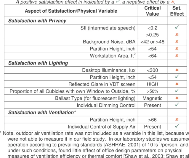
Table ES1. Satisfaction effects associated with various levels of important physical variables. A positive satisfaction effect in indicated by a _!, a negative effect by a _".

Aspect of Satisfaction/Physical Variable Critical Value

Sat. Effect Satisfaction with Privacy

SII (intermediate speech) <0.2

!

>0.25

"

Background Noise, dBA <42 or >48

"

"

_"

Desktop Illuminance, lux <300

_"

!

"

Proportion of all Cubicles with own Window to Outside, % >50%

!

Ballast Type (for fluorescent lighting) Magnetic

_"

!

Partition Height, inch >66

"

!

were not able to measure it in our field study. In our laboratory studies we assumed operation according to prevailing standards [ASHRAE, 2001] of 10 ls-1/person, and, under such conditions, found little effect of office design parameters on physical measures of ventilation efficiency or thermal comfort [Shaw et al., 2003; Shaw et al., 1993]. A review of the literature indicates that outdoor air rates of less than 10 ls-1/person are likely to increase the risk of occupant dissatisfaction with ventilation [Charles and Veitch, 2002].

We also used the same process for physical parameters not currently calculated by the software. This revealed possible interesting effects, also supported by other sources, of

illuminance uniformity on Satisfaction with Lighting, and carbon-dioxide concentration, temperature, and air velocity on Satisfaction with Ventilation.

Table of Contents

1.0 Introduction... 5

2.0 Method ... 6

3.0 Results ... 9

3.1 Satisfaction with Privacy... 10

3.2 Satisfaction with Lighting... 15

3.3 Satisfaction with Ventilation... 21

4.0 Discussion ... 25

5.0 References ... 27

1.0 Introduction

One of the outcomes of the COPE project is software to aid decision-makers in the design and operation of open plan offices. The software concept is that decision-makers enter key aspects of the office design; e.g., cubicle size, partition height, ceiling tile properties, surface

reflectances. They also provide costing information related to these choices. The software accesses the results of the other COPE study tasks to indicate expected indoor environment

conditions associated with these choices, such as illuminance, speech privacy and glare. These can be compared with particular criteria that might apply. The software will also indicate

potential occupant satisfaction issues (‘positives’ or ‘negatives’) associated with the design, and provide text advice on these issues. This report details the derivation of the algorithms (or

‘rules’ or ‘heuristics’) that determine under what conditions occupant satisfaction issues are identified.

There have been many attempts to associate physical conditions with occupant satisfaction for individual physical parameters (e.g., desktop illuminance, temperature), and many references to these are given in the following sections. We believe this is the first attempt to integrate so

many satisfaction issues into a coherent group to cover indoor environment issues more broadly. Whereas for some variables (e.g., temperature) relationships to occupant satisfaction

are well-established with high resolution, the same is not true for most other variables (e.g. desktop illuminance). After consultation with the COPE consortium, we chose a relatively simple categorization scheme for satisfaction effects that allowed us to consider all effects in

2.0 Method

The starting point for the development of the algorithms was analysis of data collected during a field study of nine buildings in six cities. Six of these buildings were in Canada, and three in

the US; three were federal buildings, two were provincial buildings, and four were private-sector (high tech) buildings. A total of 779 employees and their workstations were included in

the data set. During a workstation visit, research staff conducted detailed measurements of ventilation, temperature, noise, lighting, and descriptive characteristics of the workstation during a 10-minute period. At the same time, the occupant completed a 27-item questionnaire on a handheld computer concerning their satisfaction with the workplace. The methodology of these studies and descriptive data from the various study sites has been detailed elsewhere [Veitch et al, 2002a]. Using these data, we conducted a series of regression studies [Veitch et

al., 2003], which examined the relationships between physical descriptors of the indoor environment and occupant environmental satisfaction. Separate scales for satisfaction with

lighting, privacy, and ventilation were considered [see Table 1 for definitions]. Our interest in this report is to develop algorithms that can be used to provide satisfaction

predictions for a given cubicle design. Our goal is therefore to decide what levels of satisfaction should be ascribed to what levels of a physical variable. At a previous meeting with project sponsors we decided on the simple approach of assigning positive and negative

points for various aspects of the physical environment related to a particular aspect of satisfaction. This is very similar to the point award system for environmental features in the popular LEED programs [USGBC]. For example, with respect to satisfaction with lighting, we might ascribe a positive point for having a window, a negative point for glare, a negative point

for an illuminance outside of a certain illuminance range, and so on. Our challenge is to determine how such points might be awarded for all aspects of satisfaction, and for all relevant

physical variables. Our general philosophy was to use the field study data and regression analyses as our primary source of guidance (because it was collected from real employees in

real buildings), and to supplement this with the results of other studies by ourselves and others, and more qualitative expert opinion.

Simply using the relationships from the regression analyses alone did not seem very suitable as it requires the assumption of a given level (or levels) of satisfaction to define critical levels of a physical variable: should we use the middle of the satisfaction scale to define the critical level, or something else? Also, the regression lines generally have low slopes, indicating that average satisfaction does not vary much with changes in physical parameters. This makes it difficult to argue that a particular level of physical parameter is especially important. These

considerations suggested a different approach.

First, rather than looking at average satisfaction, we decided to focus more at the extremes, looking at the differences in physical conditions experienced by the highly satisfied and the highly dissatisfied occupants. After considering several schemes to identify these two groups,

we settled on defining the “Highly Satisfied” for a particular aspect of satisfaction as those participants with satisfaction votes in the top 20% of all votes, and the “Highly Dissatisfied” as

those in the bottom 20%. These groups were defined separately for each satisfaction scale. The choice of the bottom 20% defining dissatisfaction echoes the 20% dissatisfaction target

accepted as the minimum level of acceptable thermal comfort that is commonly in use in practice [ASHRAE, 1992; ISO, 1994].

Next, we found the points on the satisfaction scale that define these two groups for the whole sample. For example, for Satisfaction with Privacy, the bottom 20% of ratings are at a value of

higher. Next, for each level1 of a particular physical parameter we calculated the percentage of all ratings made at that level of the parameter that were above 4.9, and the percentage

below 2.9. We then plotted those points on a graph and drew trend lines through them. Finally, the points at which those trend lines cross indicate possible critical levels of the physical parameter, levels at which there is a transition to there being more people in the

Highly Satisfied group than the Highly Dissatisfied group (or vice versa).

Before looking at the results of this process with our data, consider a simple example from another context to illustrate the concept. Consider the notional relationship between satisfaction with a beach vacation and the number of sunshine hours for that beach in a year (see Figure 1). Look first at Figure 1(a). We would expect that at very low levels of sunshine the number of people with particularly low ratings of satisfaction (“Highly Dissatisfied”) would be high, but would decline with increasing number of sunshine hours. Conversely, we would expect that at very low levels of sunshine the number of people with particularly high ratings of

satisfaction (“Highly Satisfied”) would be low, and would increase with increasing number of sunshine hours. Figure 1(a) illustrates linear relationships for each of these trends. The point

at which these trend lines cross defines a critical level of sunshine hours (SHcrit). For any number of sunshine hours above SHcrit the number of Highly Satisfied people outweighs the

number of Highly Dissatisfied people. To take the analogy one step further, to planning advice, a developer could use this information in making investment decisions about the siting

of resorts with reference to climate data.

Relationships between satisfaction and physical parameters are not always simple linear ones, of course. One might imagine that too much sunshine could also be a bad thing, in this case

the appropriate relationship might look more like Figure 1(b). In this example we have two crossover points, and two values of SHcrit that define a preferred zone.

As we will see in the Results section, the trend lines from our field study data are rarely as clearly defined as in the examples of Figure 1. People are relatively insensitive to certain

physical parameters, and there is variability in the data due to measurement error and confounds between parameters that are inevitable in real buildings. Note that this approach does not include statistical tests of differences between groups. Therefore, wherever possible, we will present evidence from other studies to support the derivations of critical values from the

field study data.

1

Because the physical variables were generally continuous variables, we binned the physical data at simple intervals, with a reasonable sample size in each bin.

Sunshine hours Freq., % 0 100 SHcrit Highly Satisfied Highly Dissatisfied Sunshine hours Freq., % 0 100 SHcrit Highly Satisfied Highly Dissatisfied SHcrit

Figure 1. The notional relationship between satisfaction with a beach vacation, and number of sunshine hours, illustrating how critical values of a physical parameter can be derived,

from consideration of the effect on highly satisfied and dissatisfied groups. (a) illustrates a linear relationship; (b) illustrates a quadratic relationship

3.0 Results

The results are divided into sections by aspects of satisfaction: privacy, followed by lighting, followed by ventilation. Table 1 describes the dependent and independent variables referred

to in this study, and Table 2 gives descriptive statistics for each of the variables. Table 1. Description of the dependent and independent variables addressed in these analyses.

Variable Name Unit

(or range)

Description Independent Variables

LNOISEA dB(A) A-weighted background noise level at approximately the position of a seated occupant’s head, measured during the day.

SII 0 – 1 Speech Intelligibility Index, calculated from an assumed intermediate speech level [Bradley, 2003], the sound propagation between

workstations measured at night, and LNOISEA

E_CUBE lux The mean illuminance on the six sides of a cube at approximately the position of a seated occupant’s head, measured during the day. E_DESK lux Mean illuminance at four points on desktop, measured during the day. E_DESKUNI 0 – 1 (Maximum of four desktop illuminance points – Minimum of same four

points) / Maximum (therefore, higher values are less uniform) RTD_H oC Air temperature measured during the day 1.1 m from the ground, at

the approximate location of a seated occupant’s head.

AIR_V_H ms-1 Air velocity measured during the day 1.1 m from the ground, at the approximate location of a seated occupant’s head.

FDCO2 ppm Carbon-dioxide concentration at approximately the position of a seated occupant’s head, measured during the day.

SQRTAREA ft Square root of the workstation area, rather than area itself because it is better distributed, and better facilitates comparison to non-field studies.

MINPH_NOOPEN inch The minimum (non-zero) partition height of all partitions making up the cubicle, but excluding any fully open sides.

WINDOW 0, 1 =1 if the cubicle contained an external window; =0 if it did not. DAYLIGHT 0, 1, 2 =2 if the cubicle contained an external window; =1 if it did not have a

window but was within 15ft of a window; =0 if the cubicle was more than 15ft from a window. (treated as a numerical variable in analyses) VDT_CAT Low,

Medium, High

Determined from a photograph of the computer screen (switched off) in each cubicle. Categorized in 3 levels by visual inspection: LOW (no substantial reflections); MEDIUM (small fraction of screen affected by reflections); and, HIGH (large fraction of screen affected by reflections)

Dependent Variables

SATPRIV 1 – 7 Satisfaction with Privacy, mean of occupant responses to ten questions on satisfaction with: workstation size, degree of enclosure, ability to alter conditions, visual privacy, privacy for conversations in your office, noise from other people’s conversations, background noise, frequency of distractions, distance from co-workers, and aesthetic appearance. Each question used a seven-point scale, ranging from “very unsatisfactory” (1) to “very satisfactory” (7). [Charles et al., 2003]

SATLIGHT 1 – 7 Satisfaction with Lighting, mean of five questions on satisfaction with: the amount of light for computer work, glare in the computer screen, access to a view, quality of lighting, and overall lighting on the desktop.

SATVENT 1 – 7 Satisfaction with Ventilation, the mean of three questions on satisfaction with: air quality, temperature, and air movement.

Table 2. Descriptive statistics for the whole sample for variables in these analyses. s.d. = standard deviation.

Variable Name Unit

(or range)

N Min. Max. Medn. Mean s.d.

Independent Variables LNOISEA dB(A) 729 36.2 56.8 46.6 46.3 3.6 SII 0 – 1 729 0.08 0.91 0.51 0.51 0.15 E_CUBE lux 770 9 911 202 243 151 E_DESK lux 770 4 1654 400 447 239 E_DESKUNI 0 – 1 779 0.01 1.00 0.41 0.43 0.20 RTD_H oC 770 20.5 26.1 23.3 23.2 0.9 AIR_V_H ms-1 766 0.01 0.25 0.08 0.09 0.04 FDCO2 ppm 767 470 935 638 643 87 SQRTAREA ft 778 3.5 14.5 8.7 8.9 2.0 MINPH_NOOPEN inch. 776 36 81 64 61 9.5 Categories (N) 0 1 2 WINDOW 461 318 DAYLIGHT 330 131 318

Low Med. High

VDT_CAT 336 163 274

Unit (or range)

N Min. Max. Medn. Mean s.d.

Dependent Variables

SATPRIV 1 – 7 775 1.0 6.7 3.9 3.8 1.1

SATLIGHT 1 – 7 776 1.4 7.0 5.0 4.8 1.2

SATVENT 1 – 7 775 1.0 7.0 4.3 4.2 1.4

3.1 Satisfaction with Privacy

To illustrate the method, we will describe the derivation of critical SII values on Satisfaction with Privacy (SatPriv) in detail. In fact, there was a lack of a relationship between SII and SatPriv in the field study regression analysis. In most cases, this would discourage us from continuing the analysis further. However, results from other sources supporting a relationship,

including our own laboratory study [Veitch et al., 2002b] are so consistent that in this case we pursued the derivation of critical values from the field study data. SII’s were grouped into bins

of 0.1 in size. The top 20% of SatPriv ratings were >4.9, and the bottom 20% were <2.9, defining the Highly Satisfied and Highly Dissatisfied groups respectively. For each SII bin, we calculated the percentage of votes that were >4.9, and <2.9, as shown in Table 3. These are then plotted, with linear trends, as shown in Figure 2. Linear trends are chosen because the expected tendency is for the fraction of Highly Satisfied people to increase as SII declines, and

Table 3. The number of Satisfaction with Privacy scores within certain ranges at each level of SII. Also shown are the scores in the Highly Satisfied (>4.9) and Highly Dissatisfied (<2.9)

ranges as a percentage of all scores at each level of SII.

SatPriv Scores

Frequencies Percentages

SII (int.) <2.9 2.9 to 4.9 >4.9 Total <2.9 >4.9

<0.2 12 69 17 98 12.2 17.3 0.2-0.3 24 89 30 143 16.8 21.0 0.3-0.4 47 93 41 181 26.0 22.7 0.4-0.5 29 103 29 161 18.0 18.0 >0.5 29 102 20 151 19.2 13.2 Total 141 456 137 734 0 5 10 15 20 25 30 <. 2 .2 -. 3 .3 -. 4 .4 -. 5 >. 5 SII (intermediate) % sam p le

Figure 2. Percentage of the sample at each level of SII that was highly satisfied or highly dissatisfied with Privacy. Linear fits to the data points are also shown.

Satisfied Dissatisfied

The lines defining the linear trends cross at approximately 0.3 – 0.35 on the SII scale. For SII lower than this value there is a greater tendency for individuals to be in the Highly Satisfied

group rather than the Highly Dissatisfied group. Nevertheless, we know from other work [Veitch et al., 2002b] that an SII of less than 0.2 is also suggested for speech privacy to be considered acceptable. In recent work, Bradley and Gover [2003] showed that 50% of people

can understand ~90% of the words from an adjacent office at a calculated SII of 0.25. Therefore, in the context of an open-plan office, we suggest that an SII<0.2 indicates a positive condition for Satisfaction with Privacy; 0.2≤SII≤0.25 is neutral; and, SII>0.25 is a

negative condition. Using the symbols

"

!

for a positive

SII

< 0.2

!

> 0.25

"

We then followed the same process for other variables related to Satisfaction with Privacy, beginning with background noise levels (LNOISEA). Again, regressions from field study data

showed no significant relationship between background noise and SatPriv scores. Nevertheless, there is considerable evidence from other studies that a relationship does exist

[Veitch et al., 2002b; Navai and Veitch, 2003]. The relationship suggested by these other studies is quadratic, with too little background noise not providing enough sound masking, and

too much background noise being annoying in itself. We therefore pursued a quadratic relationship for the Highly Satisfied and Highly Dissatisfied groups, shown in Figure 3. The curve fits are quite good, and generally support suggestions from other studies [Veitch et al.,

2002b; Navai and Veitch, 2003]. Considering all sources of information, we propose the desired range of background noise level is 42–48 dBA. As suggested above, we consider

background noise level on either side of this range to be associated with a negative satisfaction condition. Noise levels within the range provide some sound masking, and might lead to positive outcomes for SII, but can only be considered as a neutral satisfaction condition

for background noise itself. Therefore, the algorithm relating Satisfaction with Privacy to background noise can be summarized as:

Background

Noise (dBA)

< 42

_"

> 48

"

One would expect partition height (MINPH_NOOPEN) to be associated with privacy, both through acoustic and visual privacy. Again, regressions from field study data showed no significant relationship between partition height and SatPriv scores. Nevertheless, there is evidence from other studies that a relationship does exist between partition height/enclosure and measures of satisfaction [Marquardt et al., 2002; Brill, 1984; Oldham, 1988; Oldham and

Fried, 1987]. There is no theoretical reason to consider anything other than a linear relationship, and the result for the Highly Satisfied and Highly Dissatisfied groups is shown in Figure 4. The curve fits are imperfect, but are in the directions expected. The crossover point

condition. Therefore, the algorithm relating Satisfaction with Privacy to partition height can be summarized as: Min. Partition Ht. (in.) < 54

"

Finally, regressions from our field study data showed a significant relationship between workstation size (SQRTAREA) and SatPriv scores. This is consistent with the limited literature

on the topic of occupant density and environmental satisfaction [Duval et al., 2002]. We explored the relationship for the Highly Satisfied and Highly Dissatisfied groups in our field study data, and the result is shown in Figure 5. There is no theoretical reason to pursue a quadratic relationship, however, quadratic curves do provide a much better fit to the data points. Even so, because of the lack of theoretical support, we treat the crossover point at larger workstation sizes as an artefact of the curve fitting. The lower crossover point suggests

a critical workstation size of 8 ft x 8 ft (64 ft2). We consider a workstation smaller than this value to be associated with a negative Satisfaction with Privacy condition, and workstations

bigger than this as a neutral condition. Therefore, the algorithm relating Satisfaction with Privacy to workstation area can be summarized as:

WS Size (ft) < 8 x 8

_"

0 5 10 15 20 25 <4 0 40-44 44-48 48-52 >5 2 LnA (dB) % s a m p le Satisfied Dissatisfied

Figure 3. Percentage of the sample at each level of background noise that was highly satisfied or highly dissatisfied with Privacy. Quadratic fits to the data points are also shown.

0 5 10 15 20 25 30 <7 _7-8 _8-9 9-1 0 10-1 1 11-1 2 >12 SQRTAREA (ft) % s a m p le Satisfied Dissatisfied

Figure 5. Percentage of the sample at each level of workstation size that was highly satisfied or highly dissatisfied with Privacy.

Quadratic fits to the data points are also

0 5 10 15 20 25 30 35 40 <4 8 48-54 54-60 60-66 66-72 _>72 min PH % sam p le Satisfied Dissatisfied

Figure 4. Percentage of the sample at each level of minimum partition ht. that was highly satisfied or highly dissatisfied with Privacy. Linear fits to the data points are also shown.

3.2 Satisfaction with Lighting

Our field study data, and other research in the literature [Boubekri and Haghighat, 1993; Christoffersen et al., 2000; Finnegan and Solomon, 1981; Leather et al., 1998], show that one

of the biggest single influences on environmental satisfaction is proximity to a window. Regressions on our field study data [Veitch et al., 2003] reveal several significant effects relating the physical environment to Satisfaction with Lighting (SatLight) scores, but by far the biggest effect is proximity to a window. For algorithm development, it is clear that windows will

be associated positively with satisfaction. Our goal was to find other physical conditions, independent of window effects, that might influence Satisfaction with Lighting. Therefore, in

most cases, we conducted the procedure for examining differences in physical conditions experienced by the Highly Satisfied and Dissatisfied groups for workstations with no appreciable daylight (DAYLIGHT=0, i.e., workstations more than 15ft from a window), a sample of 327 workstations. For this sample the top 20% of SatLight scores were >5.5, and the bottom

20% were <3.2, defining the Highly Satisfied and Highly Dissatisfied groups respectively2. One would expect light level (illuminance) to be associated with Satisfaction with Lighting, and

regressions from our field study data suggest illuminance as a predictor of SatLight scores. Newsham and Veitch [2001] demonstrated that preferred desktop illuminances lie in the range

200-500 lx in a non-daylit office, and that exposing individuals to light levels substantially different from their preference led to satisfaction penalties. Recent research on occupant preference for illuminance in non-daylit offices suggests that both too little and too much light

can be unsatisfactory. In laboratory studies [Veitch & Newsham, 2000; Boyce at al., 2000; Berrutto et al., 1997], few participants consistently chose illuminances at either extreme available to them. In a field study of interior offices [Maniccia et al., 1999], two-thirds of occupants did operate lights at full-on, but a large minority (one-third) chose a dimmed setting.

This suggests a quadratic relationship between illuminance and satisfaction might be most appropriate.

We therefore pursued a quadratic relationship for the Highly Satisfied and Highly Dissatisfied groups, shown in Figure 6; the curve fits are good. The measure of illuminance used in this analysis was E_CUBE. We also measured the more familiar desktop illuminance (E_DESK) in

the field. E_CUBE and E_DESK are highly correlated (r=0.74) such that E_CUBE can be converted to E_DESK with confidence. The crossover points in Figure 6 are at E_CUBE = 120

lx and 240 lx, which translates to E_DESK = 275 lx and 490 lx. This is remarkably close to the IESNA recommendation for desktop illuminance in office spaces with VDTs [IESNA, 2000] of

300 – 500 lx. Therefore, we consider E_DESK<300 lx to represent a negative condition for Satisfaction with Lighting. We have chosen not to penalize desktop illuminances greater than

500 lx because these higher levels might be appropriate for some types of non-computer-based work and/or for localized task lighting. Therefore, the algorithm relating Satisfaction with

Lighting to desktop illuminance can be summarized as:

E_DESK (lx)

<300

"

Regressions from our field study data also suggest partition height (MINPH_NOOPEN) as a predictor of SatLight scores, with lower partition heights associated with higher SatLight scores. This might be partly due to an association between lower partitions and increased

2

window access and higher illuminance [Newsham and Sander, 2002; Reinhart 2002], both of which are also associated with higher satisfaction. Nevertheless, we will pursue partition height as a separate predictor. There is no theoretical reason to consider anything other than a

linear relationship, and the result for the Highly Satisfied and Highly Dissatisfied groups is shown in Figure 7. The critical value for minimum partition height is at ~ 54 inch, at heights lower than this the chances of being in the Highly Satisfied group are greater than the chances

of being in the Highly Dissatisfied group, and we associate positive satisfaction with this condition. Higher partition heights are not penalized directly, though they may incur a penalty

via their effect on illuminance. Therefore, the algorithm relating Satisfaction with Lighting to partition height can be summarized as:

Min. partition ht.

(in.)

<54

_!

Note that this algorithm is the exact opposite of the algorithm relating partition height to Satisfaction with Privacy. This illustrates the conflicting nature of some aspects of office

design.

The regressions on our field study data indicate no statistically significant relationship between workstation size and Satisfaction with Lighting. Although other work demonstrates an effect of

workstation size on illuminance [Newsham and Sander, 2002], there are no other sources suggesting an effect on satisfaction, and therefore we did not develop this relationship further.

Several studies have demonstrated an effect of VDT screen glare (VDT_CAT) on occupants’ satisfaction with their lit environment, and vision-related health symptoms [Veitch and

Newsham, 1998; Veitch and Newsham 2000; Lorusso et al., 2001]. The regressions performed on our field study data also indicate a significant relationship. This scale for VDT_CAT is not numerical, and therefore in Figure 8, rather than plotting a linear or quadratic

fit to the data, we present simply the percentage of Highly Satisfied and Highly Dissatisfied people at each glare condition. The percentage of Highly Dissatisfied people increases with increasing glare, as expected. The percentage of Highly Satisfied people unexpectedly peaks at the MEDIUM glare condition before dropping considerably at the HIGH glare condition. The

two groups only differ substantially at the HIGH glare condition. Therefore we assign a negative satisfaction condition to cases where the VDT has substantial reflected glare. The other glare conditions do not offer anything positive in terms of satisfaction, only an absence of

something bad, and are considered neutral with respect to satisfaction. Therefore, the algorithm relating Satisfaction with Lighting to VDT glare can be summarized as:

VDT Glare LOW MEDIUM

HIGH

"

As stated earlier, we expect the effect of windows/daylight on Satisfaction with Lighting to be large, and the regressions performed on our field study data indicate a significant relationship.

<3.7, defining the Highly Satisfied and Highly Dissatisfied groups respectively3. Again, in Figure 9, rather than plotting a linear or quadratic fit to the data, we present simply the percentage of Highly Satisfied and Highly Dissatisfied people at each Window/Daylight condition. As expected, the percentage of Highly Satisfied people increases with increasing access to windows/daylight, and the percentage of Highly Dissatisfied people increases with

decreasing access to windows/daylight.

In developing the satisfaction algorithm, we begin with the (perhaps unfortunate) observation that lack of daylight is the baseline condition in open-plan spaces, and that provision of window

access is positive relative to this state. We note the percentage of Highly Satisfied and Highly Dissatisfied people is about the same when there is some daylight within 15 ft, but there is a large difference in group membership for cubicles with windows. For a single cubicle there is clearly a lighting satisfaction premium if there is a window in the cubicle. But when designing a

whole floor of offices, it is not realistic to expect every cubicle to have a window. In such cases, we suggest that a design could be considered to be positive for Satisfaction with Lighting if half of the cubicles have direct access to a window. Therefore, the algorithm

relating Satisfaction with Lighting to proximity to a window can be summarized as: WS with

Windows ≤50%

>50%

!

We also applied our method to physical variables not currently calculated in the COPE software. Although the resulting relationships do not have immediate application within the software, they might be considered for inclusion in any future software development, or might inform future research, or both. One example is desktop illuminance uniformity (EDESKUNI).

Values of EDESKUNI close to 0 represent very uniform desktop illuminance, whereas values close to 1 represent very non-uniform desktop illuminance. Regressions from the field study

data suggested a significant correlation between this measure of uniformity and SatLight scores. Research suggests that in general, uniform illumination is preferred in offices [Slater and Boyce, 1990; Muramatsu and Nakamura, 2002], but that spaces that are too uniform may

be unsatisfactory [Newsham et al., 2003; Loe et al., 1994]. Therefore, for comparing the Highly Satisfied and Highly Dissatisfied groups, we might expect a quadratic relationship. The

analysis is illustrated in Figure 10 (returning to a sample with no appreciable daylight). The curve fit for the Highly Dissatisfied group is good, the fit for the Highly Satisfied group is less

good, but overall the quadratic relationship is supported.

There are two other factors relating to Satisfaction with Lighting that we propose to include as predictors in the software: Ballast Type, and Individual Control. Neither of these were part of

the field study data (we did not record ballast type, and there were no cases of individual control in our sample), but there are bodies of research for both factors indicating a meaningful

effect on lighting satisfaction. For fluorescent luminaires, the presence of magnetic ballasts (and associated flicker), as compared to flicker-free electronic ballasts, has been significantly associated with lower satisfaction and performance [Veitch and Newsham, 1998], and higher

incidence of headaches [Wilkins et al., 1999]. Electronic ballasts also have lower energy consumption than magnetic ballasts. Electronic ballasts are now widely recommended for office lighting [Jones et al., 1998; CIBSE, 1993], while other important sources acknowledge

3

Note that, as expected, satisfaction is generally higher when people with windows/daylight are added back into the sample.

their benefits [IESNA, 2000; Benya et al., 2001]. Electronic ballasts provide for the absence of something negative for satisfaction (flicker), rather than the provision of something positive.

Therefore, electronic ballasts are considered neutral for satisfaction, whereas magnetic ballasts are considered negative for satisfaction. The algorithm relating Satisfaction with

Lighting to ballast type can then be summarized as: Ballast

Type

Magnetic

"

The normal state for lighting control in open-plan offices is central switching of lighting in large zones, with no individual control of light level, except, perhaps, for a task light. Studies show

that the matching of light levels with individual preferences (which can be achieved with individual dimming controls) is significantly correlated with improved satisfaction with lighting

and the office environment in general [Newsham and Veitch, 2001; Boyce et al., 2000, Maniccia et al., 1999]. These studies, and others [Jennings et al., 2000; Moore et al. 2002],

show that individual control also delivers energy savings. Therefore, the algorithm relating Satisfaction with Lighting to individual dimming control can then be summarized as:

Individual Control

Absent

0 5 10 15 20 25 30 35 <8 0 80-120 120-160 160-200 200-240 240+ ecube % s a m p le Satisfied Dissatisfied

Figure 6. Percentage of the sample with no appreciable daylight at each level of cubic illuminance that was highly satisfied or highly dissatisfied with Lighting. Quadratic fits to the

data points are also shown.

(lx) 0 5 10 15 20 25 30 35 <4 8 48-54 54-60 60-66 66-72 >7 2 min PH % sam p le Satisfied Dissatisfied

Figure 7. Percentage of the sample with no appreciable daylight at each level of minimum partition ht. that was highly satisfied or highly dissatisfied with Lighting. Linear fits to the

data points are also shown.

0 5 10 15 20 25 30 35 40 <. 2 .2 -.3 .3 -.4 .4 -.5 .5 -.6 .6 -.7 _>.7 uniformity % sam p le Satisfied Dissatisfied

Figure 10. Percentage of the sample with no appreciable daylight at each level of illuminance uniformity that was highly satisfied or highly dissatisfied with Lighting. Quadratic

fits to the data points are also shown.

0 5 10 15 20 25

low medium high

VDT glare % sam p le Satisfied Dissatisfied

Figure 8. Percentage of the sample with no appreciable daylight at each level of VDT glare

that was highly satisfied or highly dissatisfied with Lighting. 0 5 10 15 20 25 30 35

none som e window

Daylight % sam p le Satisfied Dissatisfied

Figure 9. Percentage of the sample at each level of daylight availability that was highly satisfied or highly dissatisfied with Lighting.

3.3 Satisfaction with Ventilation

Regressions on our field study data [Veitch et al., 2003] reveal several significant effects relating the physical environment to Satisfaction with Ventilation (SatVent) scores. As with

Satisfaction with Lighting, we expected to apply a satisfaction credit to situations where individuals had control over ventilation. There was one building in our sample where occupants had control over a supply diffuser in the ceiling above their own cubicle, and another building with openable windows, which in this context we interpreted as a form control.

To explore effects separate from those of control, we conducted the procedure for examining differences in physical conditions experienced by the Highly Satisfied and Dissatisfied groups for workstations in buildings with no control, a sample of 651 workstations. For this sample the

top 20% of SatVent scores were >5.4, and the bottom 20% were <2.7, defining the Highly Satisfied and Highly Dissatisfied groups respectively.

The field study data indicate minimum partition height (MINPH_NOOPEN) as a predictor of SatVent scores, with lower partition heights associated with higher SatVent scores. There is no

theoretical reason to consider anything other than a linear relationship, and the result for the Highly Satisfied and Highly Dissatisfied groups is shown in Figure 11. The fits to the data points are not particularly good, and the low slopes indicate a weak effect, which was expected

given the lack of a relationship between partition height and physical measures of ventilation effectiveness and thermal conditions [Shaw et al., 2003; Shaw et al., 1993]. The critical value

for minimum partition height is at ~ 66 inch. Heights higher than this are unusual in an open-plan setting, and we therefore associate negative satisfaction with partitions higher than 66

inches. Lower partitions, being typical, are considered neutral with respect to satisfaction. Therefore, the algorithm relating Satisfaction with Ventilation to partition height can be

summarized as: Min. partition ht. (in.) ≤66 >66

_"

The regressions on our field study data indicated no statistically significant relationship between workstation size, or supply diffuser location, and Satisfaction with Ventilation. Again, this echoes work showing little relationship between these variables and physical measures of ventilation effectiveness and thermal conditions [Shaw et al., 2003; Shaw et al., 1993]. There are no other sources suggesting an effect on satisfaction, and therefore we did not develop

these relationships.

Note that outdoor air ventilation rate was not included as a variable in these analyses, because we were not able to measure it in our field study. In our laboratory studies we assumed operation according to prevailing standards [ASHRAE, 2001] of 10 ls-1/person, and, under

such conditions, found little effect of office design parameters on physical measures of ventilation efficiency or thermal comfort [Shaw et al., 2003; Shaw et al., 1993]. A review of the

literature indicates that outdoor air rates of less than 10 ls-1/person are likely to increase the risk of occupant dissatisfaction with ventilation [Charles and Veitch, 2002].

As with Satisfaction with Lighting, we also applied our method to physical variables not currently calculated in the COPE software, but which were significant in the field study data

regressions. Carbon-dioxide concentration (FDCO2) is a common surrogate for indoor pollutants and ventilation effectiveness. The analysis comparing the population of the Highly

Satisfied and Highly Dissatisfied groups at various levels of carbon-dioxide concentration is shown in Figure 12. The linear fits are very good, with a crossover point at around 650 ppm: there is more chance of being in the Highly Dissatisfied group at carbon-dioxide concentrations

above 650 ppm. Several studies have associated higher levels of carbon-dioxide concentration with lower occupant satisfaction [Seppanen et al., 1999], but the concentrations associated with negative outcomes are generally substantially higher than 650 ppm. ASHRAE [2001] recommends carbon-dioxide concentrations no higher than 1000 ppm, but Seppanen et

al. [1999] did note a number of studies suggesting decreases in sick building syndrome symptoms below 800 ppm.

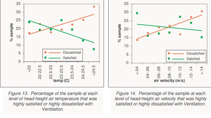
Obviously, air temperature (RTD_H) is associated with ventilation satisfaction in general, and thermal comfort in particular [Charles, 2003], and the result of our analysis is shown in Figure 13. Over a wider range of temperatures, one would expect a quadratic relationship, with lower

satisfaction for temperatures that are either too hot or too cold. However, over the range of temperatures we observed, linear fits work best, with lower temperatures generally perceived as more satisfactory than higher temperatures. The crossover point in our analysis is ~22.5 - 23 oC. Interestingly, this is similar to the predicted neutral temperature from Fanger’s thermal comfort equation, which is the foundation of the most widely used thermal comfort standards [ASHRAE, 1992; ISO, 1994]. Putting in the mean observed values for relative humidity (30%)

and air velocity (0.09 ms-1), assuming a typical sedentary activity (1.2 met), and a light office clothing ensemble (0.8 clo insulation), and the common assumption that radiant temperature

equals air temperature, Fanger’s equation yields4 a neutral temperature of 23.2 oC. Air velocity (AIR_V_H) was also significantly correlated with SatVent votes in our field study

regressions. It is possible that air velocity that is too low or too high could be perceived negatively. For the data we had, a linear fit works best, particularly for the Highly Dissatisfied

group (see Figure 14). The crossover point is ~0.1 ms-1, with air velocities higher than this perceived negatively. This might mean that higher air velocities are perceived as draughty. Current recommendations [e.g., ASHRAE, 1992, BCBC, 1997] suggest that air velocity should

not exceed 0.15 – 0.25 ms-1 in office spaces.

The regressions on field study data indicate no statistically significant relationship between relative humidity and SatVent ratings. Thermal comfort research does indicate an effect of humidity, but it might be that the relative humidities measured in this field study (M=30%, s.d.=11%) were too low and in too small a range to have much of an effect. As the COPE

software doesn’t calculate humidity, we did not pursue this relationship further. The field study regressions do show a significant effect of proximity to a window on SatVent ratings. People with windows in their cubicles had significantly lower ratings, and the principal

explanation was probably lower temperatures [Newsham et al., 2003]. However, all of our measurements were made during Winter or Spring, and it is possible that temperatures close to windows would be higher at other times of the year. The COPE software does not include seasonal variations, and so we chose not to pursue the relationship between Satisfaction with

Ventilation and window proximity any further.

The normal state for ventilation control in open-plan offices is central control with (ideally for the system design) identical flow rates out of each supply diffuser. Studies show that individual ventilation control is associated with improved satisfaction [Charles, 2002]. In such cases individual control included a supply diffuser dedicated to an individual workstation with

control over one or more of: direction, flow rate, and temperature. Individual control also reduces complaints and delivers energy savings [Pero, 2002]. Therefore, the algorithm

Individual Control

Absent

0 5 10 15 20 25 30 35 40 45 <4 8 48-54 54-60 60-66 66-72 >7 2 min PH % sam p le Satisfied Dissatisfied

Figure 11. Percentage of the sample at each level of minimum partition ht. that was highly satisfied or highly dissatisfied with Ventilation.

Linear fits to the data points are also shown.

0 5 10 15 20 25 30 35 40 < 500 500-550 550-600 600-650 650-700 700-750 750-800 > 800 CO2 (ppm) % sam p le Satisfied Dissatisfied

Figure 12. Percentage of the sample at each level of carbon-dioxide concentration that was

highly satisfied or highly dissatisfied with Ventilation. 0 5 10 15 20 25 30 35 <2 2 22 -22. 5 22 .5-23 23 -23. 5 23 .5-24 24 -24. 5 > 24. 5 temp (C) % sam p le Satisfied Dissatisfied

Figure 13. Percentage of the sample at each level of head-height air temperature that was

highly satisfied or highly dissatisfied with Ventilation. 0 5 10 15 20 25 30 35 <. 0 4 .04-.06 .06-.08 .08-.10 .10-.12 .12-.14 >. 1 4 air velocity (m/s) % sam p le Satisfied Dissatisfied

Figure 14. Percentage of the sample at each level of head-height air velocity that was highly

4.0 Discussion

So far in this report we have used the word algorithms to describe the range of each physical condition that predicts a positive or negative effect on satisfaction. This is to be consistent with

the terminology in software, where these ‘algorithms’ will be used, and with the terminology used in previous COPE discussions and documents. According to the Oxford English Dictionary on-line, the definition of an algorithm is ‘a process, or set of rules, usually one expressed in algebraic notation’. Another word to describe what has been developed in this report would be heuristics. To paraphrase the dictionary definition of heuristics, they are ‘rules that might guide decisions, but that are not foolproof’5. We used a process to derive each rule

that was founded on one or more of the following three conditions, each of them perfectly valid:

• statistically significant regressions from our field study data;

• statistically significant relationships from other work in the literature; • widely accepted and published recommended practice.

The method we used, looking at the differences in physical conditions between Highly Satisfied and Highly Dissatisfied groups, agreed with expected trends and yielded reasonable

results, though there is clearly a degree of uncertainty in where the crossover points are defined. Nevertheless, this method is arguably as valid as prevailing methods for developing

published recommended practices.

There are other issues to be mindful of when applying these rules to predict satisfaction in offices. Remember that the critical values for each physical parameter were identified using the point at which membership in the Highly Satisfied group was more likely than membership

in the Highly Dissatisfied group. However, the Highly Dissatisfied population did not drop to zero for any physical parameter over the ranges we studied. This means that designing in the

directions suggested by the heuristics does not guarantee a workplace free from indoor environment complaints. The best way to think of the accumulation of results from the heuristics is as an overall expression of risks to the satisfaction of a population of office workers exposed to the conditions, rather than as a deterministic prediction of absolute

satisfaction ratings for an individual.

An extension of this is that no one satisfaction negative (

"

!

indoor environment, we suggest taking remedial action only for designs associated with a multitude of satisfaction negatives.

Another important point is that the positives and negatives are not necessarily equal in their expected effect on overall environmental satisfaction. An individual positive or negative

expresses a potential satisfaction effect of one particular physical variable, it cannot necessarily be equated to a positive or negative related to a different physical variable. The corollary of this is that positives and negatives cannot be meaningfully traded off against each

other. That is, a design that generates a total of four negatives and two positives (

""""

!!

""

two of the positives cancel out two of the negatives to leave two negatives) or a design rated as

"""

!

5

For example, the Oxford English Dictionary Online [OED] references the following definition of heuristic as a noun: 1957 A. NEWELL et al. in Proc. Western Joint Computer Conf. XV. 223 A process that may solve a given problem, but offers no guarantees of doing so, is called a heuristic for that problem.

The issue of the relative weight accorded to each satisfaction effect is one that could be tackled in future research. “Combined effects” have been studied to a limited extent in previous research [Nelson et al., 1994; Veitch, 1990; Hygge, 1991; Alm et al., 1999; Witterseh

et al., 1999; Hygge and Knez, 2001], but have looked at only a narrow range of the physical parameters explored in this report. It would also be valuable to confirm the value of the heuristics we have developed in a laboratory experiment where extraneous variables can be

controlled. One could begin by comparing, in a human factors experiment, an office design that would be assigned a large number of negatives in our current heuristics, with a design that

would be assigned a large number of positives.

Despite the informal nature of their development, we believe these heuristics offer a useful beginning for the global characterization of environmental satisfaction in offices. There is no doubt that that they need future validation and extension. We hope they will act as a spur to

the further development of guidelines for office environments founded on occupant satisfaction.

5.0 References

Alm, O., Witterseh, T., Clausen, G., Toftum, J. & Fanger, P. O. (1999). “The impact on human perception of simultaneous exposure to thermal load, low-frequency ventilation noise and indoor air pollution”. Proceedings of Indoor Air ’99: the 8th International Conference on Indoor

Air Quality and Climate (Edinburgh, Scotland) 5, pp. 270-275.

ASHRAE. American Society of Heating, Refrigerating, and Air-Conditioning Engineers. (1992). Thermal environmental conditions for human occupancy (ANSI/ASHRAE Standard 55).

Atlanta, GA: ASHRAE.

ASHRAE. American Society of Heating, Refrigerating, and Air-Conditioning Engineers. (2001). Ventilation for acceptable indoor air quality (ASHRAE Standard 62). Atlanta, GA: ASHRAE. Benya, J.; Heschong, L.; McGowan, T.; Miller, N.; Rubinstein, F. (2001). Advanced Lighting

Guidelines. New Buildings Institute, WA, USA.

Berrutto, V.; Fontoynont, M.; Avouac-Bastie, P. (1997). “Importance of wall luminance on users satisfaction: pilot study on 73 office workers”, Proceedings of Lux Europa (Amsterdam)

8th European Lighting Conference, pp. 82-101.

Boubekri, M. and Haghighat, F. (1993). “Windows and environmental satisfaction: a survey study of an office building”, Indoor Environment, 2, pp. 164-172.

Boyce, P.R.; Eklund, N.H.; Simpson, S.N. (2002). “Individual lighting control: task performance, mood, and illuminance”, Journal of the Illuminating Engineering Society of North

America, Winter, pp. 131-142.

Bradley, J.S. (2003). “The acoustical design of conventional open plan offices”, Canadian Acoustics, 31(2), pp. 23-30.

Bradley, J.S. and Gover, B.N. (2003). “Describing Levels of Speech Privacy in Open-Plan Offices”, IRC Client Report B3144.8.

Brill, M., Margulis, S. T., Konar., E., & BOSTI. (1984). Using office design to increase productivity. Buffalo, N.Y. Workplace Design and Productivity, Inc.

BCBC. British Columbia Buildings Corporation. (1997). Technical standards. BCBC. Charles, K.E.; Veitch, J.A.; Farley, K.M.J.; Newsham, G.R. (2003). “Environmental Satisfaction in Open-Plan Environments: 3. Further Scale Validation”. IRC Internal Report

IR-152.

Charles, K.E. (2002). “Office Air Distribution Systems and Environmental Satisfaction”. IRC Research Report RR-161.

Charles, K.E.; Veitch, J.A. (2002). “A Literature Review on the Relationship between Outdoor Ventilation Rates in Offices and Occupant Satisfaction”. IRC Research Report RR-160. Charles, K.E. (2003). “Fanger’s Thermal Comfort and Draught Models”. IRC Research

Report RR-162.

Christoffersen, J.; Johnsen, K.; Petersen, E.; Valbjorn, O.; Hygge, S. (2000). “Windows and daylight - a post-occupancy evaluation of Danish offices”, Proceedings of CIBSE/ILE Joint

Lighting Conference (York, UK), pp. 112-120.

CIBSE. (1993). Lighting for Offices. The Chartered Institute of Building Services Engineers, London, UK.

Duval, C.L.; Charles, K.E.; Veitch, J.A. (2002). “Open-Plan Office Density and Environmental Satisfaction”. IRC Research Report RR-150.

Finnegan, M.C.; Solomon, L.Z. (1981). “Work attitudes in windowed vs. windowless environments”, The Journal of Social Psychology, 115, pp. 291-292.

Hygge, S. (1991). “The interaction of noise and mild heat on cognitive performance and serial reaction time”. Environment International, 17, pp. 229-234.

Hygge, S. & Knez, I. (2001). “Effects of noise, heat and indoor lighting on cognitive performance and self-reported affect”. Journal of Environmental Psychology, 21, pp. 291-299.

IESNA. (2000). Handbook of the Illuminating Engineering Society of North America, 9th Edition (Ed. Rea, M.S). Illuminating Engineering Society of North America, New York, USA.

ISO. International Standards Organization. (1994). Moderate thermal environments: Determination of the PMV and PPD indices and specification of the conditions for thermal

comfort (ISO 7730). Geneve, Switzerland: ISO.

Jennings, J.D.; Rubinstein, F.M.; DiBartolomeo, D.; Blanc, S.L. (2000). “Comparison of control options in private offices in an advanced lighting controls testbed”, Journal of the

Illuminating Engineering Society of North America, Summer, pp. 39-60.

Jones, C.C.; Richman, E.; Heerwagen, J.; Reinertson, J.; McKay, H. (1998). Federal Lighting Guidelines. US Department of Energy, Washington DC.

Leather, P.; Pyrgas, M.; Beale, D.; Lawrence, C. (1998). “Windows in the workplace: sunlight, view, and occupational stress”, Environment and Behavior, 30(6), pp. 739-762.

Loe, D. L.; Mansfield, K. P.; Rowlands, E. (1994). “Appearance of lit environment and its relevance in lighting design: experimental study”, Lighting Research and Technology 26(3), pp.

119 – 133.

Lorusso, T.P.; Hedge, A.; Middendorf, S. (2001). “Do anti-glare filters help computer users in offices?”, Proceedings of the Human Factors and Ergonomics Society 45th Annual Meeting

(Minneapolis), pp. 786-790.

Moore, T.; Carter, D.J.; Slater, A. I. (2002). "A study of occupant controlled lighting in offices ", Lighting Research and Technology, 34(3), pp. 191-205.

Maniccia, D.; Rutledge, B.; Rea, M.S.; Morrow, W. (1999). “Occupant use of manual lighting controls in private offices”, Journal of the Illuminating Engineering Society of North America,

Summer, pp. 42-56.

Marquardt, C.J.G.; Veitch, J.A.; Charles, K.E. (2002). “Environmental satisfaction with open-plan office furniture design and layout”. IRC Research Report RR-106.

Muramatsu, R.; Nakamura, Y. (2002). “Evaluation of lighting environment using conjoint analysis (part 1) - for the case of office”, Journal of Light & Visual Environment, 26(3),

pp.30-39.

Navai, M. and Veitch, J.A. (2003). “Acoustic Satisfaction in Open plan Offices: Review and Recommendations”. IRC Research Report RR-151.

Nelson, T. M., Nilsson, T. H. & Johnson, M. (1984). “Interaction of temperature, illuminance and apparent time on sedentary work fatigue”. Ergonomics, 27(1), pp. 89-101.

Newsham, G.R., Sander D.M. (2002). “The effect of office design on workstation lighting: a simulation study”, Proceedings of the IESNA Annual Conference (Salt Lake City), pp. 399-424

(also available as “The Effect of Office Design on Workstation Lighting: Simulation Results”. IRC Internal Report IR-847).

Newsham, G.R.; Veitch, J.A. (2001). "Lighting quality recommendations for VDT offices: a new method of derivation," Lighting Research and Technology, 33, (2), pp. 97-116. Newsham, G.R.; Marchand, R.G., Veitch, J.A. (2004). “Preferred Surface Luminances in Offices, by Evolution”, Journal of the Illuminating Engineering Society of North America, 33(1),

Winter, pp. 14-29.

Newsham, G.R.; Veitch, J.A.; Charles, K.E.; Bradley, J.S.; Shaw, C.Y.; Reardon, J.T.; Marquardt, C.; J.G. Geerts, J. (2003). “Environmental Satisfaction in Open-Plan Environments: 4. Relationships Between Physical Variables”. IRC Research Report RR-153.

OED. Oxford English Dictionary Online, Oxford University Press, http://dictionary.oed.com/entrance.dtl/

Oldham, G. R. (1988). “Effects of changes in workspace partitions and spatial density on employee reactions: A quasi-experiment”, Journal of Applied Psychology, 73(2), pp. 253-258. Oldham, G. R., & Fried, Y. (1987). “Employee reactions to workspace characteristics”, Journal

of Applied Psychology, 72(1), pp. 75-80.

Pero, K. (2002). Private communication on 1 Front Street Building renovations by Public Works and Government Services Canada.

Reinhart, C.F. (2002). “Effects of interior design on the daylight availability in open plan offices”, Conference Proceedings of the 2002 Summer Study of the American Commission for

an Energy Efficient Environment (ACEEE), (Pacific Grove, CA), pp. 1-12.

Seppanen, O.A.; Fisk, W.J.; Mendell, M.J. (1999). “Association of ventilation rates and CO2 concentrations with health and other responses in commercial and institutional buildings”,

Indoor Environment, 9, pp. 226-252.

Shaw, C.Y., MacDonald, R.A., Galasiu, A.D., Reardon, J.T., Won, D.Y. (2003). “Experimental Investigation of Ventilation Performance in a Mock-up Open-plan Office”, pp. 46. IRC Client

Report B-3205.19.

Shaw, C.Y., J.S. Zhang, M.N. Said, F.Vaculik, and R.J. Magee. (1993). “Effect of Air Diffuser Layout on the Ventilation Conditions of a Workstation: Part II - Air Change Efficiency and

Ventilation Efficiency”, ASHRAE Transactions, 99(2).

Slater, A. I.; Boyce, P. R. (1990). "Illuminance Uniformity on Desks: Where is the Limit?," Lighting Research and Technology, 22(4), pp. 165-174.

USGBC. United States Green Building Council, LEED (Leadership in Energy and Environmental Design) Green Building Rating System™

http://www.usgbc.org/LEED/LEED_main.asp

Veitch, J. A. (1990). “Office noise and illumination effects on reading comprehension”. Journal of Environmental Psychology, 10, pp. 209-217.

Veitch, J. A.; Newsham, G. R. (1998). "Lighting quality and energy-efficiency effects on task performance, mood, health, satisfaction and comfort," Journal of the Illuminating Engineering Society, 27(1), Winter, pp. 107-129 (Also presented at the Illuminating Engineering Society of

North America Annual Conference (Seattle, WA), 1997.)

Veitch, J. A.; Newsham, G. R. (2000). “Exercised Control, Lighting Choices, and Energy Use: An Office Simulation Experiment”, Journal of Environmental Psychology, 20, pp.

219-237.

Veitch, J.A., Farley, K.M.J., Newsham, G.R. (2002a). “Environmental Satisfaction in Open-Plan Environments: 1. Scale Validation and Methods”. 63rd Annual Convention of the Canadian Psychological Association (Vancouver, B.C) (also available as IRC Internal Report

No. 844).

Veitch, J.A., Bradley, J.S., Legault, L.M., Norcross, S., Svec, J.M. (2002b). “Masking Speech in Open-Plan Offices with Simulated Ventilation Noise: Noise Level and Spectral Composition

Effects on Acoustic Satisfaction”. IRC Internal Report IR-846.

Veitch, J.A., Charles, K.E, Newsham, G.R., Marquardt, C.J.G., Geerts, J. (2003). Environmental Satisfaction in Open-Plan Environments: 5. Workstation and Physical Condition

Effects”. IRC Research Report RR-154.

Wilkins, A. J.; Nimmo-Smith, I.; Slater A.; Bedocs, L. (1989). “Fluorescent lighting, headaches and eyestrain”, Lighting Research and Technology, 21, pp. 11-18.

Witterseh, T., Wargocki, P, Fang, L., Clausen, G. & Fanger, P. O. (1999). “Effects of exposure to noise and indoor air pollution on human perception and symptoms”. Proc. of Indoor Air99:

6.0 Acknowledgements

This investigation forms part of the Field Study sub-task for the NRC/IRC project Cost-effective Open-Plan Environments (COPE) (NRCC Project # B3205), supported by Public Works and Government Services Canada, Natural Resources Canada, the Building Technology Transfer

Forum, Ontario Realty Corp, British Columbia Buildings Corp, USG Corp, and Steelcase, Inc. COPE is a multi-disciplinary project directed towards the development of a decision tool for the

design, furnishing, and operation of open-plan offices that are satisfactory to occupants, energy-efficient, and cost-effective. Information about the project is available at http://irc.nrc-cnrc.gc.ca/ie/cope. We are grateful to contributions of the entire COPE team, whose work on