Monitoring and predicting SARS-CoV-2 epidemic in France after deconfinement using a multiscale age-dependent rate model

HAL Id: hal-02585716

https://hal.archives-ouvertes.fr/hal-02585716v2

HAL is a multi-disciplinary open access

archive for the deposit and dissemination of sci-entific research documents, whether they are pub-lished or not. The documents may come from teaching and research institutions in France or abroad, or from public or private research centers.

L’archive ouverte pluridisciplinaire HAL, est destinée au dépôt et à la diffusion de documents scientifiques de niveau recherche, publiés ou non, émanant des établissements d’enseignement et de recherche français ou étrangers, des laboratoires publics ou privés.

Monitoring and predicting SARS-CoV-2 epidemic in

France after deconfinement using a multiscale

age-dependent rate model

Jürgen Reingruber, Andrea Papale, David Holcman

To cite this version:

Jürgen Reingruber, Andrea Papale, David Holcman. Monitoring and predicting SARS-CoV-2 epidemic in France after deconfinement using a multiscale age-dependent rate model. 2020. �hal-02585716v2�

Monitoring and predicting SARS-CoV-2 epidemic in France after

deconfinement using a multiscale age-dependent rate model

J¨urgen Reingruber, Andrea Papale, David Holcman Group of data modeling and computational biology, IBENS-PSL Ecole Normale Superieure, Paris, France. ∗

May 17, 2020

Abstract

The entire world and France were strongly impacted by the SARS-COV-2 epidemic. Finding appropriate measures that effectively contain the spread of the epidemic without putting a too severe pressure on social and economic life is a major challenge for modern predictive approaches. To assess the impact of confinement (March 17th till May 11th) and deconfinement, we develop a novel rate model to monitor and predict the spread of the epidemic and its impact on the health care system. The model accounts for age-dependent interactions between population groups and predicts consequences for various infection categories such as number of infected, hospitalized, load of intensive care units (ICU), number of death, recovered from hospitalization and more. We use online health care data for the five most infected regions of France to calibrate the model. At day of deconfinement (May 11th), we find that 13% (around 4.8M) of the population is infected in the five most affected regions of France (extrapolating to 5.8M for France). The model predicts that if the reproduction number R0is reduced by at least a factor of 2.5-3 for all age groups after

deconfinement, which could be achieved by wearing masks and social distancing, a significant second peak can be prevented. However, if the reduction in R0 for the age group 0-25 would be

less and below 2 (e.g. due to school openings), a second peak with ICU saturation is unavoidable. In that context, we argue that testing should be focused on children, but without tracing it will nevertheless have only a very limited impact on reducing the spread.

1

Introduction

The fast spreading worldwide pandemic of SARS-CoV-2 has destabilized all major economies of the world in only a few months, forcing most European countries into confinement. This measure has curbed in few days the disease progression. To prepare the deconfinement and to recover economical prosperity, most of the affected western countries rely on the efficiency of wearing masks and on social distancing, hoping that these measures will be sufficient to prevent a second peak of infection that could saturate hospitals and ICU. For such fast spreading and severe pandemic [1], predictive modeling is crucial to estimate in advance the impact of deconfinement measures, because small deviations can rapidly be exponentially amplified [2, 3, 4, 5]. Yet predicting with high accuracy remains a major challenge during this crisis [6, 7].

Very quickly after the beginning of the pandemic, public web sites have provided daily data for hospitalizations, ICU occupancy, deaths, recovered, etc.., which is crucial to obtain an age-stratified

∗

analysis [8]. The large number of severe cases in particular for the age groups 60-69 and older than 70 has destabilized the ICUs. But this data alone provides only a partial understanding of the mechanisms that govern the pandemic social propagation. It remains challenging to reconstruct the pandemic dynamics from this live data for several reasons: incomplete data, change in social interactions, or unknown fraction of the population that are asymptomatic, which are not accounted for in public health data.

In order to understand the dynamics of SARS-CoV-2 transmission and to predict the infection spread and the status of the health care system after deconfinement, we develop a discrete dynamical model that we implement for 5 different age groups (group 1=0-24, group 2=25-49, group 3=50-59, group 4=60-69, and group 5=70+) and 8 different infection categories (Tables S2 and S3). Because the distribution of infected in the 5 most affected regions (ˆIle de France, Grand Est, Auvergne Rhˆone Alpes, Hauts-de-France and Provence-Alpes-Cˆote d’Azur) and the rest of France is very heterogeneous (the 5 regions together concentrate 36.9M people (67M for France) but account for 80% of the reported cases), we focused on these 5 regions to calibrate and validate the model, and to test several scenarios for the time after deconfinement. We found that the number of infected after lockdown is 13% (around 4.8M) in the five most affected regions and 5.8M of the total French population, in line with a recent report emphasizing the large number of asymptomatic in the population (15.5% from [9]) and slightly higher than a recent estimation of 3.7M infected [10]. Because of this low fraction of infected, a second catastrophic peak after deconfinement is unavoidable without proper control and social distancing measures. We found that wearing masks for the entire population could be a means to steadily prevent a second peak without the need of going through several re- and deconfinement phases. Moreover, we show that school opening poses a serious risk that could destabilize the deconfinement phase if social distancing measures and wearing of masks are not rigorously followed. If testing capacities are limited, we propose to focus testing on children to timely unravel the asymptomatic infected. However, we also find that testing without tracing only has a very limited effect on containing the pandemic.

2

Results

The distribution of hospitalizations from public data reveals a strong heterogeneity of the infection spread throughout France (Fig. 1A-B). We therefore focused our analysis on data from the 5 most affected regions, which represent around 54% of the French population (36.7M) and around 80% of the reported cases. The age resolved time series for the number of hospitalizations, ICU occupancy, cumulative returned from hospital and cumulative deceased are very similar between the 5 regions and the entire country (Fig. 1D-E), and the ratio of these numbers is almost constant (Fig. 1F). Thus, our results and predictions for the 5 regions can be extrapolated to entire France by multiplying with a factor around 1.2 instead of a factor around 2 corresponding to the population ratio.

2.1 Model calibration with public data

The present model accounts for 5 different age groups (group 1=0-24, group 2=25-49, group 3=50-59, group 4=60-69, and group 5=70+) and 8 different infection categories (Tables S3 and S2). The model has a time resolution of one day and uses switching probabilities to compute the daily time evolution (see Methods). Parameters can be updated at any day to incorporate modified conditions (e.g. lockdown or hospitalisation procedures).

To account for social interactions before confinement, we use the contact matrix between age groups in France from [13]. Since before lockdown we did not have access to age stratified data,

All 0-24: group 1 25-49: group 2 50-59: group 3 60-69: group 4 >70: group 5 Age groups 5 Regions Île-de-France Grand-Est Auvergne-Rhône-Alpes Hauts-de-France Provence-Alpes-Côte d'Azur

(A)Number of hospitalized people _{France 5 regions Ratio}

(B) (D) (E) (F) (1) (2) (4) (1) (2) (3) (4) (1) (2) (3) (4) (C)

Admitted people in ICU per day

(3)

Time since 18/03/2020 [days] Time since 18/03/2020 [days] Time since 18/03/2020 [days] France: 23 921 5 regions: 19 187 Île-de-France Grand-Est Auvergne-Rhône-Alpes Provence-Alpes-Côte d'Azur Hauts-de-France Occitanie Bourgogne-Franche-Comté Centre-Val de Loire Normandie Nouvelle-Aquitaine 0 10 20 30 40 50 1.05 1.10 1.15 1.20 1.25 1.300 10 20 30 40 50 1.10 1.15 1.20 1.25 1.30 1.35 1.40 1.450 10 20 30 40 50 1.1 1.2 1.3 1.4 1.50 10 20 30 40 50 1.05 1.10 1.15 1.20 1.25 1.30 1.35 0 10 20 30 40 50 0 2000 4000 6000 8000 10 000 0 10 20 30 40 50 0 5000 10 000 15 000 0 10 20 30 40 50 0 500 1000 1500 0 10 20 30 40 50 0 2000 4000 6000 8000 10 000 12 000 14 000 0 10 20 30 40 50 0 2000 4000 6000 8000 10 000 12 000 0 10 20 30 40 50 0 5000 10 000 15 000 20 000 0 10 20 30 40 50 0 500 1000 1500 2000 0 10 20 30 40 50 0 5000 10 000 15 000 20 000 Ho sp ita lized IC U Re tur ne d H om e De ath s

Figure 1: Public French health care data. (A) Map of France emphasizing the 5 most in-fected regions at 6th of May: ˆIle de France, Grand Est, Auvergne Rhˆone Alpes, Hauts-de-France and Provence-Alpes-Cˆote d’Azur. (B) Distribution of people in ICU. (C) 5 Regions and age group stratification. (D-E) Age resolved time series for hospitalized (1), ICU occupancy (2), cumulated recovered from hospitalization (3) and cumulated deaths (4) for France and the 5 regions. (F) Ratio between the data in D (entire France) and E (5 regions). The color code for the age groups is defined in panel C. Data source [11, 12].

we only calibrated the exponential growth rate for the number of new infections (0.18day−1, see Fig. S1) by modifying the infectiousness parameter β (see Eq. 6 in the Methods; the infectiousness is independent of age [14]). Using β and the contact matrix from [13] we found for the time before confinement for the five groups the reproduction numbers [3.8, 3.1, 2.7, 2.4, 0.5] (see Eq. 7 in the Methods). The reproduction numbers are different for each group because of the internal structure of the contact matrix. For the averaged collective reproduction number, we obtain ¯R0 = 2.5 (see

Eq. 8). If we account only for the young and active population (groups 1-3) that make most of the social contacts, we get ¯R0 = 3.2, similar to [10, 15]. To conclude, to accurately monitor the pandemic

one has to consider age dependent reproduction numbers.

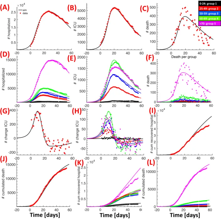
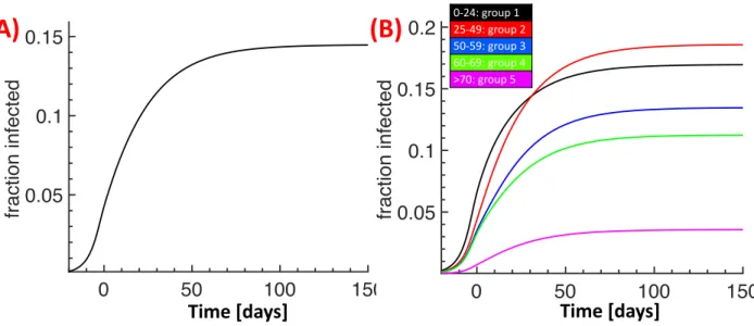
After lockdown, we used the age-stratified public data for the 5 regions [11, 12] for model cal-ibration. We changed the contact matrix to account for the reduction in social interactions (see Methods). We then tuned our model parameters (e.g. probability to become hospitalized, probabil-ity to develop severe symptoms, decease probabilities etc) to obtain simultaneous agreement between all the available data and the model predictions (Fig. 2). Interestingly, the very different behaviour of the hospitalization data for group 5 could only be accounted for by increasing the duration of hos-pitalization over time, which probably reflects change in the policy of hoshos-pitalization for this group (personal communication). Although the model predictions for group 5 for number of hospitaliza-tions, cumulated death and ICU occupancy match very well with the data (magenta curves in Fig. 2 D,E,L), the model overestimates the number of recovered for this group model (Fig. 2 K) starting around day 20 after lockdown. The exact reason is unclear, a possible explanation could be that the number of interactions for group 5 further decreased during lockdown. At the end of the confinement period, the model predicts that around 13% of the population has been infected (Fig. 3A), most of them in group 1 and 2 (Fig. 3B). Finally, due to the reduced social interactions, the reproduction numbers for the five groups after lockdown are reduced to [0.73, 1.08, 0.74, 0.67, 0.25]. The collective reproduction number is ¯R0 = 0.69, which is around a factor of 4 smaller compared to pre-lockdown.

To conclude, the calibrated and validated model precisely reproduces the available data, and can now be used to study in detail the pandemic progression and its load on the health care system after deconfinement.

2.2 Prediction of the pandemic without lockdown

We used the calibrated model to show the drastic consequences for the hypothetical case that the lockdown would not have happened (Fig. 4). In the absence of confinement, we predict a total of 250,000 deaths in the 5 regions (Fig. 4D), which would extrapolate to ∼450,000 deaths in France. In this uncontrolled case the majority of the population would become infected (around 87%, Fig. 4A), and the ICU would remain saturated for around 50 days (Fig. 4C). Age stratified simulation results for this scenario are shown in Fig. S2.

2.3 Prediction of the pandemic with full deconfinement and absence of social restrictions

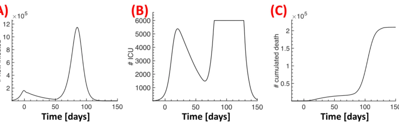
If all social restrictions would be alleviated after deconfinement, we predict a large second peak for the new infections (around 6 times the first one) that would occur around mid-July (Fig. 5A) with around 220,000 cumulated deaths for the 5 regions at the end (Fig. 5C). ICU would be saturated for 50 days (Fig. 5B), with a need 320,000 hospitalizations at the peak (Fig. S3B).

-20 0 20 40 60 -200 0 200 400 # change ICU -20 0 20 40 60 5000 10000 15000 # cumulated death -20 0 20 40 60 0.5 1 1.5 2 2.5

# cum recovered hospital

104 -20 0 20 40 60 1 2 3 4 5 6

# cum recovered hospital

104 -20 0 20 40 60 0 100 200 300 400 # death

Death per group

-20 0 20 40 60 100 200 300 400 500 # death -20 0 20 40 60 5000 10000 15000 # hospitalized -20 0 20 40 60 500 1000 1500 2000 # ICU 0-24: group 1 25-49: group 2 50-59: group 3 60-69: group 4 >70: group 5 -20 0 20 40 60 -50 0 50 100 150 # change ICU

Time [days]

Time [days]

Time [days]

(J)

_(K)

(G)

(H)

(I)

(E)

(F)

(B)

(D)

(C)

(A)

(L)

Figure 2: Calibration of the model using age-stratified data for the 5 regions after lockdown. We compare data (diamonds) with simulation results (continuous lines). Total number of hospitalized (A), ICU occupancy (B), daily deaths (C) and their age group distributions (respectively D, E and F); daily variation of people in ICU (G) and its age group distribution (H); cumulative number of people recovered from hospitalization (I) and cumulative number of deaths in hospitals (J) and their age group distributions (respectively K and L). Day zero corresponds to the 18th of March.

Time [days]

Time [days]

0

50

100

150

0.05

0.1

0.15

fraction infected

0

50

100

150

0.05

0.1

0.15

0.2

fraction infected

(A)

(B)

Figure 3: Fraction of infected without deconfinement. Fraction of the infected population for the 5 regions (A) and its age group distribution (B).

Time [days]

Time [days]

(A)

(B)

(C)

(D)

Figure 4: Pandemic spread in absence of lockdown. The figure shows the drastic consequences for the hypothetical case that the lockdown would not have been imposed. Continuous lines show simulation results, the red dots are the data from Fig. 2. New infections (A), hospitalizations (B), ICU occupancy (C) and cumulative deaths (D).

Time [days] Time [days] 0 Time [days]50 100 150 0.5 1 1.5 2 # cumulated death 105 0 50 100 150 1000 2000 3000 4000 5000 6000 # ICU 0 50 100 150 2 4 6 8 10 12 # new infected 105

(A)

(B)

(C)

Figure 5: Full deconfinement without social restrictions. Simulation results for the case that all social restrictions would be alleviated after deconfinement. New infections (A), ICU occupancy (B) and cumulative deaths (C).

2.4 Controlling the pandemic by wearing masks

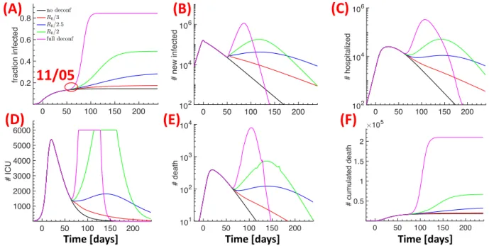
Several evidences suggest that wearing a mask could efficiently attenuate the epidemic spread [16] by reducing the propagation of viral particles due to breathing, coughing or sneezing, as revealed by a recent analysis using Laser Light Scattering [17]. However, as demonstrated in the case of influenza virus, coarse and fine droplets with diameters > 5µm and < 5µm are not reduced by the same proportion by wearing masks. Whereas course droplets are reduced by a factor of 25, fine droplets are reduced only by a factor of 2.8 [18]. Since fine droplets contain around ten times more viral particles than course droplets, and they stay much longer in the respiratory environment [18], we hypothesize that wearing masks could reduce the infectiousness by a similar factor. We thus explored how the pandemic would spread if the social interactions after deconfinement would be the same as before lockdown, but wearing of masks would reduce the infectiousness β, and thus the reproduction number ¯R0. In Fig. 6 we tested three scenario where ¯R0 is reduced by a factor of 3 (strict mask

wearing, red curves), 2.5 (less strict, blue curves) and 2 (insufficient, green curves). For comparison, we also show the results for the no-deconfinement scenario (black curves) and the scenario with full deconfinement (magenta curves). The cumulated number of deaths for the 5 regions is 21,000 (R0/3), 35,000 (R0/2.5 and 70,000(R0/2) (Fig. 6F) with 16%, 30% and 50% of the population infected

(Fig. 6A) .

Next we explored the consequences that children under 11 are not obliged to wear masks at school. We assume that adults (group 2 -5) strictly wear their masks resulting in a reduction of their infectiousness by a factor of 3, whereas the reduction for group 1 is only by a factor of 2 (Fig. 7, red curves) or 1.5 (Fig. 7, blue curves). We found that with a reduction by a factor of 2 the deconfinement phase remains under control with no large second peak and ICUs remain unsaturated (Fig. 7A-D, red curves). However, by only slightly increasing R0 for group 1 by a factor of 1.33 a large second

peak emerges (Fig. 7A-D, blue curves). The number of hospitalized would reach 540,000 beginning of August, ICU would start to be saturated around beginning of July and the cumulated number of deceased would reach around 60,000 (around 3 times the level of end of April in the 5 regions). This suggests that the behaviour of group1 could destabilize the deconfinement phase if not carefully controlled.

Finally, we explored whether testing could reduce the second peak for the case that the infec-tiousness of group2 is only reduced by a factor of 1.5 (Fig. 7A-D, green curves). We assume that 100,000 tests can be made every day, and an infected person that has been tested it is removed from

the pool of infectious the day after testing. Because the infectious population in group 1 generates the second peak, simulations (not shown) reveal that focusing all the testing capacities on group 1 is most effective. However, even in this case (green curves in Fig. 7) the second peak would only be slightly reduced and the health care system would still be destabilized with 50,000 deceased people after 150 days post confinement (mid-August).

We conclude that whereas wearing masks efficiently is key to keep the pandemic under control, testing without tracing has only a very limited impact. In addition, it is problematic to trace children that usually have no smartphones. Thus, school openings without efficient control can destabilize the deconfinement phase.

Time [days] Time [days] 0 50Time [days]100 150 200

0.5 1 1.5 2 # cumulated death 105 0 50 100 150 200 101 102 103 104 # death 0 50 100 150 200 102 104 106 # hospitalized 0 50 100 150 200 1000 2000 3000 4000 5000 6000 # ICU 0 50 100 150 200 0.2 0.4 0.6 0.8 fraction infected 0 50 100 150 200 102 104 106 # new infected

(A)

(B)

(D)

(E)

(C)

(F)

11/05

Figure 6: Effect of wearing masks after deconfinement. Wearing masks corresponds to a reduction in infectiousness and the reproduction number R0. Comparison of three scenarios where

R0 is reduced by 3 (strict mask wearing, red curves), 2.5 (less strict, blue curves) and 2 (insufficient, green curves). The results for no deconfinement (black curves) and full deconfinement with no restrictions (magenta curves) are also shown for comparison. Fraction of infected people (A), daily new infected (B), hospitalized people (C), ICU occupancy (D), daily deaths (E), and cumulative number of deceased (F).

3

Discussion

Preventing the natural exponential spread of the pandemic is a major challenge of the deconfinement phase. Using public health care data we developed a novel age-stratified modeling approach that combines social interaction matrices with dynamical modeling to reproduce and predict the time course of the pandemic spread and its consequences for the health care system. A major strength of our approach is to simultaneously account for a variety of different age stratified data such as hospitalization, ICU occupancy, recovered from hospitalization, which provides strong confidence for the model predictions.

0 50 100 150 200 1 2 3 4 5 6 # cumulated death 104 gp1 3 gp1 2 gp1 1.5 gp1 1.5+test 0 50 100 150 200 1000 2000 3000 4000 5000 6000

# ICU

Time [days]

Time [days]

(A)

(C)

(D)

(B)

Figure 7: Possible effect of school openings after deconfinement. Comparison of four scenarios for the time after deconfinement where the infectiousness for group 2-4 is reduced by 3, whereas for group 1 it is reduced by a factor of 3 ( black curves, corresponding to the red curves in Fig. 6), 2 (red curves) and 1.5 (blue curves). In the forth scenario we added testing for group 1 (green curves). New daily infected (A), hospitalized (B), ICU occupancy (C), cumulative number of deaths (D).

exp(βt) of confirmed cases and number of death from β = 0.2 (Fig. S1) to β = 0.004 (Table S5), which confirmed the immediate effect of the lockdown on the exponential spread of the pandemic. Since the number of susceptible after lockdown is still very high, and asymptomatic persons are difficult to reveal, it remains a major challenge to avoid a return to an exponential growth phase with similar rates as before lockdown. Our detailed causal dynamical model allows to explore the time evolution of the pandemic for various scenarios, and thus provides a tool to refine and adapt political decisions. By continuously adapting the model parameters to real time data, simulations can be used to predict the evolution of the pandemic in order to test and implement in advance efficient social measures to control and contain the pandemic spread.

In the absence of social measures a catastrophic second wave is unavoidable [10, 15, 2], however, we found that wearing masks for the entire population could prevent this to happen without the need to go through several re- and deconfinement phases. In that context, we find that school openings without rigorous control of wearing masks and social distancing measures poses a serious risk to destabilize the deconfinement phase. If testing capacities are limited, we further argue that the focus should be on testing school children to timely unravel the asymptomatic infected. However, we also show that testing without tracing only has a limited effect on containing the pandemic.

Supplementary Information

Methods

Model description

We developed a discrete switching model with a single day as unit timestep. Although we imple-mented the model for 5 age groups and 7 infection categories (Tables S2 and S3), the model structure is general such that a higher degree of diversifications can be implemented without problems. For example, an advanced version of the model could include more age groups, and the groups could be further divided according to female and male. A major problem was to derive a consistent initial parametrization that is compatible with all the available data and disease properties from the liter-ature. However, once such an initial parametrization is obtained, it is a much easier task to adapt the model parameters to a more diversified version of model.

The model variables are:

• S(n|k): Number of susceptible persons at day n belonging to group k.

• I(n, m, l|k, j): Number of infected persons belonging to group k, infection category j, day m after infection and day l after switching to infection category j.

• Iinf(n, m, l|k, j) = ξ(m, l|k, j)I(n, m, l|k, j): Number of infectious.

• Inew(n|k): Number of new infected.

• D(n, m, l|k, j) = a(m, l|k, j)I(n, m, l|k, j): Number of deceased.

• R(n, m, l|k, j) = p(n, m, l|k, j, J_max)(I(n, m, l|k, j) − D(n, m, l|k, j)): Number of recovered.

The algorithm for the time evolution with Σ(n, m, l|k, j) = I(n, m, l|k, j) − D(n, m, l|k, j) is

S(n + 1|k) = S(n|k) − Inew(n|k) I(n + 1, 1, 1|k, 1) = Inew(n|k) I(n + 1, m + 1, l + 1|k, j) = p(n, m, l|k, j, j)Σ(n, m, l|k, j) I(n + 1, m + 1, 1|k, j) = X l,j0_6=j p(n, m, l|k, j0, j)Σ(n, m, l|k, j0) . (1)

The switching probabilities p(n, m, l|k, J0, J ) can be time dependent and satisfy the normalization P

Jp(n, m, l|k, J

0_{, J ) = 1. With the cumulative number of dead and recovered persons per group}

Dcum(n|k) = X n0_,m,l,j D(n0, m, l|k, j) Rcum(n|k) = X n0_,m,l,j R(n0, m, l|k, j) . (2)

we obtain the conservation equation

S(n + 1|k) + Itot(n + 1|k) + Rcum(n|k) + Dcum(n|k) = (3)

New infections

To estimate the number of new infections we consider the number of contacts c(n|k, k0) that group k and k0 make at day n. The total number of contacts group k make is c(n|k) =P

k0c(n|k, k0). The

number of infectious persons in group k is

Iinf(n|k) =

X

m,l,j

ξ(m, l|k, j)I(n, m, l|k, j) , (4)

where ξ(m, l|k, j) is a projection operator that selects infectious out of infected persons. We consider that only asymptomatic persons are infectious between 5 − 11 days after infection (incubation time is 5 days), and infected persons that show symptoms put themselves in quarantine. The amount of new infections in group k generated by infectious in group k0 is

Inew(n|k, k0) = βk0S(n|k) Pk c(n|k, k0)Iinf(n|k 0₎ Pk0 , (5)

where Pk is the population in group k, and βk the infectiousness of group k. The total number of

new infected in group k is

Inew(n|k) = X k0 βk0S(n|k) Pk Iinf(n|k0) Pk0 c(n|k, k 0_{) . (6)}

The parameter βk describes the infectiousness per group (can be time dependent), and for example

depends on the fraction of people that wear masks in group k. Because there is no solid evidence that the infectiousness changes with age, we assume for the initial pandemic phase and also for the lockdown phase (since masks were largely unavailable) that βk= β is the same for all groups. After

deconfinement we use a group dependent βk to implement the possibility that the fraction of people

that wear masks varies between groups.

Reproduction numbers

To connect β to reproduction numbers, we consider the initial condition with S(1|k)_P

k = 1 and a single

infectious person in group i, Iinf(1|k) = δk,i. The total number of infected generated by this person

per day is X k Inew(1|k) = β X k c(1|i, k) Pi = βc(1|i) Pi = ˜R0,i, (7)

where ˜R0,i is the reproduction number per day. Eq. 7 shows that if the number of contacts is

proportional to the group size, c(1|k)_Pk = const, then ˜R0,k is the same for all groups. Moreover, Eq. 7

together with Eq. 5 reveal that the number of new infected is does not change if the normalization of the contact matrix is altered.

To connect ˜R0,k defined per day to the classical reproduction number ¯R0, we consider that an

infected person is infectious for in average ¯dk days. The mean reproduction number per infections

period is then ¯R0,k = ˜R0,kd¯k , and the averaged collective reproduction number is

¯ R0 = 1 ngp X k ¯ R0,k = 1 ngp X k ˜ R0,kd¯k, (8)

where ngp= 5 is the number of groups.

An infected person can start to develop symptoms between days 6 − 10 with overall probability Pk(Qk= 1 − Pk is the probability of remaining asymptomatic), in which case he is put in quarantine

the next day. With this information, the mean number of days an infected person remains infectious is ¯ dk= 2 + Pk 1 − pk pk (9) where pk = 1 − (1 − Pk) 1

ds _{and ds= 5. The factor of 2 in Eq. 9 accounts for the fact that a person}

that starts to show symptoms is removed from the pool of infectious only the following day. With 20% asymptomatic for group 1-3 and 10% for group 4-5 we get ¯dk= [4.1, 4.1, 4.1, 3.5, 3.5].

Contact matrix

The contact matrix before lockdown for our group definitions is obtained from the frequency matrix in [13] (S3 Table Base-case contact matrix with age categories for all contact and for skin contact only) by summing over the corresponding age groups. The resulting normalized contact matrix is

        gp1 gp2 gp3 gp4 gp5 gp1 0.7564 0.2565 0.0652 0.0385 0.0125 gp2 0.2565 0.4818 0.1367 0.0967 0.0283 gp3 0.0652 0.1367 0.0840 0.0479 0.0120 gp4 0.0385 0.0967 0.0479 0.0689 0.0274 gp5 0.0125 0.0283 0.0120 0.0274 0.0140         (10)

To estimate the reduced contact matrix after lockdown we used the following reduction matrix:

        gp1 gp2 gp3 gp4 gp5 gp1 0.20 0.25 0 0 0 gp2 0.25 0.40 0.40 0.25 0.5 gp3 0 0.40 0.40 0 0.5 gp4 0 0.25 0 0.65 0.3 gp5 0 0.50 0.50 0.30 1         (11)

To build the reduction matrix, we made several ad hoc assumptions motivated by the following arguments: the intra-group contacts for group 1 are mostly redundant and therefore strongly reduced by 80%. The inter-group contact between group 1 and group 2 corresponds to parents children interactions, which is reduced to 25% of the original contacts. In contrast, we assume that the contacts made by group 5 are mostly important and therefore cannot be as strongly reduced as for group 1. We assume no contacts between group 1 and 5 (complete disruption of the relation with grand-children), however, we kept the contact with the other groups due to social needs. Finally, We fine tuned these values to fit the hospitalized data.

Code availability

Parameter Description

n Time in days

m Number of days after infection

l Number of days in an infection category.

k Group index.

1 ≤ j ≤ jmax Infection category. Monitors disease progression.

1 ≤ J ≤ jmax+ 1 Infection category with recovered category.

a(m, l|k, j) Probability to die. Infected only die in category 5 and 6. p(n, m, l|k, Jold, Jnew) Probability to switch from category Jold to Jnew.

P

Jnewp(n, m, l|k, Jold, Jnew) = 1 (normalization)

p(n, m, l|k, Jmax, Jmax) = 1 (no switching from recovered category)

c(n|k, k0) Contact matrix.

ξ(m, l|k, j) Matrix to identify infectious persons. Only asymptomatic are infections during 5 − 11 days after infection.

Pk Population in group k.

βk Infectiousness of group k.

Table S1: Parameter definitions,

k Group Population (37M) 1 0-24 10.1M (30%) 2 25-49 12.1M (33%) 3 50-59 4.7M (13%) 4 60-69 3.6M (10%) 5 70+ 5.5M (15%)

Table S2: Population groups for the five regions. Source:

https://www.statista.com/statistics/464032/distribution-population-age-group-france/

J, j Category of infected persons J, j = 1 Asymptomatic

J, j = 2 With symptoms

J, j = 3 Hospitalized with mild symptoms J, j = 4 Hospitalized with severe symptoms

J, j = 5 Hospitalized with severe symptoms and ICU necessity. Persons in this category are automatically transferred to category 6 if ICU is available.

J, j = 6 ICU

J, j = 7 Hospitalized after ICU, or after ICU necessity J = 8 Recovered

Author contributions

JR conceived the model, performed analysis and implemented the model in MATLAB. DH and JR refined and further developed the model and calibrated the model to data. AP and DH collected and analysed data. All authors contributed to writing of the manuscript.

Competing interests

The authors declare no competing interests.

Acknowledgement

A. P. received funding from FRM (SPF201909009284), D. H. is supported by INSERM Plan Cancer and a Computational Neuroscience NIH-ANR grant. J. R. is supported by an ANR grant. We thanks Pr. Dan Longrois for some discussions about ICU’s organization.

Data for different countries

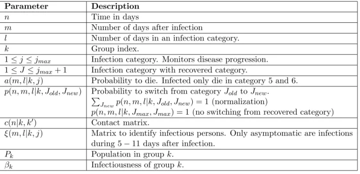
Data plotted in figure S1 are taken from the repository managed by John Hopkins University https: //github.com/CSSEGISandData/COVID-19. Four different countries have been considered: France, Italy, Germany and Czech Republic. Discontinuities in data are related to detection methods of each country. Curves are fitted using an exponential function, f (t) = α · eβ·t+ γ (dashed lines in the figure). Fits have been performed before lockdown (17th March (France), 9th March (Italy), 22nd March (Germany) and 18th March (Czech Republic)) using Mathematica software, results are reported in the table.

France Italy Germany Czech Republic

Confirmed 0.18 ± 0.02 0.19 ± 0.01 0.25 ± 0.01 0.26 ± 0.01 Deaths 0.18 ± 0.03 0.27 ± 0.01 0.36 ± 0.02 xxx

Table S4: Fit exponents β before confinement

France Italy Germany Czech Republic

Confirmed 0.004 ± 0.001 0.003 ± 0.001 0.003 ± 0.001 0.003 ± 0.001 Deaths 0.005 ± 0.001 0.002 ± 0.001 0.09 ± 0.01 0.09 ± 0.01

Table S5: Fitted exponents β in the first period after confinement. Fits after lockdown are performed using ten points (last point 10th April).

Hospitalization data

Data related to the hospitals after the lockdown have been provided by French Government www. data.gouv.fr are reported in figure 1. In particular our analysis is based on the data in the following databases: donnees-hospitalieres-covid19 and donnees-hospitalieres-classe-age-covid19. The first one contains the number of hospitalized people, currently in critical care (ICU), returned home and deaths divided for departments, the second the same data divided for regions and the relative age group distribution. In particular we focus our analysis on the most affected french regions: ˆIle de France, Grand Est, Auvergne Rhˆone Alpes, Hauts-de-France and Provence-Alpes-Cˆote d’Azur. The age group distributions are available since the 18th of March (30 April is missing).

Supplementary figures

Time since lockdown

Death s (No rmal ized ) Czech Republic France Germany Italy 𝑓(𝑡)~𝑒!" 𝑓(𝑡)~𝑒!"

Time since lockdown [time]

N

orm

al

iz

ed

c

on

firm

ed

c

as

es

N

orm

al

iz

ed

de

aths

Time since lockdown [time]

-30 -20 -10 0 10 20 30 40 0.001 0.010 0.100 1 10 100 1000

Time since lockdown

Co n fi rmed cases (No rmal ized ) 𝜷 = 𝟎. 𝟏𝟖 ± 𝟎. 𝟎𝟐 𝜷 = 𝟎. 𝟏𝟗 ± 𝟎. 𝟎𝟏 𝜷 = 𝟎. 𝟐𝟓 ± 𝟎. 𝟎𝟏 𝜷 = 𝟎. 𝟐𝟔 ± 𝟎. 𝟎𝟐 𝜷 = 𝟎. 𝟏𝟖 ± 𝟎. 𝟎𝟑 𝜷 = 𝟎. 𝟐𝟕 ± 𝟎. 𝟎𝟏 𝜷 = 𝟎. 𝟑𝟔 ± 𝟎. 𝟎𝟏 𝜷 = 𝟎. 𝟐𝟖 ± 𝟎. 𝟎𝟒

(A)

(B)

Figure S1: Exponential rates of confirmed cases (A) and deaths (B) before lockdown for Czech Republic, France, Germany and Italy. Data are rescaled with values at the beginning of lockdown. Since the number of deaths for Czech Republic on 18th March was zero, the curve in panel (B) is scaled to one.

-20 0 20 40 60 80 100 0 1 2 3 4 5 10 5 Hospitalized -20 0 20 40 60 80 100 0 1 2 3 4 10 5 Hospitalized -20 0 20 40 60 80 100 -1 -0.5 0 0.5 1 1.5 2 10 4 Change in hospitalization -20 0 20 40 60 80 100 0 1000 2000 3000 4000 5000 6000 ICU -20 0 20 40 60 80 100 0 500 1000 1500 2000 2500 3000 ICU -20 0 20 40 60 80 100 -600 -400 -200 0 200 400 Change in ICU -20 0 20 40 60 80 100 0 0.5 1 1.5 2 2.5 10 5 Cumulated death -20 0 20 40 60 80 100 0 5 10 15 104 Cumulated death -20 0 20 40 60 80 100 0 2000 4000 6000 8000 Death -20 0 20 40 60 80 100 0 2 4 6 8 10 5Cumulated recovered -20 0 20 40 60 80 100 0 1 2 3 4 5 10 5Cumulated recovered -20 0 20 40 60 80 100 0 2000 4000 6000 8000 10000 Recovered 0-24: group 1 25-49: group 2 50-59: group 3 60-69: group 4 >70: group 5

(A)

(B)

(C)

(D)

(E)

(F)

(G)

(H)

(I)

Time [days] Time [days] Time [days]

Prediction of health care saturation in absence of confinement

(J)

(K)

(L)

Figure S2: Prediction of pandemic spread and health care evolution in the absence of lockdown. Total number of hospitalized people (A), its age group distribution (B) and the daily variations (C); people in ICU (D), age group distribution in ICU (E) and the daily variations (F); cumulated deaths (G), age group distribution (H) and daily death (I); cumulative number of people recovered from hospitalization (J), age group distribution (K) and daily variations (L). Continuous lines show simulation results, dashed lines the actual data.

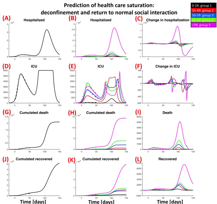
0 50 100 150 0 1 2 3 4 10 5 Hospitalized 0 50 100 150 0 0.5 1 1.5 2 2.5 3 10 5 Hospitalized 0 50 100 150 -1 -0.5 0 0.5 1 1.5 10 4 Change in hospitalization 0 50 100 150 0 1000 2000 3000 4000 5000 6000 ICU 0 50 100 150 0 500 1000 1500 2000 2500 3000 ICU 0 50 100 150 -600 -400 -200 0 200 400 Change in ICU 0 50 100 150 0 0.5 1 1.5 2 2.5 10 5 Cumulated death 0 50 100 150 0 5 10 15 10 4 Cumulated death 0 50 100 150 0 1000 2000 3000 4000 5000 6000 Death 0 50 100 150 0 1 2 3 4 5 6 105Cumulated recovered 0 50 100 150 0 1 2 3 4 10 5Cumulated recovered 0 50 100 150 -2000 0 2000 4000 6000 8000 10000 Recovered

Prediction of health care saturation:

deconfinement and return to normal social interaction

0-24: group 1 25-49: group 2 50-59: group 3 60-69: group 4 >70: group 5

(A)

(B)

(C)

(D)

(E)

(F)

(G)

(H)

(I)

(J)

(K)

(L)

Time [days] Time [days] Time [days]

Figure S3: Prediction of pandemic spreading and health care saturation with full decon-finement and return to social interactions as before lockdown. Total number of hospitalized people (A), its age group distribution (B) and the daily variations (C); people in ICU (D), age group distribution in ICU (E) and the daily variations (F); cumulated deaths (G), age group distribution (H) and daily death (I); cumulative number of people recovered from hospitalization (J), age group distribution (K) and daily variations (L). Continuous lines show simulation results, dashed lines the actual data.

0 50 100 150 0 0.5 1 1.5 2 2.5 3 10 4 Hospitalized 0 50 100 150 0 5000 10000 15000 Hospitalized 0 50 100 150 -500 0 500 1000 Change in hospitalization 0 50 100 150 0 1000 2000 3000 4000 5000 6000 ICU 0 50 100 150 0 500 1000 1500 2000 ICU 0 50 100 150 -100 -50 0 50 100 150 Change in ICU 0 50 100 150 0 0.5 1 1.5 2 10 4 Cumulated death 0 50 100 150 0 5000 10000 15000 Cumulated death 0 50 100 150 -100 0 100 200 300 400 500 Death 0 50 100 150 0 2 4 6 8 10 10 4Cumulated recovered 0 50 100 150 0 1 2 3 4 5 10 4Cumulated recovered 0 50 100 150 -200 0 200 400 600 800 Recovered

Prediction of health care saturation:

deconfinement and social measure to keep R0/3

0-24: group 1 25-49: group 2 50-59: group 3 60-69: group 4 >70: group 5

Time [days] Time [days] Time [days]

(A)

(B)

(C)

(D)

(E)

(F)

(G)

(H)

(I)

(J)

_(K)

(L)

Figure S4: Predictions of health care evolution in a scenario with deconfinement and R0

reduced by a factor of 3 compared to pre-lockdown. Total number of hospitalized people (A), its age group distribution (B) and the daily variations (C); people in ICU (D), age group distribution in ICU (E) and the daily variations (F); cumulated deaths (G), age group distribution (H) and daily death (I); cumulative number of people recovered from hospitalization (J), age group distribution (K) and daily variations (L). Continuous lines show simulation results, dashed lines the actual data.

0 50 100 150 200 0 0.5 1 1.5 2 2.5 3 10 4 Hospitalized 0 50 100 150 200 0 5000 10000 15000 Hospitalized 0 50 100 150 200 -500 0 500 1000 Change in hospitalization 0 50 100 150 200 0 1000 2000 3000 4000 5000 6000 ICU 0 50 100 150 200 500 1000 1500 ICU 0 50 100 150 200 -100 -50 0 50 100 150 Change in ICU 0 50 100 150 200 0 1 2 3 4 10 4 Cumulated death 0 50 100 150 200 0 0.5 1 1.5 2 2.5 3 10 4 Cumulated death 0 50 100 150 200 -100 0 100 200 300 400 500 Death 0 50 100 150 200 0 5 10 15 10 4 Cumulated recovered 0 50 100 150 200 0 2 4 6 8 10 4 Cumulated recovered 0 50 100 150 200 -200 0 200 400 600 800 Recovered 0-24: group 1 25-49: group 2 50-59: group 3 60-69: group 4 >70: group 5

(A)

(B)

(C)

(D)

(E)

(F)

(G)

(H)

(I)

(J)

(K)

(L)

Prediction of health care saturation:

deconfinement and social measure to keep R0/2.5

Time [days] Time [days] Time [days]

Figure S5: Predictions of health care evolution in a scenario with deconfinement and R0 reduced by a factor of 2.5 comapred to pre-lockdown. Total number of hospitalized

people (A), its age group distribution (B) and the daily variations (C); people in ICU (D), age group distribution in ICU (E) and the daily variations (F); cumulated deaths (G), age group distribution (H) and daily death (I); cumulative number of people recovered from hospitalization (J), age group distribution (K) and daily variations (L). Continuous lines show simulation results, dashed lines the actual data.

References

[1] R. Verity, L. C. Okell, I. Dorigatti, P. Winskill, C. Whittaker, N. Imai, G. Cuomo-Dannenburg, H. Thompson, P. G. T. Walker, H. Fu, A. Dighe, J. T. Griffin, M. Baguelin, S. Bhatia, A. Boonyasiri, A. Cori, Z. Cucunub´a, R. FitzJohn, K. Gaythorpe, W. Green, A. Hamlet, W. Hinsley, D. Laydon, G. Nedjati-Gilani, S. Riley, S. [van Elsland], E. Volz, H. Wang, Y. Wang, X. Xi, C. A. Donnelly, A. C. Ghani, and N. M. Ferguson, “Estimates of the severity of coron-avirus disease 2019: a model-based analysis,” The Lancet Infectious Diseases, 2020.

[2] N. M. Ferguson, D. Laydon, G. Nedjati-Gilani, N. Imai, K. Ainslie, M. Baguelin, S. Bha-tia, A. Boonyasiri, Z. Cucunub´a, G. Cuomo-Dannenburg, A. Dighe, I. Dorigatti, H. Fu, K. Gaythorpe, W. Green, A. Hamlet, W. Hinsley, L. C Okell, S. van Elsland, H. Thompson, R. Verity, E. Volz, H. Wang, Y. Wang, P. G. Walker, C. Walters, P. Winskill, C. Whittaker, C. A. Donnelly, S. Riley, and A. C. Ghani, “Report 9: Impact of non-pharmaceutical inter-ventions (npis) to reduce covid-19 mortality and healthcare demand,” Imperial College London, 2020.

[3] J. Dehning, J. Zierenberg, F. P. Spitzner, M. Wibral, J. P. Neto, M. Wilczek, and V. Priesemann, “Inferring change points in the covid-19 spreading reveals the effectiveness of interventions,” Apr 2020.

[4] F. Balabdaoui and D. Mohr, “Age-stratified model of the covid-19 epidemic to analyze the impact of relaxing lockdown measures: nowcasting and forecasting for switzerland,” medRxiv, 2020.

[5] M. J. Keeling, E. Hill, E. Gorsich, B. Penman, G. Guyver-Fletcher, A. Holmes, T. Leng, H. McKimm, M. Tamborrino, L. Dyson, and M. Tildesley, “Predictions of covid-19 dynam-ics in the uk: short-term forecasting and analysis of potential exit strategies,” medRxiv, 2020.

[6] N. P. Jewell, J. A. Lewnard, and B. L. Jewell, “Caution warranted: Using the institute for health metrics and evaluation model for predicting the course of the covid-19 pandemic,” Annals of internal medicine, pp. M20–1565, 04 2020.

[7] I. for Health Metrics and Evaluation, “New covid-19 forecasts: Us hospitals could be over-whelmed in the second week of april by demand for icu beds, and us deaths could total 81,000 by july,” 2020.

[8] WorldHealthOrganization, “Population-based age-stratified seroepidemiological investigation protocol for covid-19 virus infection,” 2020.

[9] H. Streeck, B. Schulte, B. Kuemmerer, E. Richter, T. Hoeller, C. Fuhrmann, E. Bartok, R. Dolscheid, M. Berger, L. Wessendorf, M. Eschbach-Bludau, A. Kellings, A. Schwaiger, M. Co-enen, P. Hoffmann, M. Noethen, A.-M. Eis-Huebinger, M. Exner, R. Schmithausen, M. Schmid, and B. Kuemmerer, “Infection fatality rate of sars-cov-2 infection in a german community with a super-spreading event,” medRxiv, 2020.

[10] H. Salje, C. Tran Kiem, N. Lefrancq, N. Courtejoie, P. Bosetti, J. Paireau, A. Andronico, N. Hoze, J. Richet, C.-L. Dubost, Y. Le Strat, J. Lessler, D. L. Bruhl, A. Fontanet, L. Opatowski, P.-Y. Bo¨elle, and S. Cauchemez, “Estimating the burden of SARS-CoV-2 in France.” working paper or preprint, Apr. 2020.

[11] “https://geodes.santepubliquefrance.fr/.”

[12] “https://www.data.gouv.fr/fr/datasets/donnees-hospitalieres-relatives-a-lepidemie-de-covid-19.”

[13] G. B´eraud, S. Kazmercziak, P. Beutels, D. Levy-Bruhl, X. Lenne, N. Mielcarek, Y. Yazdanpanah, P.-Y. Bo¨elle, N. Hens, and B. Dervaux, “The french connection: The first large population-based contact survey in france relevant for the spread of infectious diseases,” PLOS ONE, vol. 10, pp. 1–22, 07 2015.

[14] T. Jones, B. M¨uhlemann, T. Veith, M. Zuchowski, J. Hofmann, A. Stein, A. Edelmann, V. Max Corman, and C. Drosten, “An analysis of sars-cov-2 viral load by patient age,” Preprint, 2020.

[15] L. Di Domenico, G. Pullano, C. E. Sabbatini, Bo¨elle, Pierre-Yves, and V. Colizza, “Report 9, expected impact of lockdown in ˆıle-de-france and possible exit strategies,” 2020.

[16] K. K. Cheng, T. H. Lam, and C. C. Leung, “Wearing face masks in the community during the covid-19 pandemic: altruism and solidarity,” The Lancet, 2020.

[17] P. Anfinrud, V. Stadnytskyi, C. E. Bax, and A. Bax, “Visualizing speech-generated oral fluid droplets with laser light scattering,” New England Journal of Medicine, 2020.

[18] D. K. Milton, M. P. Fabian, B. J. Cowling, M. L. Grantham, and J. J. McDevitt, “Influenza virus aerosols in human exhaled breath: Particle size, culturability, and effect of surgical masks,” PLOS Pathogens, vol. 9, pp. 1–7, 03 2013.