Particle identification of neutral particles at LHCb

PoS(LHCP2018)046

LPC, Clermont-Ferrand, France

E-mail:boris.quintana@cern.ch

Important analyses of the core LHCb physics program rely on calorimetry to identify photons, high-energy neutral pions and electrons. For this purpose, the LHCb calorimeter system is composed of a scintillating pad plane, a preshower detector, an electromagnetic and a hadronic sampling calorimeters. The interaction of a given particle in these detectors leaves a specific signature. This is exploited for particle identification (PID) by combining calorimeters and tracking information into multivariate classifiers.

In this contribution, we focus on the identification of photons against high-energy neutral pions, electrons and hadronic backgrounds. Neutral particles reconstruction process at LHCb is succinctly explained and PID performances on Run 1 data is shown. Discrepancies with simulation predictions are then discussed, with special emphasis on the methods to correctly estimate PID cut efficiencies by means of large calibration samples of abundant beauty and charm decays to final states with photons or π0. Finally, the technical aspects of the collection of these samples in Run 2 are presented.

Sixth Annual Conference on Large Hadron Collider Physics (LHCP2018) 4-9 June 2018

Bologna, Italy

∗_Speaker.

PoS(LHCP2018)046

The ability to identify the nature of particles is one of the major requirements in a flavor physics experiment. At LHCb, one challenging feature is the identification of neutrals. Important analyses of the core LHCb physics program rely on calorimetry to identify photons, high-energy neutral pions and electrons. For instance, a good γ/π0 separation is an important prerequisite for the study of radiative decays such as Bs→ φ γ, B0→ K∗γ , B±→ φ K±γ and Λb→ Λ0γ , to reject π0 background contributions. Besides, this can be useful in the opposite case, rejecting photons when studying B decay modes with a π0in the final state, as in Bs→ KKπ0and Bs→ Kππ0.

2. Reconstruction of neutral particles

The calorimeter system of LHCb [1] is composed of a Scintillating Pad Detector (SPD), a Preshower (PS), an Electromagnetic Calorimeter (ECAL) and a Hadronic Calorimeter (HCAL). The ECAL is based on the Shashlik technology and contains 6016 cells. In front of the ECAL, the PS is composed of 6016 tiles matching the geometry of the ECAL. The PS is placed after a lead sheet of 2.5 radiation length and is preceded by another layer of 6016 scintillator tiles, the SPD. The energy deposits of different particles in the calorimeters are displayed on Figure1.

Figure 1: Energy deposited on the different parts of the calorimeter system by an electron, a hadron, and a photon

The reconstruction of electromagnetic showers process starts with the identification of the ECAL cell that has an excess in energy deposition, referred to as local maximum or seed cell, com-pared to all its direct neighbours (3-9 cells). These cells are selected only if the transverse energy is larger than 50 MeV. The identified cell will originate a cluster according to the clusterisation procedure adopted by the Cellular Automaton algorithm [2]. The selection of neutral clusters is performed using an anti-matching technique with reconstructed tracks : reconstructed tracks in the event are extrapolated to the calorimeter and then all-to-all matching with the reconstructed clusters is performed.

Around 88% of the photons detected by the calorimeter originate from π0decays. The signa-ture in the ECAL depends on its kinematics, the higher the momentum of the π0 is the closer the two photons are at the entry of the calorimeter. These two photons can then either produce two separated clusters or share a single cluster in which their individual signals are not clearly distin-guishable.

PoS(LHCP2018)046

which the transverse momentum spectrum starts around 2 GeV/c. To reconstruct resolved π0, pho-tons are paired and their invariant mass, mγ γ, is compared with the π0mass : mγ γ is required to be in the range 105 to 165 MeV/c2. To reconstruct merged π0, each electromagnetic cluster is split in two subclusters defined from the two most energetic cells in the cluster. After the preparation of the two photon subclusters, a specific creteria relying on the energy in the cluster and the reconstructed merged π0mass is applied to identify the cluster as coming from a π0. In 70% of cases, a merged π0 can be misidentified as a single photon. Actually, the dominant background of the radiative decays corresponds to merged π0_{, which amounts up to 50-60% of the background. Therefore the} use of an efficient PID variable is crucial.

3. Multivariate approaches to PID

Particle identification (PID) algorithms are based on multivariate classifiers. They combine informations from different subdetectors, such as variables describing the track-cluster matching, or the shape of the neutral cluster, into a discriminant output. They are trained to separate photons signatures from hadrons and electrons, which may have passed the neutral cluster selection, and high-energy π0.

Three different Neural Networks (MultiLayer Perceptrons - MLP) are trained using Monte Carlo simulation of either non-electromagnetic particles, electrons from B → K∗eesimulation, or decays with a π0such as B0→ K+_π−

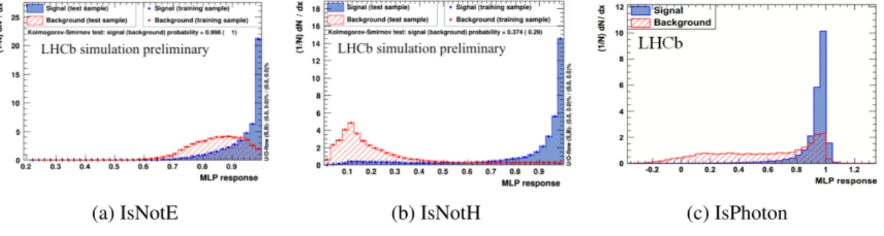
π0, and where the hadron/electron/π0is reconstructed as a photon. The three corresponding output variables are named respectively IsNotH, IsNotE and IsPhoton [3]. The PID variables distributions for both signal(true photons) and background(h/e/π0) are displayed on Figure2.

(a) IsNotE (b) IsNotH (c) IsPhoton

Figure 2: Output distributions of the neutral PID Neural Networks IsNotE, IsNotH and IsPhoton. Due to MC/data discrepancies in the input variables used to build the γ /π0separation variable, discrepancies are also expected in the output of the method. It can be seen on Figure3where the photon efficiency versus π0rejection for both data and MC is shown.

In order to get a true estimate of the selection efficiency for a given cut on the IsPhoton variable, calibration samples from real data are needed.

PoS(LHCP2018)046

In order to calibrate the performance of the IsPhoton variable, B0→ K∗

γ reconstructed events are used as a calibration sample for photons and D0→ Kππ0 _{events selected from D}∗+_{→ D}0

π+ for merged π0.

For the Run 1, B0→ K∗γ sample takes into account the whole B0→ K∗γ data collected by the LHCb detector over the 2011-2012 period accounting for 3 fb−1of integrated luminosity. The D0→ Kππ0 sample is obtained only using 2011 data. It has been selected from D∗+→ D0

π+with a very tight mass cut |MD∗+− M_D0|, hence resulting in a very clean sample. In order to extract pure samples to use for the calibration, the invariant mass distribution is modeled and the sPlot technique [4] is then used to extract weights for the signal component so as to have background subtracted samples.

Figure 3: Photon selection efficiency as a function of π0 rejection for data and MC simulation.

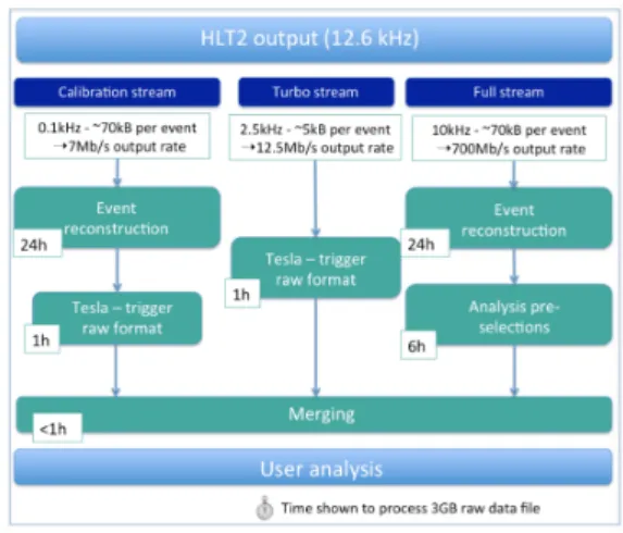
Figure 4: Workflow of the Calibration stream for Run 2.

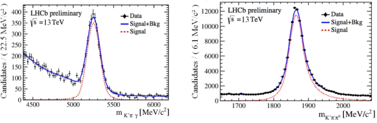
For the Run 2, thanks to the real-time detector alignment and calibration, selected exclusive decays with both online (Turbo) and offline (Full) informations are available directly at the second High Level Trigger (HLT 2) with the TurCal stream (Turbo - Calibration [5], Figure4). This feature allows to select bigger calibration samples with respect to Run 1, improving also the phase-space coverage adding new decay modes (Table1). The preliminary mass fits for the B0 → K∗

γ and D0→ Kππ0_{Run2 samples are shown in Figure5.}

γ calibration modes π0calibration modes D+→ (η0→ π+

π−γ )π+ B→ K∗γ D∗+(2010) → (D0→ K−π+π0)π+(π0resolved) D∗+_s → (D+

s → K+K−π+)γ Bs→ φ γ D∗+(2010) → (D0→ K−π+π0)π+(π0merged) Table 1: Run 2 calibration modes for γ and π0.

PoS(LHCP2018)046

computed in each bins of variables that are correlated with the PID (e.g. ET, pseudo-rapidity). The MC samples can then either be reweighted to match the PID selected data, or resampled to correct the distribution of the PID variable.

Figure 5: Fits to the B and D0invariant mass in B → K∗γ (left) and D0→ Kππ0(right) calibration samples.

5. Conclusion

The separation between neutral particles signatures in the calorimeters is achieved with multi-variate classifiers, using discriminant informations from the LHCb calorimeter sub-detectors, and gives good performances. However, as the simulated samples used for the Neural Network training does not represent the real data with full accuracy, discrepancies in the tools performance between data and MC are expected. From this comes the need for large samples of calibration data, to get a true estimate of PID requirements. While these samples are provided for photons and π0through a dedicated offline selection process for the Run 1, the Turbo-Calib stream implemented for the Run 2 allows a much more convenient online selection of large calibration samples. A dedicated tool is available to analysts to correct the γ/π0separation variable (IsPhoton) distribution in MC simulated samples, and work is on-going to propose a similar tool for the two others neutral PID variables. References

[1] R. Aaij et al. [LHCb Collaboration], LHCb Detector Performance, Int. J. Mod. Phys. A 30 (2015) no.07, 1530022 [arXiv:1412.6352 [hep-ex]].

[2] V. Breton, N. Brun and P. Perret, A clustering algorithm for the LHCb electromagnetic calorimeter using a cellular automaton, LHCb-2001-123, CERN-LHCb-2001-123.

[3] M. Calvo Gomez et al., A tool for γ/π0_{separation at high energies Tech. Rep. 2252}

LHCb-PUB-2015-016.

[4] M. Pivk and F. R. Le Diberder, SPlot: A Statistical tool to unfold data distributions, Nucl. Instrum. Meth.A 555 (2005) 356 [physics/0402083 [physics.data-an]].

[5] R. Aaij et al. [LHCb Collaboration], Tesla : an application for real-time data analysis in High Energy