RESEARCH OUTPUTS / RÉSULTATS DE RECHERCHE
Author(s) - Auteur(s) :
Publication date - Date de publication :
Permanent link - Permalien :
Rights / License - Licence de droit d’auteur :
Dépôt Institutionnel - Portail de la Recherche
researchportal.unamur.be
University of Namur
Reduced point charge models of proteins: Assessment based on molecular dynamics simulations Leherte, Laurence Published in: Molecular Simulation DOI: 10.1080/08927022.2015.1044452 Publication date: 2016 Document Version
Peer reviewed version
Link to publication
Citation for pulished version (HARVARD):
Leherte, L 2016, 'Reduced point charge models of proteins: Assessment based on molecular dynamics
simulations', Molecular Simulation, vol. 42, no. 4, pp. 289-304. https://doi.org/10.1080/08927022.2015.1044452
General rights
Copyright and moral rights for the publications made accessible in the public portal are retained by the authors and/or other copyright owners and it is a condition of accessing publications that users recognise and abide by the legal requirements associated with these rights. • Users may download and print one copy of any publication from the public portal for the purpose of private study or research. • You may not further distribute the material or use it for any profit-making activity or commercial gain
• You may freely distribute the URL identifying the publication in the public portal ?
Take down policy
If you believe that this document breaches copyright please contact us providing details, and we will remove access to the work immediately and investigate your claim.
For Peer Review Only
Reduced point charge models of proteins: Assessment based on molecular dynamics simulations
Journal: Molecular Simulation/Journal of Experimental Nanoscience Manuscript ID: GMOS-2014-0417.R1
Journal: Molecular Simulation Date Submitted by the Author: n/a
Complete List of Authors: Leherte, Laurence; University of Namur, Chemistry
Keywords: molecular electrostatic potential, smoothing of molecular fields, reduced point charge model, Ubiquitin, Barnase–Barstar
For Peer Review Only
Reduced point charge models of proteins: Assessment based on
molecular dynamics simulations
Laurence LEHERTE
Laboratoire de Physico-Chimie Informatique Unité de Chimie Physique Théorique et Structurale Department of Chemistry
Namur MEdicine & Drug Innovation Center (NAMEDIC)
University of Namur, Rue de Bruxelles 61, B-5000 Namur (Belgium)
[email protected] Tel. +32-81-72.45.60 3 4 5 6 7 8 9 10 11 12 13 14 15 16 17 18 19 20 21 22 23 24 25 26 27 28 29 30 31 32 33 34 35 36 37 38 39 40 41 42 43 44 45 46 47 48 49 50 51 52 53 54 55 56 57 58 59 60
For Peer Review Only
Reduced point charge models of proteins: Assessment based on
molecular dynamics simulations
A reduced point charge distribution is used to model Ubiquitin and two complexes, Vps27 UIM-1–Ubiquitin and Barnase–Barstar. It is designed from local extrema in charge density distributions obtained from the Poisson equation applied to smoothed molecular electrostatic potentials. A variant distribution is built by locating point charges on atoms. Various charge fitting conditions are selected, i.e., from either electrostatic Amber99 Coulomb potential or forces, considering reference grid points located within various distances from the protein atoms, with or without separate treatment of main and side chain charges. The program GROMACS is used to generate Amber99SB molecular dynamics (MD) trajectories of the solvated proteins modelled using the various reduced point charge models (RPCM) so obtained. Point charges that are not located on atoms are considered as virtual sites. Some RPCMs lead to stable MD
trajectories. They however involve a partial loss in the protein secondary structure and lead to a less structured solute solvation shell. The model built by fitting charges on Coulomb forces calculated at grid points ranging between 1.2 and 2.0 times the van der Waals radius of the atoms, with a separate treatment of main chain and side chain charges, appears to best approximate all-atom MD trajectories.
Keywords: molecular electrostatic potential; smoothing of molecular fields; reduced point charge model; Ubiquitin; Barnase–Barstar
1. Introduction
Nowadays, Molecular Dynamics (MD) simulations are a common tool to interpret and/or predict the energetic, dynamical, and structural properties of protein structures. Well-known force fields, such as Amber, CHARMM, or OPLS, that are currently used, are still the subject of validation tests and modifications.[1,2] In addition to the so-called bonding terms, the force fields commonly include non-bonding terms such as van der Waals and Coulomb contributions, the latter involving partial atomic charges. 3 4 5 6 7 8 9 10 11 12 13 14 15 16 17 18 19 20 21 22 23 24 25 26 27 28 29 30 31 32 33 34 35 36 37 38 39 40 41 42 43 44 45 46 47 48 49 50 51 52 53 54 55 56 57 58 59 60
For Peer Review Only
To reduce the number of degrees of freedom of a molecular system, coarse-grained representations and their associated force fields are an active field of research.[3,4] Besides the use of unit charges as in references [5-9], an approach to assign a partial charge to a molecular fragment or to the corresponding pseudo-atom, named here coarse grain, is to sum over the atomic charges involved in the fragment [10,11]. In the work of DeVane et al., [9] unit values are scaled down to compensate for the solvent that is represented by uncharged spheres. Advanced approaches involve the assignment of multipolar contributions to ellipsoids.[12] In that last work, dedicated to the modelling of the amino acids, the charge distribution is represented by point multipolar expansions fitted to reproduce all-atom energy profiles.
Charge assignment methods usually consist in a least-square fitting of the coarse grain potential parameters so as to reproduce at best the all-atom potential values even if the size of the system and its conformational dependency may raise problems. [13,14] Terakawa and Takada [15] proposed a method to fit non-integer charges on the Cα beads of surface amino acids of a protein through an approximation of the all-atom Poisson-Boltzmann electrostatic potential, a procedure adopted earlier by Basdevant et
al. [16] when constructing a reduced version of the Amber force field. The mimic of
all-atom electrostatic interactions using a limited set of point charges can also be achieved through a genetic algorithm procedure.[12,17]
In our approach used so far to generate point charges of the amino acids,[18] the program QFIT [19] was used to assign, through a least square fitting algorithm, charge values to a reduced amount of points taking into account various molecular
conformations. Following perspectives mentioned in a previous work regarding the revision of the calculation of the point charge values, [20] we apply here the idea of force fitting, as forces are the driving property in MD simulations. Charge values are 3 4 5 6 7 8 9 10 11 12 13 14 15 16 17 18 19 20 21 22 23 24 25 26 27 28 29 30 31 32 33 34 35 36 37 38 39 40 41 42 43 44 45 46 47 48 49 50 51 52 53 54 55 56 57 58 59 60
For Peer Review Only
fitted on electrostatic interaction forces rather than on electrostatic interaction
potentials, e.g., as achieved by Wang et al. for the design of a coarse-grained force field based on MD trajectories [21].
In the present work, we calculate new point charge values for the two kinds of charge distributions obtained previously, named mCD and mCDa in reference [22], and we determine how well these models approximate the all-atom one through the analysis of MD trajectories. The first model, mCD, based on charges located at critical points of smoothed charge density (CD) distribution functions of amino acids, calculated from Amber99 [23] atomic values, involves two point charges on the main chain of each amino acid, precisely located on atoms C and O, and up to six charges for the side chain. In the second model, most of the point charges observed in the first model were set at selected atom positions rather than being located away from atom positions. In model IIIa, only residues his+, phe, and trp present a non-atomic charge. Both models involve the same amount of point charges and are displayed in Figure 1 where amino acid (AA) residues are represented with the particular main chain atoms (C=O)AA
(N-H)AA+1 as the two main chain charges originate from that particular moiety [18].
Various other charge fitting conditions are selected in the present work, i.e., based on electrostatic potential or forces, considering reference grid points located within various distance ranges from the protein atoms, with or without separate treatment of main chain and side chain charges. They lead to diverse sets of charge values which are implemented and evaluated versus results obtained with the original all-atom Amber99 point charge distribution.
Applications are given for three biological systems, i.e., Ubiquitin [24], and the two protein complexes Vps27 UIM-1–Ubiquitin [25] and Barnase–Barstar [26].
3 4 5 6 7 8 9 10 11 12 13 14 15 16 17 18 19 20 21 22 23 24 25 26 27 28 29 30 31 32 33 34 35 36 37 38 39 40 41 42 43 44 45 46 47 48 49 50 51 52 53 54 55 56 57 58 59 60
For Peer Review Only
2. Materials and methods
2.1 Charge fitting conditions
The spatial distribution of the original reduced set of point charges (Figure 1 Top) was obtained through a topological analysis of the CD distribution functions of each amino acids, where the CDs are obtained from the Poisson equation applied to smoothed Coulomb potentials. From the mathematical formalism given in references [18,20,22], the smoothed analytical CD distribution function of an atom ρa,s(r) can be expressed as:
a r s s a e s q r 3/2 /4 , 2 4 ) ( (1)where s is the smoothing factor and qa stand for the atomic charge.
To follow the pattern of local maxima and minima in a CD field, as a function of the degree of smoothing, the following strategy is adopted. First, each atom of a molecule is considered as a starting point. As the smoothing degree increases, each point moves along a path to reach a location where the CD gradient value vanishes. Convergence of trajectories leads to a reduction of the number of points.
Charge values were determined using the charge fitting program QFIT [19] applied to best approximate molecular electrostatic potentials (MEP) or molecular electrostatic forces taking into account various molecular conformations. All reference MEP grids were built using the Amber99 [23] point charges, assigned to the amino acid atoms using the software PDB2PQR [27,28], with a grid step of 0.5 Å. Fittings were first achieved by considering MEP grid points located at distances between 1.4 and 2.0 times the van der Waals radius of the atoms.[18] These two limiting distance values were selected after the so-called Merz-Singh-Kollman scheme.[29] Another range of limiting values, between 2.0 and 5.0 times the van der Waals radius of the atoms, was also applied to include points located at distances involving atoms separated by three ρ (rho) 3 4 5 6 7 8 9 10 11 12 13 14 15 16 17 18 19 20 21 22 23 24 25 26 27 28 29 30 31 32 33 34 35 36 37 38 39 40 41 42 43 44 45 46 47 48 49 50 51 52 53 54 55 56 57 58 59 60
For Peer Review Only
successive chemical bonds, i.e., 1-4 distances, and beyond. This last choice results from an earlier observation showing that Coulomb 1-4 interactions should best approximate the corresponding all-atom force field term.[22] Point charge values were first
generated for the side chain only, and a second fitting procedure was applied for the whole amino acid considering the side chain charge values previously obtained. A single fit carried out over all charges, main chain and side chain ones, was tested earlier when working with MEP maps with less efficiency than when working separately on side chain and main chain points.[18] Such fitting conditions were nevertheless tested again in the present work. In all fittings, the total electric charge and the magnitude of the molecular dipole moment were constrained to be equal to the corresponding all-atom Amber99 values. All dipole moment components were calculated with the origin of the atom coordinates set to (0. 0. 0.).
In order to fit charges on molecular electrostatic forces rather than on MEP maps, three reference grids of forces acting along the x, y, and z axes were generated during the charge fitting procedure by numerical differentiation of the MEP values V. For each direction α, a five point first derivative formula was applied to calculate the force Vi(1) at grid point i:
h V V V V Vi(1) ( i 2 8 i 1 8 i 1 i 2)/12 (2)
where h stands for the grid step. This prevents the need to initially calculate and store three reference all-atom force maps. The charge fitting was carried out so as to minimize the error function y:
Nm g m N i i i g m V V N w y 1 3 1 2 1 ) 1 ( model , ) 1 ( ref , 1 (3) α (alpha) 3 4 5 6 7 8 9 10 11 12 13 14 15 16 17 18 19 20 21 22 23 24 25 26 27 28 29 30 31 32 33 34 35 36 37 38 39 40 41 42 43 44 45 46 47 48 49 50 51 52 53 54 55 56 57 58 59 60For Peer Review Only
where Nm, wm, and Ng stand for the number of molecular conformations and their
weight, and the number of valid grid points, respectively. Vi(,ref1) is the reference all-atom force acting at point i while Vi(,1model) is the force calculated using the reduced set of point charges.
All reduced point charge models (RPCM) built considering the various combinations of charge fitting conditions were first tested on the protein Ubiquitin as reported below.
2.2 Reduced point charge models and Molecular Dynamics simulations
To allow MD simulations, the non-atomic point charges of the RPCMs were
implemented in the topological files of the GROMACS package [30,31] as virtual sites characterised by a nul mass and radius. The corresponding parameters of models mCD (named here model II) and mCDa (named here model IIIa) described in Table 1 were given in reference [22]. All other parameters and charge values associated with the six models generated using the new charge fitting conditions are reported in SI 1 to SI 6 for models IV, VI, XII, Va, VIIa, and IXa, respectively. Models II, IV, VI, and XII involve point charges located at critical points of CD distributions, while models IIIa, Va, VIIa, and IXa are characterised by charges mostly located on atoms. The number occurring in the code name of the models is arbitrary. In order to assign charges to the C-terminal residue of the proteins, a same value is considered for both oxygen atoms of the
backbone while an equivalent but positive charge value is assigned to the N atom of the N-terminal amino acid. All other terms of the original Amber99SB force field, e.g., bonded and van der Waals terms, are left unchanged.
A large set of fitting conditions were tested but only those that allowed relatively stable MD trajectories for the initially tested system, Ubiquitin, are reported (Table 1). 3 4 5 6 7 8 9 10 11 12 13 14 15 16 17 18 19 20 21 22 23 24 25 26 27 28 29 30 31 32 33 34 35 36 37 38 39 40 41 42 43 44 45 46 47 48 49 50 51 52 53 54 55 56 57 58 59 60
For Peer Review Only
From Table 1, it can be seen that the fit to forces for the model where the point charges are not located on atoms, i.e., model IV, allows to decrease the extreme values among all amino acid charges, ranging them between -0.80 and 1.03 |e-|. Larger ranges are indeed observed for models where charges were fitted from MEP values, i.e., II and XII, or when the valid grid value range is extended, like in model VI. Models VI and XII are characterised by the largest range of possible values, i.e., between -0.84 and 1.53, and between -0.87 and 1.92 |e-|, respectively. They are also associated with the largest mean absolute charge for the main chain. Locating charges on atoms, such as in models Va and VIIa, allows to further reduce the amount of charges of high magnitudes. For example, the range of charge values now extends from -0.76 to 1.03 |e-| for Va. Models Va and IXa are characterised by the lowest main chain charges, with a mean absolute value of 0.64 and 0.62 |e-|, respectively.
The MD protocol used to simulate the protein systems under the various RPCMs is briefly given hereafter. The equilibration stage was doubled versus previous
works.[20,22] MD trajectories of the systems were run using the GROMACS 4.5.5 program package [30,31] with the Amber99SB force field [32] under particle mesh Ewald periodic boundary conditions. Long-range dispersion corrections to energy and pressure were applied. The initial configurations were retrieved from the Protein Data Bank [33] (PDB IDs: 1UBQ [24], 1Q0W [25], 1BRS [26]) and solvated using TIP4P-Ew (an all-atom four-site model) [34] water molecules so as protein atoms lie at least at 1.2 nm from the cubic box walls. For a same protein system, the number of water molecules may slightly vary with the model (Table 2). The systems were first
approximately optimized to eliminate large forces and then heated to 50 K through a 10 ps canonical (NVT) MD, with a time step of 2 fs and LINCS constraints acting on bonds involving H atoms. The trajectory was followed by two successive 20 ps heating 3 4 5 6 7 8 9 10 11 12 13 14 15 16 17 18 19 20 21 22 23 24 25 26 27 28 29 30 31 32 33 34 35 36 37 38 39 40 41 42 43 44 45 46 47 48 49 50 51 52 53 54 55 56 57 58 59 60
For Peer Review Only
stages, at 150 K and at the final temperature, i.e., 300 K, under the same conditions. Next, each system was equilibrated during 50 ps in the NPT ensemble to relax the solvent molecules. Finally, two successive 20 ns MD simulations were performed in the NPT ensemble. The ‘V-Rescale’ and ‘Parrinello-Rahman’ algorithms were selected to constrain T and P, respectively. A final production run of 20 ns was performed for the evaluation of energetic, structural, and dynamical properties of the systems. Trajectory data were saved every 2 ps.
The total number of point charges to be considered in the protein representations is reduced by a factor that is slightly larger than 4 for the three systems under study (Table 2). For instance, structure 1UBQ that consists of 1231 atoms is characterised by 283 point charges only when using a RPCM. One also notices that the RPCMs provide dipole moment values, for the initially optimized protein structure, that are of the same order of magnitude as for the all-atom models (Table 2). Most RPCM dipole moment values are slightly larger than their corresponding all-atom value, except for three critical point-based models of structure 1Q0W, i.e., II, VI, and XII, with values of 205.2, 210.1, and 208.6 D, respectively.
2.3 Protein systems
Ubiquitin (PDB ID: 1UBQ [24]) is a reference protein system that has already been studied by MD simulations as, for examples, in references [32,35-39]. It involves 76 amino acid residues (1231 atoms) and its secondary structure is characterised by a β-sheet made of five strands as well as two α-helices formed by residues 23 to 34 and 56 to 59. The his residue of Ubiquitin is in its hisε state, thus leading to a net protein charge of 0 |e-| [37]. It was the first system considered to test the various point charge models we developed (Table 1). Sets of charges II and IIIa were already applied to 3 4 5 6 7 8 9 10 11 12 13 14 15 16 17 18 19 20 21 22 23 24 25 26 27 28 29 30 31 32 33 34 35 36 37 38 39 40 41 42 43 44 45 46 47 48 49 50 51 52 53 54 55 56 57 58 59 60
For Peer Review Only
equilibration stage was increased by 20 ns. In that previous paper reporting MD
simulation results of solvated and isolated Ubiquitin, the effect of locating point charges away from or on the atoms, as well as the effect of the solvent force field selected to model water, were discussed. For both models, one observed a progressive loss in the secondary structure of the proteins at room temperature. At 300 K, model IIIa better preserved some secondary elements, due to a better description of the 1-4 Coulomb and short-range Lennard-Jones energy terms. Nevertheless, at lower temperatures, MD simulations carried out with model II provided results that were essentially similar to the all-atom model. TIP4P-Ew was best to maintain the protein structure in a
conformation close to the all-atom one and is more structuring at low temperature, possibly due to low self-diffusion coefficients versus the water force field SPC.
In the Vps27 UIM-1–Ubiquitin complex (PDB ID: 1Q0W [25]), the two partners are composed of 24 (394 atoms) and 76 (1227 atoms) amino acid residues. They are numbered 255 to 278 and 1 to 76 in the PDB file, respectively. The total numbers of atoms in 1UBQ and in bound Ubiquitin differ due to slight changes in the amino acid content of the two structures. Pro19, glu24, ala28, and hisε68 of structure 1UBQ are replaced by ser19, asp24, ser28, and his+68 in structure 1Q0W. Vps27 UIM-1, a short α-helical structure, is known to interact with the five-stranded β-sheet of Ubiquitin.[25,40] As specified in [25], the his residue of Ubiquitin is fully protonated (his+ state). Two Na+ ions were added to cancel the net charge of the system. The complex system already studied previously [22] was again studied here using the various RPCMs described in Table 1.
The Barnase–Barstar protein complex is a benchmark system whose close-fitting interface is largely studied through molecular modelling techniques.[41-46] It is, in the present paper, studied for the first time with our RPCMs. Barnase is a 110-residue 3 4 5 6 7 8 9 10 11 12 13 14 15 16 17 18 19 20 21 22 23 24 25 26 27 28 29 30 31 32 33 34 35 36 37 38 39 40 41 42 43 44 45 46 47 48 49 50 51 52 53 54 55 56 57 58 59 60
For Peer Review Only
protein (numbered 1 to 110, with 1727 atoms) whose functions are inhibited by Barstar, a 90-residue polypeptide (numbered 111 to 199, with 1434 atoms) bound to it through an α-helix that sterically blocks the active site of Barnase (see Figures 1 in references [42,44]). Many H-bonds are involved between the two partners which strongly interact through electrostatic interactions [41-45] and undergoes an important role of water molecules [45-47]. The atom coordinates for the Barnase–Barstar complex were retrieved from the Protein Data Bank (PDB ID: 1BRS [26]). Histidine residues were protonated hisδ except for his102 in Barnase, protonated hisε as in reference [43]. Four Na+ ions were added to cancel the net charge of the system.
3. Results and discussion
3.1 Molecular dynamics trajectories
As already mentioned, first tests made on protein Ubiquitin (PDB ID: 1UBQ [24]) led to a selection of six RPCMs which allowed relatively stable MD trajectories over the chosen simulation time, and in some cases, a close agreement with the all-atom Amber99SB MD trajectories. More precisely, models IV, Va, VI, VIIa, IXa, and XII were retained and were latter examined together with the original II- and IIIa-based MD trajectories (Table 1).
As discussed in references [20,22], the decrease in the MD calculation time is limited by two factors, i.e., the conservation of all original terms in the Amber99SB force field except for the Coulomb interactions that act on a reduced number of point charges, and the all-atom description of the solvent molecules. A reduction factor of about 15 % is observed for the solute alone for calculations performed on two 2.66 GHz processors, while the gain in time is insignificant when the solvent is considered. Let us mention that if working with an all-atom description of the protein structure limits the 3 4 5 6 7 8 9 10 11 12 13 14 15 16 17 18 19 20 21 22 23 24 25 26 27 28 29 30 31 32 33 34 35 36 37 38 39 40 41 42 43 44 45 46 47 48 49 50 51 52 53 54 55 56 57 58 59 60
For Peer Review Only
gain of calculation time, it nevertheless allows to very easily switch from a RPCM to an all-atom protein representation, as illustrated in reference [22].
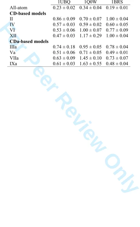
A plot of the time evolution of the root mean square deviation (RMSD)
calculated over all atoms of the systems versus the initially optimized protein structures is displayed in SI 7. Mean values and their standard deviation are reported in Table 3. Regardless of the protein system, all mean RMSD values are larger than corresponding all-atom values when a RPCM is applied. Among the RPCMs, IV and Va appear to be characterised by the lowest RMSD values, with however a slight discrepancy to this rule for model XII applied to Ubiquitin with RMSD = 0.47 nm, and for model IXa applied to Barnase–Barstar with RMSD = 0. 48 nm. The highest values, 1.17, 1.45, and 1.63 nm, are observed for structure 1Q0W modelled with XII, VIIa and IXa,
respectively. They are due to a progressive decomplexation of the two protein partners as illustrated using snapshots of the last MD frame (Figure 2) and lead to higher
standard deviations of 0.29, 0.10, and 0.55 nm, respectively (Table 3). In the case of 1BRS, the structure modelled using II and XII differs the most from the starting protein conformation, with a mean RMSD = 1.00 nm. The simulated structure is however relatively stable, with a standard deviation of 0.04 nm in each case. There actually is a slight interpenetration of Barnase into the structure of Barstar, due to the strong
deconstruction of the complex structure with model II, while, with model XII, one observes a strong unfolding of the Barstar amino acid sequence 190 to 199 interacting along the Barnase segment 37 to 30 (SI 8).
3.2 Structure analysis
The analysis of maps reporting the mean shortest residue-residue distances (SI9), shows that the least deconstructing model is Va, i.e., the model constructed with charges fitted on all-atom Coulomb forces calculated at grid points ranging between 1.2 and 2.0 times 3 4 5 6 7 8 9 10 11 12 13 14 15 16 17 18 19 20 21 22 23 24 25 26 27 28 29 30 31 32 33 34 35 36 37 38 39 40 41 42 43 44 45 46 47 48 49 50 51 52 53 54 55 56 57 58 59 60
For Peer Review Only
the van der Waals radius of the atoms, with a separate treatment of main chain and side chain charges. In structure 1UBQ modelled using II and IIIa, some of the close
contacts, especially those occurring between amino acid residues 30 to 40 and 69 to 75 or between residues 15 to 25 and 40 to 50, i.e., β-strands, are missing. Models IV and Va allow to retain the main features of the 3D folds, as also observed for the two other protein systems, while II, IXa, and XII show a deconstruction of Ubiquitin in 1Q0W as well as a displacement of Vps27 UIM-1 away from Ubiquitin. In the case of 1BRS, IIIa and IXa also provide distance maps that are similar to the all-atom results, with slight discrepancies for Barnase and Barstar, respectively. With IIIa, amino acid sequences 20 to 38 and 38 to 50 have a reduced number of close contacts due to the unfolding of the sequence 20 to 50 into a loose loop, while with IXa, sequences 111 to 131 and 170 to 199 have a reduced number of close contacts due to a deconstruction of the involved helices and strands (SI 8). Nevertheless, secondary structures (SI 10) as well as final snapshots of the MD trajectories (Figure 2) show at least a partial conservation of the molecular structure. In the case of structure 1UBQ, IV, Va, VI, and XII seem to favour the helix moeity versus the other representations while all selected models but II, IIIa, Va, and VIIa, let appear rather well preserved β-strands (SI 10). Additionally, the mean gyration radius of structure 1UBQ, calculated from the IV- and Va-based MD
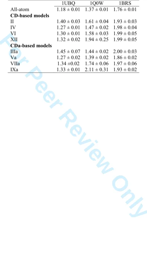
trajectories, 1.27 nm in both cases, is closer to the all-atom value, 1.18 nm (Table 4). They are also associated with relatively low standard deviation values. Snapshots taken at the final MD step (Figure 2) show that IV, Va, IXa, and XII preserve some of the regular secondary structure elements of Ubiquitin, i.e., α and β structural elements. The corresponding RMSD value calculated versus the initially optimized structure using VMD [48] adopt the lowest RMSD values, i.e., below or close to 0.5 nm (Table 5). For example, IV and Va present values of 0.484 and 0.421 nm, respectively. Model XII 3 4 5 6 7 8 9 10 11 12 13 14 15 16 17 18 19 20 21 22 23 24 25 26 27 28 29 30 31 32 33 34 35 36 37 38 39 40 41 42 43 44 45 46 47 48 49 50 51 52 53 54 55 56 57 58 59 60
For Peer Review Only
seems to even better preserve the global shape of the protein with a RMSD value of 0.355 nm.
In the case of structure 1Q0W, II and VI appear to completely miss the helix structures (SI 10), while XII misses the β-strands. Models IIIa and IV have a stronger trend to preserve these two kinds of secondary structure elements, while Va and VIIa still show a progressive loss of the secondary structure. Model IXa appears to preserve part of the secondary structure of Ubiquitin, as also seen from Figure 2, while the helix structure of the ligand is, in all RPCMs, strongly deconstructed. As for uncomplexed Ubiquitin, the RMSD value of the final protein conformation calculated versus the initially optimized structure stay close to 0.5 nm when using IV and Va (Table 5).
Regarding the Barnase–Barstar complex, models Va and IXa allow to maintain a number of α-helical structures, especially the very first helix of Barnase, as well as a higher number of β-strands than the other RPCMs (Figure 2 and SI 10). Structures simulated by these two models are very stable, especially when using Va. Additionally, for these two RPCMs, regions of the distance maps involving the first 40 Barnase residues let appear close contacts, similarly to the all-atom case (SI 9). Again, such more satisfying models come with the lowest mean RMSD values, below 0.5 nm (Table 3) and with gyration radii rG that are the closest to the corresponding all-atom values
(Table 4). The closest agreement between rG values is provided by Va, with a value of
1.86 versus 1.76 nm for the all-atom model. It also appears to be the less varying value during the 20 ns MD trajectory, with the lowest standard deviation value, 0.02 nm (Table 4). Finally, the RMSD value that is associated with the final frame is close to 0.5 nm, as already observed for the best models of the two other protein systems (Table 5). 3 4 5 6 7 8 9 10 11 12 13 14 15 16 17 18 19 20 21 22 23 24 25 26 27 28 29 30 31 32 33 34 35 36 37 38 39 40 41 42 43 44 45 46 47 48 49 50 51 52 53 54 55 56 57 58 59 60
For Peer Review Only
3.3 Backbone dynamics
An analysis of the Cα root mean square fluctuations (RMSF) shows that the motions of the amino acid residues can be strongly enhanced when one selects a RPCM (Figure 3). Large deviations, calculated as the RMSD between the RPCM and all-atom RMSFs, are even observed for models like IXa and XII when applied to structure 1Q0W (Table 6). In that case, RMSD values of 0.873 and 0.651 nm are obtained, respectively.
Nevertheless, the RMSD values reported in Table 6 are among the lowest ones for IV and Va, with values of 0.055 and 0.111 nm for structures 1UBQ and 1Q0W, and 0.116, 0.158, and 0.095 nm, for 1UBQ, 1Q0W, and 1BRS, respectively. Correlation
coefficients κ between the all-atom and RPCM-based RMSF values are calculated using:
( ) ( ) 1 RPCM atom all RPCM atom all N residues No.of 1 RPCM atom -all
u u u u N i i (4) where u stands for the RMSF values. ū and ζ are the average and the standard deviation of the u values for a given protein structure, respectively. As reported in Table 6, correlation coefficient values can be well below 1, especially for the two complex systems 1Q0W and 1BRS. This illustrates that the fluctuation pattern of the values u calculated for the all-atom trajectory is not systematically well reproduced by theRPCMs. However, κ has the highest values when obtained from II-, IV-, and IXa-based MD simulations, for 1UBQ, 1Q0W, and 1BRS, respectively. On the whole, IV and Va that are built using the same fitting conditions (Table 1) provide correlation coefficients that rank among the highest values for each protein system, with values of 0.910, 0.840, 0.590, and 0.835, 0.708, and 0.577, respectively. Contrarily, II and IIIa that are,
generally, characterised by high RMSD and low κ values, are more likely to favour κ (kappa) ζ (sigma) ū (u bar) 3 4 5 6 7 8 9 10 11 12 13 14 15 16 17 18 19 20 21 22 23 24 25 26 27 28 29 30 31 32 33 34 35 36 37 38 39 40 41 42 43 44 45 46 47 48 49 50 51 52 53 54 55 56 57 58 59 60
For Peer Review Only
complex system.
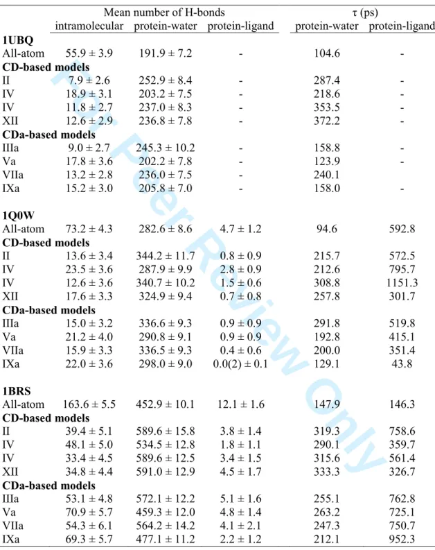
3.4 Hydrogen bond networks
The default parameters of hydrogen bonds in the GROMACS analysis tools are, for the H-acceptor distance and the donor-H-acceptor angle, set to 0.35 nm and 30°,
respectively. The analysis of intra- and intermolecular H-bonds occurring in all protein structures provided results that are given in Table 7. The Table shows that, consistently with values obtained previously,[20,22] the number of intramolecular H-bonds is drastically reduced when using RPCMs. For structure 1UBQ, one observes a reduction factor of 7 between the number of H-bonds in the all-atom model, i.e., 55.9, and in model II, i.e., 7.9. For all three structures, IV, Va, and IXa, are the least disagreeing models versus the all-atom ones. The decrease in the number of H-bonds mainly originates from the absence of any charge on the N and H atoms of the main chain, and on selected atoms of side chains, e.g., arg and lys. In addition, the absence of any clear maximum in the intramolecular H-bond angle distribution functions originates from a loss in the orientational character of the intra- H-bonds (Figure 4 and SI 11). The features presented in Figure 4 for 1UBQ only are also valid for the other protein structures and RPCMs, as illustrated in SI 11. Contrarily, RPCMs lead to an apparent increase in the number of protein-water H-bonds. This is related to the less structured water network as shown by radial distribution functions which illustrate a less well defined first solvation shell (Figure 5 and SI 12). The features presented in Figure 5 for 1UBQ are generalised to the other two protein structures and RPCMs, as illustrated in SI 12. However, the number of such H-bonds, 191.9 in the all-atom case of structure 1UBQ, is almost preserved when one considers the standard deviations of the numbers obtained with IV, Va, and IXa. Reduced point charge distributions Va and IXa are also appropriate to model 1Q0W and 1BRS.
3 4 5 6 7 8 9 10 11 12 13 14 15 16 17 18 19 20 21 22 23 24 25 26 27 28 29 30 31 32 33 34 35 36 37 38 39 40 41 42 43 44 45 46 47 48 49 50 51 52 53 54 55 56 57 58 59 60
For Peer Review Only
The distribution of water molecules in the vicinity of the protein surface is illustrated using radial distribution functions (Figure 5 and SI 12). As expected for the all-atom models, g(surf-Ow) indeed lets appear two peaks, the first one being located at
about 0.2 nm which originates from the closest water molecules interacting through H-bonds with the protein surface atoms, and a second peak, at about 0.26 nm [36,38]. Those two peaks define the first solvation shell of the proteins. In the RPCM results, the first peak of g(surf-Ow) clearly vanishes but is still present in the g(surf-Hw)
distributions (Figure 5). The layer of the closest Ow atoms appears to be displaced
towards larger distances and is overlapped by the second peak of Ow atoms. A high
amount of water molecules are thus oriented differently when a RPCM is used. The dynamics of protein-water H-bonds can be characterised through the so-called H-bond autocorrelation functions:
h t h h t C( ) (0) ( ) (5) where h(t) is assigned a value of 1 or 0 if a particular pair of atoms is H-bonded or not. The approach that was applied to evaluate overall correlation times η associated with
C(t), is:
0 ) ( dtt C (6) Values of η are reported in Table 7. They show that protein-water H-bonds are best approximated by Va and IXa for the three protein systems. For examples, mean values of 459.3 and 477.1 are provided by those two models, respectively, and compare rather well to the all-atom value of 452.9. As reported before [20], η is largelyincreased when using a RPCM, regardless of the protein structure. It illustrates a slower η (tau) 3 4 5 6 7 8 9 10 11 12 13 14 15 16 17 18 19 20 21 22 23 24 25 26 27 28 29 30 31 32 33 34 35 36 37 38 39 40 41 42 43 44 45 46 47 48 49 50 51 52 53 54 55 56 57 58 59 60
For Peer Review Only
surface or to the greater short-range electrostatic interactions occurring due to large partial charges [20]. Besides the fact that the mean numbers of protein-ligand H-bonds are reduced versus the all-atom case (Table 7), their associated values of η have no definite trends in common to the two complexes. They however tend to show an increased lifetime for such H-bonds in the case of structure 1BRS, all η being larger than the all-atom value of 146.3 ps. A deeper analysis of the effect of the RPCM on the interface solvent molecules can be seen as a perspective to the present work by avoiding any changes in the protein conformations from one simulation to another. This can be achieved by simulating rigid protein structures.
3.5 Energetics
For each MD frame generated using a RPCM, the corresponding all-atom values of various energy terms were obtained through post-processing calculations. Linear
regression calculations were then achieved for the RPCM versus all-atom energy terms: I
E S
ERPCM allatom (7)
where S and I stand for the slope and the intercept of the linear equations, respectively. The determination coefficient R, S and I are reported in SI 13 to SI 15, respectively. Examination of the data shows that the Cb_14 terms, i.e., the Coulomb interaction potentials between atoms separated by three chemical bonds, are the most affected contributions. Indeed, the R and S values that are associated with those contributions are largely below 1. This implies that if one study, for instance, rigid systems by freezing dihedrals, the RPCMs should be well suited for electrostatic calculations, as already shown in our work about potassium ion channels [18,49]. Coulomb short-range (Cb_SR) regression data behave a lot better, with R and S close to 1. One even notices that while the intramolecular protein-protein Cb_SR (p-p) slope is almost always lower 3 4 5 6 7 8 9 10 11 12 13 14 15 16 17 18 19 20 21 22 23 24 25 26 27 28 29 30 31 32 33 34 35 36 37 38 39 40 41 42 43 44 45 46 47 48 49 50 51 52 53 54 55 56 57 58 59 60
For Peer Review Only
than 1, the intermolecular protein-non protein Cb_SR (p-np) slope can be larger than 1, which means that these energy terms can be slightly over-estimated, especially when using models with charges located away from the atom locations, i.e., II, IV, VI, and XII. On the whole, R and S associated with the total energy Etot are almost always of the order of 0.99. Exceptions occur for 1Q0W modelled with VI and XII for which R and S can be slightly lower, about 0.98. It is uneasy to classify the models as more or less satisfying based on the R and S values. One can however notices that the best models so far, Va and IXa, all have a Cb_SR (p-np) slope that is lower than 1, contrarily to all other models. To inspect the deviation of the energy values from their all-atom counterpart, intercept values of the linear regressions were also analysed (SI 15). Models Va and IXa almost systematically present the lowest absolute intercept values. It is actually always the case for Cb-14, Cb-SR, Epot, and Etot. This may be related to the fact that both Va and IXa have similar distributions of main chain charge values (Table 1). In conclusion, a better approximation of the Cb_14 term occurs when charges are set on the atoms of the proteins and are fitted from Coulomb forces rather than from potentials.
More generally, sets of force-fitted charges like IV and Va allow to
systematically better approximate all-atom forces than II and IIIa at very short distances from the protein atoms, i.e., between 1.0 and 1.4 times the van der Waals radius of the atoms. Indeed, the error function y defined in equation (3) presents an averaged
decrease of 14 and 18 % for model IV versus II and Va versus IIIa, respectively. In the range of distances between 1.4 and 10.0 times the van der Waals radius of the atoms, potential- and force-based charges behave similarly when evaluating forces, with a slight averaged increase of 6 and 4 % for IV versus II and Va versus IIIa, respectively.
Finally, increasing the distance range of force values away from the protein 3 4 5 6 7 8 9 10 11 12 13 14 15 16 17 18 19 20 21 22 23 24 25 26 27 28 29 30 31 32 33 34 35 36 37 38 39 40 41 42 43 44 45 46 47 48 49 50 51 52 53 54 55 56 57 58 59 60
For Peer Review Only
atoms should apparently be combined with a single consideration of all charges in the fitting procedure, as in the case of IXa.
Model Va always performs the best for intra- and intermolecular Coulomb short-range terms, i.e., Cb_SR (p-p) and Cb_SR (p-np), respectively. For example, the Cb_14 intercept of Va for structure 1UBQ is 5587.5 kJ.mol-1 versus 9169.0 for model IIIa. Model IV is also among the best model to consider when using charges that are located away from the molecular skeleton. Again, for structure 1UBQ, the intercept value is 9467.7 versus 12097.1 for model II. On the whole, intercept values are lower for the CDa-based models than they are for the CD-based ones. Among the CD-based models, IV performs the best for all energy terms and all protein systems except for the
reciprocal term Cb_recip. Models II and XII, as well as IIIa and VIIa are, on the whole, the less favourable models to consider in the CD-based and CDa-based family, respectively. This confirms the high potency of II and IIIa to rapidly provide various protein conformations, as studied in reference [22] for the Vps27 UIM-1–Ubiquitin complex system.
3.6 Protein-ligand contacts
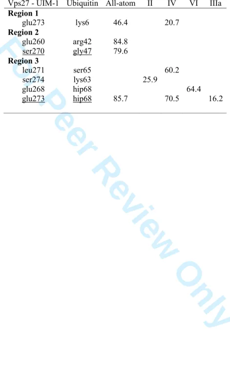
A detailed study of the contacts between protein partners in Vps27 UIM-1–Ubiquitin and Barnase–Barstar complexes is illustrated by Figure 6 and SI 16 that present the mean shortest distance between the amino acid residues of both partners averaged over the 20 ns MD trajectories. In the first case, one clearly distinguishes three regions extended along the Vps27 UIM-1 chain. The first region corresponds to the contacts occurring between the segment of amino acids 4 to 17 (259 to 272) of Vps27 UIM-1 and the β-strand 4 to 10 of Ubiquitin, while the second and third regions are due to contacts with β-strands 40 to 45 and 48 to 49, and β-strand 66 to 72, respectively. A pattern similar to the 1Q0W all-atom one was obtained when using IV. Model Va also 3 4 5 6 7 8 9 10 11 12 13 14 15 16 17 18 19 20 21 22 23 24 25 26 27 28 29 30 31 32 33 34 35 36 37 38 39 40 41 42 43 44 45 46 47 48 49 50 51 52 53 54 55 56 57 58 59 60
For Peer Review Only
presents the three regions but the first region appears to be more extended in the sense that almost all residues are in close contact with Ubiquitin, except for the central amino acids. This is due to the bending of Vps27 UIM-1 through its central residues (Figure 2). Highest occurrence frequency values of the protein-protein H-bonds, calculated using VMD [48] with cut-off distance and angle of 0.35 nm and 30°, are given in Table 8. Models for which no values were obtained are not reported. The Table shows, as already reported in Table 7, that H-bonds are less frequent and less numerous for the RCPMs than they are in the all-atom case. Model IV is however characterised by three Vps27 UIM-1– Ubiquitin H-bonds, i.e., glu273-lys6, leu271-ser65, glu273-hip68, occurring in regions 1 and 3. Models VI and VIIa present the three regions too, with reduced area (SI 16) due, respectively, to a drastic bending or extension of the ligand (Figure 2), while IXa and XII are strongly limited in their number of contacts due to the decomplexation of the ligand. In model XII, Vps27 UIM-1 still interacts with Ubiquitin through its C-terminal residue.
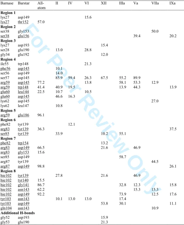
Model Va also allows to reproduce the main features of the Barnase–Barstar contact map pattern (Figure 6, SI 16). These features form a set of eight regions and are determined from the observed shortest distances (Figure 6). Among the eight areas reported in Table 9, region #3 is not listed in the Contact Map Database ABC2 [50]. It actually involves looser contacts observed along the MD trajectory. Contrarily, contacts detected in ABC2 and also appearing in the all-atom MD simulation have disappeared from the RPCM simulations. Those are lys27-thr152 (region #1), arg59-glu186 (region #5), arg83-tyr139 (region #7), and hie102-tyr140 (region #8). When one focusses on the protein-ligand H-bonds occurring with a frequency larger than 10 %, one notices that one or more H-bonds identified by ABC2 are detected using the all-atom MD simulation (Table 9), e.g., for region #1, the lys27-thr152 H-bond occurs with a 3 4 5 6 7 8 9 10 11 12 13 14 15 16 17 18 19 20 21 22 23 24 25 26 27 28 29 30 31 32 33 34 35 36 37 38 39 40 41 42 43 44 45 46 47 48 49 50 51 52 53 54 55 56 57 58 59 60
For Peer Review Only
frequency of 57.0 %. Models IXa, and XII let appear H-bonds in five different regions, but Va presents relatively high frequency values in the four areas it covers. For
examples, regions #2, #4, #7, and #8 are characterised by H-bond occurrence frequency values of 39.4, 89.9, 46.9, and 46.9 %, respectively. H-bonds between gly52 and asp193 as well as between gly53 and glu190 are also found with XII. They appear along the extended amino acid sequence 190-199 of Barstar as illustrated earlier (SI 8).
4. Conclusions and perspectives
Two reduced point charge distributions were considered for Molecular Dynamics (MD) simulations of three protein systems, i.e., Ubiquitin, Vps27 UILM-1–Ubiquitin, and Barnase–Barstar. The first distribution, based on charges located at critical points of smoothed amino acid charge density distribution functions calculated from Amber99 atomic charge values, involves two point charges on the main chain of each amino acid, precisely located on atoms C and O, and up to six charges for the side chain, mostly located away from atomic positions. In the second distribution, most of the charges are set at selected atom positions. Several sets of charge values were obtained by using different charge fitting conditions, i.e., based on electrostatic potential or forces, considering reference grid points located within various distance ranges from the protein atoms, with or without separate treatment of main chain and side chain charges.
The MD simulations were carried out using the program GROMACS with the Amber99SB force field, in TIP4P-Ew water, at 300 K. Energetic, structural, and dynamical information were retrieved from the analysis of the MD trajectories of the reduced point charge models (RPCMs) and discussed versus the all-atom model and available literature data. An emphasis was put on the global fold, the secondary structure elements of the proteins, their energetics and fluctuations, and the characterisation of H-bonds within the protein and with the solvent.
3 4 5 6 7 8 9 10 11 12 13 14 15 16 17 18 19 20 21 22 23 24 25 26 27 28 29 30 31 32 33 34 35 36 37 38 39 40 41 42 43 44 45 46 47 48 49 50 51 52 53 54 55 56 57 58 59 60
For Peer Review Only
On a structural point of view, one observed a progressive loss in the secondary structure of the proteins when RPCMs are used. They also lead to an increase of the gyration radius. Among the eight charge sets used in the paper, a model based on the use of Coulomb forces as reference values for charge fitting, i.e., model Va, better preserves some secondary elements, due to a better description of the short range 1-4 Coulomb energy terms, and limit the increase of the gyration radius. Precisely, charges of Va were fitted on all-atom Coulomb forces calculated at grid points ranging between 1.2 and 2.0 times the van der Waals radius of the atoms, with a separate treatment of main chain and side chain charges. Model Va is also seen as one of the best to approximate energy values and is among the models that limit the increase of the backbone dynamics observed with RPCMs. Model IXa, built by fitting all point charge values on Coulomb forces calculated at grid points ranging between 2.0 and 5.0 times the van der Waals radius of the atoms, also appears to be a reliable model. However, it leads to strong structural changes of the Vps UIM-1 helix. Fitting charges on a limited number of points is more efficient when electrostatic forces are taken as reference values most likely because it systematically improves the approximation of all-atom forces at short separations, thus leading to MD trajectories that better approximate the all-atom ones. Additionnally, it appears that Coulomb energy values are also closer to the all-atom ones.
The RPCMs do not favour the formation of a first hydration shell as clearly as the all-atom model does. They however allow the formation of solute-solvent H-bonds with geometrical properties similar to the all-atom case. Intra-protein H-bonds are differently described with no well-defined angle distributions. The mean number of intra-protein H-bonds is largely reduced versus the corresponding all-atom values, due 3 4 5 6 7 8 9 10 11 12 13 14 15 16 17 18 19 20 21 22 23 24 25 26 27 28 29 30 31 32 33 34 35 36 37 38 39 40 41 42 43 44 45 46 47 48 49 50 51 52 53 54 55 56 57 58 59 60
For Peer Review Only
to the decrease in the number of point charges, while the opposite trend is observed for the solute-solvent H-bonds, due to less-structured first solvation shells.
Following the work presented above, we will further focus on the RPCMs that allow major conformational changes in the protein structure, i.e., II and IIIa. Indeed, a work achieved on structure 1Q0W [22] showed that these charge models allow to generate particular conformations that appear to be stable ones through all-atom MD simulations.
It is also planned, as a longer term perspective, to combine a RPCM with a coarse-grained description of the protein structures.
Acknowledgments
The author thanks the referees for their useful comments regarding the manuscript, and Daniel Vercauteren, Director of the ‘Laboratoire de Physico-Chimie Informatique’ at the University of Namur, for fruitful discussions. Frédéric Wautelet and Laurent Demelenne are gratefully acknowledged for program installation and maintenance. This research used resources of the ‘Plateforme Technologique de Calcul Intensif (PTCI)’ (http://www.ptci.unamur.be) located at the University of Namur, Belgium, which is supported by the F.R.S.-FNRS. The PTCI is member of the ‘Consortium des Équipements de Calcul Intensif (CÉCI)’ ( http://www.ceci-hpc.be).
References
[1] Lindorff-Larsen K, Maragakis P, Piana S, Eastwood MP, Dror RO, Shaw DE. Systematic validation of protein force fields against experimental data. PLoS ONE. 2012;7:e32131/1-e321131/6.
[2] Beauchamp KA, Lin Y-S, Das R, Pande VS. Are protein force fields getting better? A systematic benchmark on 524 diverse NMR measurements. J. Chem. Theory Comput. 2012;8:1409-1414.
[3] Voth GA, editor. Coarse-graining of condensed phase and biomolecular systems. Boca Raton (FL): CRC Press; 2009.
[4] Hills RD Jr, Lu L, Voth GA. Multiscale coarse-graining of the protein energy landscape. PLoS Comput. Biol. 2010;6:e1000827/1-e1000827/12.
3 4 5 6 7 8 9 10 11 12 13 14 15 16 17 18 19 20 21 22 23 24 25 26 27 28 29 30 31 32 33 34 35 36 37 38 39 40 41 42 43 44 45 46 47 48 49 50 51 52 53 54 55 56 57 58 59 60
For Peer Review Only
[5] Imai K, Mitaku S. Common pattern of coarse-grained charge distribution of structurally analogous proteins. Chem-Bio. Inform. J. 2003;3:194-200.
[6] Skepö M, Linse P, Arnebrant T. Coarse-grained modeling of proline rich protein 1 (PRP-1) in bulk solution and adsorbed to a negatively charged surface. J. Phys. Chem. B. 2006;110:12141-12148.
[7] Pizzitutti F, Marchi M, Borgis D. Coarse-graining the accessible surface and the electrostatics of proteins for protein-protein interactions. J. Chem. Theory Comput. 2007;3:1867-1876.
[8] Monticelli L, Kandasamy SK, Periole X, Larson RG, Tieleman DP, Marrink SJ. The MARTINI coarse-grained forcefield: Extension to proteins. J. Chem. Theory Comput. 2008;4:819-834.
[9] DeVane R, Shinoda W, Moore PB, Klein ML. Transferable coarse grain nonbonded interaction model for amino acids. J. Chem. Theory Comput. 2009;5:2115-2124.
[10] Nielsen SO, Lopez CF, Srinivas G, Klein ML. Coarse grain models and the computer simulation of soft materials. J. Phys.: Condens. Matter. 2004;16:R481-R512.
[11] Leherte, Guillot B, Vercauteren DP, Pichon-Pesme V, Jelsch C, Lagoutte A, Lecomte C. Topological analysis of proteins as derived from medium and high resolution electron density: Applications to electrostatic properties. In: Matta CF, Boyd RJ, editors. The Quantum Theory of Atoms in Molecules - From Solid State to DNA and Drug Design. Weinheim (D): Wiley-VCH; 2007, p. 285-316. [12] Shen H, Li Y, Ren P, Zhang D, Li G. Anisotropic coarse-grained models for
proteins based on Gay-Berne and electric multipole potentials. J. Chem. Theory Comput. 2009;5:2115-2124.
[13] Francl MM, Chirlian LE. The plus and minuses of mapping atomic charges to electrostatic potentials. Rev. Comput. Chem. 2000;14:1-31.
[14] Curcó D, Nussinov R, Alemán C. Coarse-grained representation of β-helical protein building blocks. J. Phys. Chem. B. 2007;111:10538-10549.
[15] Terakawa T, Takada S. RESPAC: Method to determine partial charges in coarse-grained protein model and its application to DNA-binding proteins. J. Chem. Theory Comput. 2014;10:711-721.
[16] Basdevant N, Borgis D, Ha-Duong T. A coarse-grained protein-protein potential 3 4 5 6 7 8 9 10 11 12 13 14 15 16 17 18 19 20 21 22 23 24 25 26 27 28 29 30 31 32 33 34 35 36 37 38 39 40 41 42 43 44 45 46 47 48 49 50 51 52 53 54 55 56 57 58 59 60
For Peer Review Only
[17] Berardi R, Muccioli L, Orlandi S, Ricci M, Zannoni C. Mimicking electrostatic interactions with a set of effective charges: A genetic algorithm. Chem. Phys. Lett. 2004;389373-389378.
[18] Leherte L, Vercauteren DP. Coarse point charge models for proteins from smoothed molecular electrostatic potentials. J. Chem. Theory Comput. 2009;5:3279-3298.
[19] Borodin O, Smith GD. Force Field Fitting Toolkit. The University of Utah. http://www.eng.utah.edu/~gdsmith/fff.html (Accessed 26 Aug. 2009). [20] Leherte L, Vercauteren DP. Comparaison of reduced point charge models of
proteins: Molecular dynamics simulations of Ubiquitin. Sci. China Chem. 2014;57:1340-1354.
[21] Wang Y, Noid WG, Liu P, Voth GA. Effective force coarse-graining. Phys. Chem. Chem. Phys. 2009;11:2002-2015.
[22] Leherte L, Vercauteren DP. Evaluation of reduced point charge models of proteins through molecular dynamics simulations: Application to the Vps27 UIM-1–Ubiquitin complex. J. Mol. Graphics Model. 2014;47:44-61.
[23] Wang J, Cieplak P, Kollman PA. How well does a restrained electrostatic potential (RESP) model perform in calculating conformational energies of organic and biological molecules, J. Comput. Chem. 2000;21:1999-2012. [24] Vijay-Kumar S, Bugg CE, Cook WJ. Structure of Ubiquitin refined at 1.8 Å
resolution. J. Mol. Biol. 1987;194:531-544.
[25] Swanson KA, Kang RS, Stamenova SD, Hicke L, Radhakrishnan I. Solution structure of Vps27 UIM–Ubiquitin complex important for endosomal sorting and receptor downregulation. EMBO J. 2003;22:4597-4606.
[26] Buckle AM, Schreiber G, Fersht AR. Protein-protein recognition: Crystal structural analysis of a Barnase–Barstar complex at 2.0 Å resolution. Biochemistry 1994;33:8878-8889.
[27] Dolinsky TJ, Nielsen JE, McCammon JA, Baker NA. PDB2PQR: An automated pipeline for the setup of Poisson-Boltzmann electrostatics calculations. Nucl. Acids Res. 2004;32:W665-W667.
[28] PDB2PQR, An automated pipeline for the setup, execution, and analysis of Poisson-Boltzmann electrostatics calculations. 2007. SourceForge Project Page. http://pdb2pqr.sourceforge.net/ (Accessed 31Aug. 2009)
3 4 5 6 7 8 9 10 11 12 13 14 15 16 17 18 19 20 21 22 23 24 25 26 27 28 29 30 31 32 33 34 35 36 37 38 39 40 41 42 43 44 45 46 47 48 49 50 51 52 53 54 55 56 57 58 59 60
For Peer Review Only
[29] Singh UC, Kollman PA. An approach to computing electrostatic charges for molecules. J. Comput. Chem. 1984;5:129-145.
[30] Hess B, Kutzner C, van der Spoel D, Lindahl E. GROMACS 4: Algorithms for highly efficient, load-balanced, and scalable molecular simulation. J. Chem. Theory Comput. 2008;4:435-447.
[31] Pronk S, Páll S, Schulz R, Larsson P, Bjelkmar P, Apostolov R, Shirts MR, Smith JC, Kasson PM, van der Spoel D, Hess B, Lindahl E. GROMACS 4.5: A high-throughput and highly parallel open source molecular simulation toolkit. Bioinformatics 2013;29:845-854.
[32] Showalter SA, Brüschweiler R. Validation of molecular dynamics simulations of biomolecules using NMR spin relaxation as benchmarks: Application to the AMBER99SB force field. J. Chem. Theory Comput. 2007;3:961-975.
[33] Bernstein FC, Koetzle TF, Williams GJ, Meyer Jr EE, Brice MD, Rodgers JR, Kennard O, Shimanouchi T, Tasumi M. The Protein Data Bank: A computer-based archival file for macromolecular structures. J. Mol. Biol. 1977;112:535-542.
[34] Horn HW, Swope WC, Pitera JW, Madura JD, Dick TJ, Hura GL, Head-Gordon T. Development of an improved four-site water model for biomolecular
simulations: TIP4P-Ew. J. Chem. Phys. 2004;120:9665-9678.
[35] Abscher R, Schreiber H, Steinhausser O. The influence of a protein on water dynamics in its vicinity investigated by molecular dynamics simulation. Proteins 1996;25:366-378.
[36] Dastidar SG, Mukhopadhyay C. Structure, dynamics, and energetics of water at the surface of a small globular protein: A molecular dynamics simulation. Phys. Rev. 2003;68:021921.
[37] Schröder C, Rudas T, Boresch S, Steinhauser O. Simulation studies of the protein-water interface. I. Properties at the molecular resolution. J. Chem. Phys. 2006;124:234907/1–234907/18.
[38] Virtanen JJ, Makowski L, Sosnick TR, Freed KF. Modeling the hydration layer around proteins: HyPred. Biophys. J. 2010;99:1611-1619.
[39] Ganoth A, Tsfadia Y, Wiener R. Ubiquitin: Molecular modeling and simulations. J. Mol. Graphics Mod. 2013;46:29-40.
[40] Hurley JH, Lee S, Prag G. Ubiquitin-binding domains. Biochem. J. 3 4 5 6 7 8 9 10 11 12 13 14 15 16 17 18 19 20 21 22 23 24 25 26 27 28 29 30 31 32 33 34 35 36 37 38 39 40 41 42 43 44 45 46 47 48 49 50 51 52 53 54 55 56 57 58 59 60
For Peer Review Only
[41] Lee L-P, Tidor B. Barstar is electrostatically optimized for tight binding to Barnase. Nature Struct. Biol. 2001;8:73-76.
[42] Dong F, Vijayakumar M, Zhou H-X. Comparison of calculation and experiment implicates significant electrostatic contributions to the binding stability of Barnase and Barstar. Biophys. J. 2003;85:49-60.
[43] Wang T, Tomic S, Gabdoulline RR, Wade RC. How optimal are the binding energetics of Barnase and Barstar? Biophys. J. 2004;87:1618-1630.
[44] Ababou A, van der Vaart A, Gogonra V, Merz Jr KM. Interaction energy decomposition in protein-protein association: A quantum mechanical study of Barnase–Barstar study. Biophys. Chem. 2007;125:221-236.
[45] Hoefling M, Gottschalk KE. Barnase–Barstar: From first encounter to final complex. J. Struct. Biol. 2010;171:52-63.
[46] Ulucan O, Jaitly T, Helms V. Energetics of hydrophilic protein-protein
association and the role of water. J. Chem. Theory Comput. 2014;10:3512-3524. [47] Urakubo Y, Ikura T, Ito N. Crystal structure analysis of protein-protein
interactions drastically destabilized by a single mutation. Prot. Sci. 2008;17:1055-1065.
[48] Humphrey W, Dalk A, Schulten K. VMD - Visual Molecular Dynamics. J. Mol. Graphics 1996;14:33-38.
[49] Leherte L, Vercauteren DP. Charge density distributions derived from smoothed electrostatic potential functions: Design of protein reduced point ch arge models. J. Comput. Aided Mol. Des. 2011;25:913-930.
[50] Peter W, Sam A, Volkhard H. ABC (Analyzing Biomolecular Contacts)-database. J. Integr. Bioinf. 2007;4:50-58.
3 4 5 6 7 8 9 10 11 12 13 14 15 16 17 18 19 20 21 22 23 24 25 26 27 28 29 30 31 32 33 34 35 36 37 38 39 40 41 42 43 44 45 46 47 48 49 50 51 52 53 54 55 56 57 58 59 60
For Peer Review Only
Figure captions
Figure 1. Location of point charges (black spheres) of the amino acid residues on (Top) critical points of smoothed charge density distribution functions, and (Bottom) selected atoms.
Figure 2. Final snapshots of the protein structures obtained from the last frames of 20 ns AMBER99SB-TIP4P-Ew MD trajectories at 300 K. Secondary structure elements are color-coded as follows: Coil (white), α-helix (blue), π helix (purple), 310 helix (grey),
β-sheet (red), β-bridge (black), bend (green), turn (yellow). For an interpretation of the references to colour, the reader is referred to the web version of the article.
Figure 3. RMSF of the Cα atoms of structures 1UBQ, 1Q0W, and 1BRS, obtained from 20 ns AMBER99SB-TIP4P-Ew MD trajectories at 300 K. (Plain line) All-atom, (dashed line) model IV, (dotted line) model Va. Residues of the protein complexes are
numbered 1 to 24 (Vps27 UIM-1) and 25 to 100 (Ubiquitin) for 1Q0W, and 1 to 110 (Barnase) and 111 to 199 (Barstar) for 1BRS.
Figure 4. Distance and angle distributions of the Ubiquitin (1UBQ)-water H-bonds obtained from 20 ns AMBER99SB-TIP4P-Ew MD trajectories at 300 K. (Plain line) All-atom, (dotted line) model Va.
Figure 5. Radial distribution functions of the Ubiquitin (1UBQ) surface atoms versus the water atoms, g(P-Ow) and g(P-Hw), obtained from 20 ns AMBER99SB-TIP4P-Ew
MD trajectories at 300 K. (Plain line) All-atom, (dotted line) model Va. Figure 6. Mean shortest protein-ligand distance maps as calculated from 20 ns AMBER99SB-TIP4P-Ew MD trajectories at 300 K for model Va. Encircled areas correspond to regions described in Tables 8 and 9. Distances are given in nm in the colour scale. For an interpretation of the references to colour, the reader is referred to the web version of the article.
3 4 5 6 7 8 9 10 11 12 13 14 15 16 17 18 19 20 21 22 23 24 25 26 27 28 29 30 31 32 33 34 35 36 37 38 39 40 41 42 43 44 45 46 47 48 49 50 51 52 53 54 55 56 57 58 59 60
For Peer Review Only
Table 1. Charge fitting conditions applied to generate various sets of reduced point charge models (RPCM) based on the previously developed models mCD (model II) and mCDa (model IIIa) [22].
Charge fitting conditions
RPCMa Reference gridb Separate treatment of main and side chain charges Range of valid grid values (Å) Range of charge values (|e-|) Average and standard deviation of the absolute charge values of
the main chain (|e-|) Charges and virtual site parameters CD-based models II MEP yes 1.2 – 2.0 -0.85 – 1.35 0.77 ± 0.09 [22] IV MEF yes 1.2 – 2.0 -0.80 – 1.03 0.69 ± 0.08 SI 1 VI MEF yes 2.0 – 5.0 -0.84 – 1.53 0.77 ± 0.09 SI 2 XII MEP yes 2.0 – 5.0 -0.87 –
1.92
0.79 ± 0.10 SI 3
CDa-based models
IIIa MEP yes 1.2 – 2.0 -0.81 – 1.03
0.73 ± 0.09 [22] Va MEF yes 1.2 – 2.0 -0.76 –
1.03
0.64 ± 0.07 SI 4 VIIa MEF yes 2.0 – 5.0 -0.79 –
1.09 0.73 ± 0.09 SI 5 IXa MEF no 2.0 – 5.0 -0.84 – 1.03 0.62 ± 0.10 SI 6 a
CD and CDa stand for models where point charges are located at the critical points of the charge density (CD) and at atoms, respectively.
b
MEP and MEF stand for molecular electrostatic potential and molecular electrostatic force, respectively. 3 4 5 6 7 8 9 10 11 12 13 14 15 16 17 18 19 20 21 22 23 24 25 26 27 28 29 30 31 32 33 34 35 36 37 38 39 40 41 42 43 44 45 46 47 48 49 50 51 52 53 54 55 56 57 58 59 60
For Peer Review Only
Table 2. Description of the protein systems simulated by Amber99SB-TIP4P-Ew MD using various point charge models.
Point charge model
All-atom
II IV VI XII IIIa Va VIIa IXa
1UBQ
# H2O 10369 10366 10366 10366 10366 10368 10366 10368 10368
# Point charges 1231 283 283 283 283 283 283 283 283 # Non-atomic point charges 0 84 84 84 84 2 2 2 2 Simulation box (nm) 6.89 6.89 6.89 6.89 6.89 6.89 6.89 6.89 6.89 Dipole moment (D) of the
optimized protein structure
217.8 221.9 230.1 226.1 222.6 231.2 236.1 231.6 237.6
1Q0W
# H2O 10553 10542 10542 10542 10542 10551 10551 10551 10551
# Point charges 1623 382 382 382 382 382 382 382 382 # Non-atomic point charges 0 112 112 112 112 3 3 3 3 Simulation box (nm) 6.95 6.95 6.95 6.95 6.95 6.95 6.95 6.95 6.95 Dipole moment (D) of the
optimized protein structure
210.2 205.2 216.3 210.1 208.6 212.9 218.3 212.5 218.4
1BRS
# H2O 18738 18916 18916 18723 18912 18740 18740 18739 18740
# Point charges 3161 786 786 786 786 786 786 786 786 # Non-atomic point charges 0 272 272 272 272 12 12 12 12 Simulation box (nm) 8.43 8.45 8.45 8.43 8.45 8.43 8.43 8.43 8.43 Dipole moment (D) of the
optimized protein structure
215.5 219.7 228.6 222.5 220.9 224.0 231.2 224.1 222.3 3 4 5 6 7 8 9 10 11 12 13 14 15 16 17 18 19 20 21 22 23 24 25 26 27 28 29 30 31 32 33 34 35 36 37 38 39 40 41 42 43 44 45 46 47 48 49 50 51 52 53 54 55 56 57
For Peer Review Only
Table 3. Mean RMSD values (nm) calculated versus the initially optimized structures, and their standard deviation, obtained from the analysis of the last 20 ns of the solvated
Amber99SB-based MD trajectories at 300 K. All atoms are considered in the calculations.
1UBQ 1Q0W 1BRS All-atom 0.23 ± 0.02 0.34 ± 0.04 0.19 ± 0.01 CD-based models II 0.86 ± 0.09 0.70 ± 0.07 1.00 ± 0.04 IV 0.57 ± 0.03 0.59 ± 0.02 0.60 ± 0.05 VI 0.53 ± 0.06 1.00 ± 0.07 0.77 ± 0.09 XII 0.47 ± 0.03 1.17 ± 0.29 1.00 ± 0.04 CDa-based models IIIa 0.74 ± 0.18 0.95 ± 0.05 0.78 ± 0.04 Va 0.51 ± 0.06 0.71 ± 0.05 0.49 ± 0.01 VIIa 0.63 ± 0.09 1.45 ± 0.10 0.73 ± 0.07 IXa 0.61 ± 0.03 1.63 ± 0.55 0.48 ± 0.04 3 4 5 6 7 8 9 10 11 12 13 14 15 16 17 18 19 20 21 22 23 24 25 26 27 28 29 30 31 32 33 34 35 36 37 38 39 40 41 42 43 44 45 46 47 48 49 50 51 52 53 54 55 56 57 58 59
For Peer Review Only
Table 4. Mean gyration radii rG (nm), and their standard deviation obtained from the analysis of the last 20 ns of the Amber99SB-TIP4P-Ew MD trajectories at 300 K.
1UBQ 1Q0W 1BRS All-atom 1.18 ± 0.01 1.37 ± 0.01 1.76 ± 0.01 CD-based models II 1.40 ± 0.03 1.61 ± 0.04 1.93 ± 0.03 IV 1.27 ± 0.01 1.47 ± 0.02 1.98 ± 0.04 VI 1.30 ± 0.01 1.58 ± 0.03 1.99 ± 0.05 XII 1.32 ± 0.02 1.94 ± 0.25 1.99 ± 0.05 CDa-based models IIIa 1.45 ± 0.07 1.44 ± 0.02 2.00 ± 0.03 Va 1.27 ± 0.02 1.39 ± 0.02 1.86 ± 0.02 VIIa 1.34 ±0.02 1.74 ± 0.06 1.97 ± 0.06 IXa 1.33 ± 0.01 2.11 ± 0.31 1.93 ± 0.02 3 4 5 6 7 8 9 10 11 12 13 14 15 16 17 18 19 20 21 22 23 24 25 26 27 28 29 30 31 32 33 34 35 36 37 38 39 40 41 42 43 44 45 46 47 48 49 50 51 52 53 54 55 56 57
For Peer Review Only
Table 5. RMSD (nm) of the final protein structure calculated versus the initially optimized structures using VMD [48] from the last 20 ns of the Amber99SB-TIP4P-Ew MD trajectories at 300 K. Only backbone atoms are considered in the calculations.
1UBQ 1Q0W 1BRS All-atom 0.123 0.236 0.136 CD-based models II 0.891 0.844 0.895 IV 0.484 0.537 0.705 VI 0.530 0.949 0.940 XII 0.355 1.727 0.905 CDa-based models IIIa 0.864 0.904 0.636 Va 0.421 0.543 0.409 VIIa 0.596 1.238 0.573 IXa 0.525 2.132 0.526 3 4 5 6 7 8 9 10 11 12 13 14 15 16 17 18 19 20 21 22 23 24 25 26 27 28 29 30 31 32 33 34 35 36 37 38 39 40 41 42 43 44 45 46 47 48 49 50 51 52 53 54 55 56 57 58 59
For Peer Review Only
Table 6. RMSD (nm) and correlation coefficient κ calculated between the simulated Cα RMSF values (RPCM versus all-atom) obtained from the analysis of the last 20 ns of the Amber99SB-TIP4P-Ew MD trajectories at 300 K. RMSD κ 1UBQ 1Q0W 1BRS 1UBQ 1Q0W 1BRS CD-based models II 0.130 0.204 0.214 0.919 0.599 0.192 IV 0.055 0.111 0.251 0.910 0.840 0.590 VI 0.086 0.407 0.360 0.846 0.528 0.310 XII 0.104 0.651 0.457 0.868 0.589 0.505 CDa-based models IIIa 0.308 0.100 0.209 0.380 0.680 0.191 Va 0.116 0.158 0.095 0.835 0.708 0.577 VIIa 0.145 0.415 0.267 0.880 0.720 0.334 IXa 0.071 0.873 0.102 0.849 0.681 0.655 3 4 5 6 7 8 9 10 11 12 13 14 15 16 17 18 19 20 21 22 23 24 25 26 27 28 29 30 31 32 33 34 35 36 37 38 39 40 41 42 43 44 45 46 47 48 49 50 51 52 53 54 55 56 57

![Table 5. RMSD (nm) of the final protein structure calculated versus the initially optimized structures using VMD [48] from the last 20 ns of the Amber99SB-TIP4P-Ew MD trajectories at 300 K](https://thumb-eu.123doks.com/thumbv2/123doknet/14509500.720681/36.918.200.663.208.997/table-protein-structure-calculated-initially-optimized-structures-trajectories.webp)