Design optimization of a 2D blade by means of milling
tool path
Christian Vessaza, Christophe Tournierb,∗, C´ecile M¨unchc, Fran¸cois Avellana
aEPFL, ´Ecole polytechnique f´ed´erale de Lausanne, Laboratory for Hydraulic Machines,
avenue de Cour 33 bis, 1007 Lausanne, Switzerland
bLURPA, ENS Cachan, Universit´e Paris Sud 11, 61 avenue du Pr´esident Wilson, 94235
Cachan, France
cHES SO Valais, Haute ´ecole sp´ecialis´ee de Suisse occidentale, Institut Syst`emes
industriels, Route du Rawyl 47, 1950 Sion, Switzerland
Abstract
In a conventional design and manufacturing process, turbine blades are modeled based on reverse engineering or on parametric modeling with Computer Fluids Dynamics (CFD) optimization. Then, only raises the question of the manu-facturing of the blades. As the design does not take into account machining constraints and especially tool path computation issues in flank milling, the ac-tual performance of the machined blade could not be optimal. In this paper, a new approach is used for the design and manufacture of turbine blades in order to ensure that the simulated machined surface produces the expected hydraulic properties. This consists in the modeling of a continuous tool path based on numerical simulation rather than the blade surface itself. Consequently, this paper aims at defining the steps of the proposed design approach including geo-metrical modeling, mesh generation, CFD simulation and genetic optimization. The method is applied on an isolated blade profile in a uniform water flow and results are compared to the conventional design process.
Keywords: Design for manufacturing, Tool path, Flank milling, Genetic optimization, Blades
1. Introduction 1
The design and machining process of blade surfaces consists in three steps 2
including Computer-Aided Design (CAD) modeling with CFD optimization of 3
the blade, tool path computation in the Computer-Aided Manufacturing (CAM) 4
software and machining of the part on a machine tool. In this process, the CAD 5
model is the reference model used by any other applications and it usually relies 6
on parametric curves and surfaces with geometrical continuity properties. 7
From a geometrical point of view, blade modeling is mostly performed by the 8
interpolation of a succession of 2D profiles along the spanwise direction. These 9
2D profiles are computed whether by the interpolation of a set of sampling 10
points computed by CFD software or directly by the use of parametric curves. 11
The main objectives of the parametric model are to ensure continuity between 12
the curves defining the 2D contour and to reduce the number of geometrical 13
parameters. 14
However, from a digital mock-up point of view, the degree of polynomial 15
curves and continuity between curves in the parametric model does not matter. 16
Indeed, the geometry of the CAD model is approximated by all the CAX appli-17
cations based on this model: CFD and Finite Element Analysis (FEA), which 18
generate meshes, visualization using tessellation and even tool path computa-19
tion, which discretizes surfaces into curves and curves into points as developed 20
hereafter. 21
During the CAM stage, a set of tool postures (tool position and tool axis 22
orientation) is computed according to a machining strategy [1]. Depending on 23
the design surface, machining is performed in 3 or 5-axis and in flank or end 24
milling. Usual CAM system algorithms for tool path computation rely on the 25
linear format, which is common in the machine tool Numerical Controllers (NC). 26
The surface to be machined is discretized into a set of curves and each curves 27
is discretized into polylines generating geometrical deviations compared to the 28
design. Furthermore, tool paths contain tangency discontinuities which leads 29
to slowdowns during machining and marks on the part due to chip section vari-30
ations during machining. Post-processors may convert linear tool paths into 31
polynomial curves. The polynomial trajectory is thus called off-line polynomial 32
trajectory [2] in opposition to on-line polynomial trajectory that corresponds to 33
polynomial trajectory calculated in real-time by the NC unit [3]. In both meth-34
ods, the polyline is interpolated by polynomial curves such as Bspline curves 35
according to a geometrical tolerance specified by the user. Consequently, in 36
the classical design approach, hydraulic optimization of the blade geometry can 37
provide an optimal design Xd∗, which probably could not be machined without 38
geometrical deviations. 39
40
To quickly design blades taking into account their machinability, a new 41
paradigm consists of placing the machining tool path on the heart of the design 42
process [4]. A continuous polynomial tool path is computed so that the envelop 43
of the tool movement, not the CAD model, is optimum with respect to the 44
hydraulic performances. Then, the optimization validates the surface geometry 45
resulting from a kinematical simulation of the machining, computed with the 46
Nbuffer method, and CAD model is the 3D representation of the simulation. 47
Manufacturing should be faster, geometric quality and perceived quality are 48
improved due to the use of a native polynomial tool path and hydraulic per-49
formance should better meet expectations. Therefore, the tool path is modeled 50
as a native set of Bspline curves and considered as the reference model. CAD 51
model and CFD/FEA models are then built on these curves through machining 52
simulation (Table1). 53
Table 1: Geometry modeling for the different approaches
Method CAD FEA/CFD CAM Post-Pro CNC
Conventional Curves Mesh Points Points Points
On line Curves Mesh Points Points Curves
Off line Curves Mesh Points Curves Curves
In the proposed approach, the optimal tool path Xt∗ is necessarily machin-54
able, from a kinematical point of view, but the hydraulic performance will be 55
different from that obtained with the conventional approach Xd∗. Indeed, there 56
is an infinite geometrical solutions to define the blade surface and only one hy-57
draulic optimal solution. As soon as the parametric models to define the design 58
or the tool path are stated, the range of solutions is reduced as well as the 59
probability of finding the ideal solution. Moreover, as both approaches gener-60
ate different geometric models, they do not necessarily share the same solution 61
space. Thus, numerical investigations has to be performed to compare hydraulic 62
performances of both approaches. 63
The real challenge would consist to compare both approaches in the case 64
of 5-axis flank milling of 3D blades. Indeed, this process presents a high re-65
moval material rate a better surface roughness [5]. This process is now widely 66
investigated for the machining of slender complex parts like impellers or turbine 67
blades but it generates undercut and overcut as blades are non developable ruled 68
surfaces or free-form surfaces. Extensive works have been carried out to reduce 69
overcuts and undercuts with cylindrical cutters [6,7,8], conical cutters [9,10] and 70
barrel cutters [11,12]. Still, geometrical deviations are not removed and futher-71
more, the link between those deviations and the hydraulic performances of the 72
blades has not been investigated. 73
However, full 3D modeling for twisted blades made of non developable sur-74
faces requires a lot of tests and expensive computational time to setup the 75
process and the evidence of the success of the proposed approach is not guaran-76
teed. The purpose of this paper is thus to set-up and compare the classical and 77
proposed paradigm to design hydraulic profiles made with developable ruled 78
surfaces. Nevertheless, the use of polynomial curves such as Bezier curves to 79
model the designed profile and the tool path makes this test case relevant. In-80
deed, the ideal tool path for machining the profile is an offset curve of the profile 81
which equation is known as a rational function. As it is impossible to model the 82
offset curve of a polynomial curve by any polynomial curve, we therefore are 83
dealing with a case which is identical to the machining of non-developable ruled 84
surfaces where Xd∗ and Xt∗ solutions may be close but will never be identical. 85
The paper is organized as follows: in section 2, a parametric model is pro-86
posed based on a literature review of 2D profile parameterization. Then, the 87
optimization process is presented in section 3, which includes geometrical mod-88
eling for both approaches, the CFD simulation and the genetic optimization 89
loop. In section 4, numerical investigations are performed on a single blade in 90
order to compare both approaches. 91
2. 2D blades modeling 92
Two main approaches to design blades are found in the literature: the Shape 93
Inverse Design (SID) and the Global Shape Optimization (GSO) [13,14]. In 94
the SID methods, the designer usually starts from an initial blade geometry 95
and performance and inputs the desired modifications to the performance. SID 96
methods need few iterations to generate a new shape that duplicates the desired 97
surface flow parameters. However, this method requires an initial blade geom-98
etry computed using a direct approach. In opposition, GSO methods consist 99
in modifying the geometry of the blades until the flow performance is achieved. 100
Methods based on GSO have been developed more recently due to the required 101
computational effort to test and optimize a set of parameters. 102
2D profiles are computed either by the interpolation of a set of sampling 103
points computed by CFD software [15] or directly by the use of parametric 104
curves. Two main variants exist to define the parametric curves [16]. The 105
Camber-Curve + Thickness technic and the Direct Profiling technic. The camber-106
curve defines a skeleton and the thickness distribution defines the sides of the 107
profile [17]. This kind of modeling is not well appropriate to define a 2D profile 108
in parametric CAD systems if implicit formulation of the thickness law or of the 109
blade turning angle are used as in [18,19]. A typical example is the definition 110
of NACA 2D profiles, which are imported as sampling points in CAD systems 111
and then re-interpolated. 112
In the method proposed by Koini et al. [20] the camber line is described 113
by a NURBS curve of second degree with three control points (rational Bezier 114
curve). The suction and pressure sides are modeled as Bspline curves defined 115
by control points or interpolation points. The position of these points is defined 116
by a curvilinear abscissa and a normal distance to the camber line. 117
Different works have been published using the direct profile modeling [13,21,24]. 118
The main objective is to ensure continuity between the curves defining the 2D 119
contour and to reduce the number of geometrical parameters. Pritchard [21] 120
proposed a geometrical model based on polynomial curves in 1985. The 2D 121
profile consists in five concatenated curves connected in tangency (C1). The 122
advantage of this model is the reduced number of parameters (9). 123
The model proposed by Pierret et al. [22] consists in three Bezier curves and 124
a circle to design the trailing edge. The connection between the pressure and 125
the suction side at the leading edge ensures a continuous curvature. 126
Anders et al. [23] propose to model the 2D profile by using two Bezier curves 127
of degree 5 for the suction and pressure sides and circles or ellipses to describe 128
the leading and trailing edges. Tangency continuity is ensured at the junction 129
but not curvature continuity. This model leads to 20 parameters. 130
Other methods use only polynomial curves to define the 2D profile. The 131
method proposed by Buche et al. [24] consists in modeling the profile with 132
four polynomial Bezier curves of degree 5 connected in curvature. 16 of the 48 133
required parameters are set by imposing curvature continuity at the junctions. 134
The remaining 32 parameters are translated into engineering parameters and 135
some of them are set to default values leading finally to 19 variable parameters. 136
In [25], Giannakoglou used two Bezier curves of degree 5 to model the pres-137
sure side and the suction side as well as the leading (LE) and trailing (TE) 138
edges. Both curves shared the same starting and ending points at the LE and 139
TE and ensure tangency continuity at the LE. This parameterization yields to 140
14 parameters. 141
Goel [26] also used two Bezier curves to model the pressure side and the 142
suction side as well as the leading and trailing edges of thick airfoils for high 143
pressure turbines. 144
Table 2: Number of design parameters
Method Number of parameters
Pritchard 1985 9 Giannakoglou 2002 14 Goel 2009 14 Pierret et al 1999 15 Dennis et al 1999 17 Buche et al. 2003 19 Anders et al 2008 20 Korakianitis et al. 1993 35
Koini et al. 2009 Unspecified
The method proposed by Ghaly et al. [15] consists in approximating an 145
initial 2D profile by a single Nurbs curve and optimizing the design by moving 146
the Nurbs control points. The degree of the curve is not specified. 147
In [13], the profiles of suction and pressure surfaces are modeled as two 148
splines of degree 4. The leading edge is treated separately as a line + thickness 149
distribution. The construction ensures a third derivative continuity with the 150
suction and pressure splines. 151
Many combinations of curves are presented to model 2D profiles of turboma-152
chines. Among the criteria for discriminating methods, the order of continuity 153
at the connection between the curves and the number of design parameters is 154
considered (Table 2). Indeed, fewer parameters lead to shorter computation 155
time but reduce the variety of possible blade shapes. 156
In the framework of the optimization of hydraulic turbines or impellers, the 157
method proposed by Koini et al. [20] is adopted to design the blades with a 158
camber line and a thickness law to define the suction and pressure sides. The 159
first advantage is the use of a camber line, which shape is directly linked to 160
hydraulic parameters such as inlet and outlet angles (β1and β1). This method 161
also presents the advantage of an explicit parametric modeling, which is suited 162
to model the tool path as polynomial curves as well as the design in CAD 163
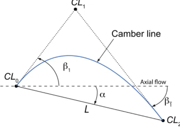
softwares. The camber line is defined as a Bezier curve CL(u) (Eq. 1) of degree 164
2 (m = 2) defined by three control points, that is to say 6 parameters. 165 CL(u) = m X i=0 Bim(u) · CLi with u ∈ [0, 1] (1)
The first control point CL0 is located on the leading edge and the last one 166
CL2 on the trailing edge (Fig. 1). The middle point CL1 is located at the 167
intersection between the lines defined with the inlet and outlet angles β1 and 168
β1. If a point of the camber line is considered as fixed, only 4 parameters are 169
required to define it (3 angles and 1 length). 170 CL 1 CL 0 CL 2
L
Axial ow 1 1 Camber lineFigure 1: Camber line modeling with Bezier curve
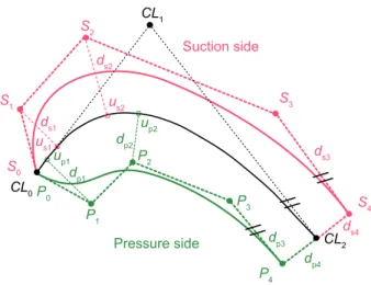
Suction and pressure sides are defined by two Bezier curves of degree 4, S(t) 171
and P (t), connected at the leading edge. Each control point Si or Pi of the 172
suction and pressure sides (except for i = 3) is defined by the abscissa u on the 173
camber line and the distance d (Fig. 2). 174
Si= CL(usi) + dsi· n (2)
175
Pi= CL(upi) + dpi· n (3)
The trailing edge, which is defined by the segment S4P4, is sharp to model 176
real hydraulic blades. The full model is entirely defined by a maximum of 24 177
S 0 S 1 S 2 S 3 S 4 u s1 u s2 d s1 d s2 d s3 d s4 P 2 P 1 P 0 P 3 P 4 Suction side Pressure side u p1 u p2 d p1 d p4 d p3 d p2 CL 1 CL 0 CL 2
//
//
//
Figure 2: Proposed model
parameters. However, the start points (S0; P0) and the end points (S4; P4) of 178
both suction and pressure curves are located at the beginning and at the end 179
of the camber line. This condition ensures a G0continuity at the leading edge. 180
This leads to: 181
us0= up0= 0 and ds0= dp0= 0 (4)
182
us4= up4= 1 (5)
Furthermore, the points (S3; P3) are located on lines parallel to the tangent 183
to the camber line at CL2 to respect outlet angle along the profile. They are 184
defined by two parameters: 185
ds3= S3S4 (6)
186
dp3= P3P4 (7)
Consequently, the maximum number of parameters is equal to 16. Depending 187
on the continuity at the connection between suction and pressure sides at the 188
leading edge, the number of parameters decreases as mentioned in Table3. In 189
the following, the suction side is considered as the anchor curve to define the 190
pressure side. 191
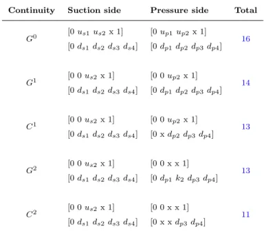
Table 3: Total number of parameters vs continuity at the leading edge
Continuity Suction side Pressure side Total
G0 [0 us1us2x 1] [0 up1up2x 1] 16 [0 ds1ds2ds3ds4] [0 dp1dp2 dp3dp4] G1 [0 0 us2x 1] [0 0 up2x 1] 14 [0 ds1ds2ds3ds4] [0 dp1dp2 dp3dp4] C1 [0 0 us2x 1] [0 0 up2x 1] 13 [0 ds1ds2ds3ds4] [0 x dp2dp3 dp4] G2 [0 0 us2x 1] [0 0 x x 1] 13 [0 ds1ds2ds3ds4] [0 dp1k2dp3dp4] C2 [0 0 us2x 1] [0 0 x x 1] 11 [0 ds1ds2ds3ds4] [0 x x dp3dp4]
G1 continuity at the leading edge is achieved if there exists a scalar k1 > 0 192
so that ˙P (0) = k1· ˙S(0). The first derivative of a Bezier curve Q(u) of degree 193 m: 194 Q(u) = m X i=0 Bim(u) · Qi with u ∈ [0, 1] (8)
is given for u = 0 by: 195
dQ(0)
du = m · (Q1− Q0) (9)
which leads to the definition of the point P1 196 P1= S0+ k1· (S0− S1) (10) with 197 k1= dp1 ds1 (11)
If k1= 1, i.e. dp1= ds1, C1 continuity is achieved. 198
199
G2 continuity at the leading edge is achieved if there exists a scalar k2 > 0 200
so that ¨P (0) = k2· ¨S(0). The second derivative of a Bezier curve Q(u) of degree 201
m for u = 0 is given by 202
d2Q(0)
du2 = m(m − 1) · (Q0− 2Q1+ Q2) (12)
which leads to the definition of the point P2 203
P2= (1 + 2k1+ 2k2) · S0− (2k1+ k2) · S1+ k2· S2 (13) If k1= 1 and k2= 1, C2continuity is achieved. Thus, if G2or C2continuity 204
is prescribed, parameters up2 and dp2 are replaced by k2. 205
3. Optimization process 206
The proposed method uses an optimization loop containing three separate 207
blocks (Fig. 3): geometrical modeling, CFD simulation and genetic optimiza-208
tion. 209
3.1. Geometrical modeling 210
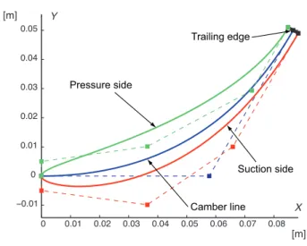
The surface profile is modeled as described in the previous paragraph, i.e. 211
using two Bezier curves for suction and pressure sides. In the example depicted 212
in Fig. 4, two Bezier curves of degree 4 are used to model the suction and 213
pressure sides with a curvature continuity C2 at the leading edge. The trailing 214
edge is sharp and modeled as a straight line. This parameterization leads to 11 215
parameters (Table4). 216
217
The tool path is modeled with the same parameterization than the design 218
approach, that is to say, by means of two Bezier curves of degree 4 with Gn/Cn 219
continuity at the leading edge (Fig. 5, Table5). The degree of the Bezier curves 220
has been chosen to be consistent with the maximum degree of polynomial curves 221
Design parameterization Geometry Meshing CFD computation Post-processing Assessment Genetic Optimization Optimal design *.Step Toolpath parameterization Machining simulation Geometry transfert Matlab ANSYS Matlab Pre-processing icemcfd cfx5pre cfx5solve cfx5post OR
Figure 3: Optimization process
Table 4: C2 example design parameters
Camber line Suction side Pressure side
L 0.1 m us2 0.3 dp3 0.025 m α 30◦ ds1 0.005 m dp4 0.002 m β1 0◦ ds2 0.015 m β1 60◦ d s3 0.045 m ds4 0.002 m
a numerical controller could interpolate, which is equal to 5 for a Siemens 840D 222
[27]. In this way, the proposed design process ensures a full polynomial model 223
from design to manufacturing without any geometric approximation. 224
0 0.01 0.02 0.03 0.04 0.05 0.06 0.07 0.08 0 0.01 0.02 0.03 0.04 0.05 Camber line Suction side Pressure side Trailing edge Y X [m] [m]
Figure 4: C2design example
The first control point of both curves at the leading edge is the offset of the 225
origin point of the camber line CL0 along its tangent vector with a magnitude 226
equal to the tool radius. 227
S0= P0= CL0+ R · t (14)
The last control point of both curves at the trailing edge is the offset of the 228
last point of the camber line CL2 along its normal vector with a magnitude 229
greater or equal to the tool radius. 230
S4= CL2+ (R + ds4) · n (15)
231
P4= CL2− (R + dp4) · n (16)
The points describing the blade surface are generated through a kinematical 232
machining simulation. They are defined as points of the envelope surface of the 233
tool movement computed by a N-buffer algorithm [28] (Fig. 6). This consists 234
in computing intersections between the straight lines of the N-buffer with the 235
cylindrical tool. Those points are then used to build the mesh during CFD 236
simulation. 237
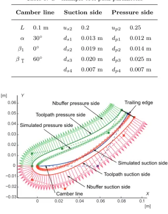
Table 5: G1 example tool path parameters
Camber line Suction side Pressure side
L 0.1 m us2 0.2 up2 0.25 α 30◦ d s1 0.013 m dp1 0.012 m β1 0◦ ds2 0.019 m dp2 0.014 m β1 60◦ ds3 0.020 m dp3 0.025 m ds4 0.007 m dp4 0.007 m 0 0.02 0.04 0.06 0.08 0.1 0 0.01 0.02 0.04 0.05 0.06
Nbuffer suction side Toolpath suction side
Simulated suction side
Camber line
Trailing edge Nbuffer pressure side
Toolpath pressure side Simulated pressure side
[m]
X Y
[m]
Figure 5: G1 tool path example
3.2. CFD simulation 238
The quality of the mesh is an important issue to ensure the quality of the 239
results. In order to obtain accurate results and a robust automatic mesh gener-240
ation during the optimization process, a hybrid (structured/unstructured) mesh 241
is used as shown in Fig. 7. 242
The separation between the two mesh types is performed by the convex 243
envelope of a profile’s offset. This offset is taken with a magnitude equal to 10 244
percent of the chord (L) for the suction and pressure sides and 20 percent for 245
the trailing edge. The convex envelope is used to ensure the robustness of the 246
automatic mesh generation in case of a high curvature blade. 247
The structured mesh is located between the profile and the offset (O-mesh). 248
Figure 6: Blade generated with N-buffer simulation
Figure 7: Hybrid mesh
In this way, the boundary layer effects are well captured due to the better 249
accuracy of this kind of mesh. The unstructured mesh is located between the 250
offset and the boundaries of the fluid domain. Therefore, topological constraints 251
do not depend on the relative position of the profile regarding to the boundaries. 252
The mesh generation is done during the optimization within ANSYS ICEM 253
through a replay script-file written in Tcl/Tk language. The total number of 254
mesh nodes is approximately 100’000 due to the different profiles shapes. 255
The quality of the mesh is checked for the optimal blades at each iteration. 256
The quality criterions for a mesh cell are a minimum angle greater than 15 de-257
grees and a relative Jacobian determinant greater than 0.4 [29]. 258
259
In the present study, the water is assumed as incompressible at constant 260
temperature. The motion of the water is governed by the Reynolds Averaged 261
Navier Stokes (RANS) equations (17) and (18), where p is the static pressure, 262
ν is the kinematic viscosity and Xi= [X, Y, Z] the components of the Cartesian 263
coordinate system. In these equations, the velocity and pressure are split into 264
a mean value and a fluctuating part (19). The Reynolds stresses term defined 265
as ρCi0Cj0 is modelled by the Shear Stress Transport (SST) turbulence model, 266
which is described by Menter et al. [30]. 267 ∂Ci ∂Xi = 0 and ∂C 0 i ∂Xi = 0 (17) 268 ∂Ci ∂t + Cj ∂Ci ∂Xj = −1 ρ ∂p ∂Xi + ν∂ 2C i ∂X2 j −∂C 0 iCj0 ∂Xj . (18) 269 Ci= Ci+ Ci0 and p = p + p 0 (19)
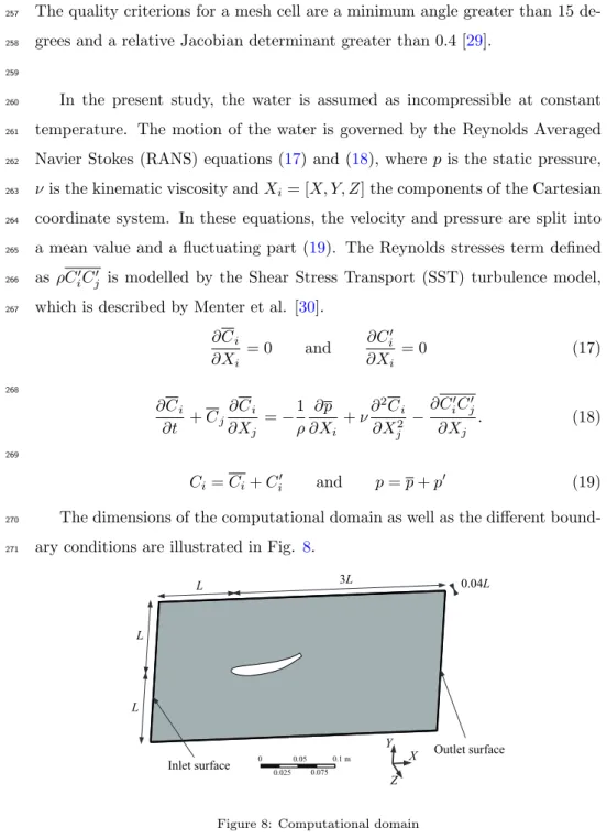
The dimensions of the computational domain as well as the different bound-270
ary conditions are illustrated in Fig. 8. 271 0.1 m 0.05 0.075 0.025 0 L L L 3L 0.04L Inlet surface Outlet surface Z X Y
Figure 8: Computational domain
At the inlet surface, a uniform reference velocity C0 is applied and decom-272
posed as follow: CX = 10 m s−1, CY = 0 m s−1 and CZ = 0 m s−1. Moreover, 273
a turbulent intensity of 5% percent is chosen for the inlet, which corresponds 274
to a medium turbulent intensity. On the outlet surface, a zero average static 275
pressure is imposed. The suction side, pressure side and trailing edge surfaces 276
of the blade are set as no-slip smooth walls. Therefore, the velocity on these 277
surfaces is imposed equal to zero. On the top, bottom and sides surfaces a 278
symmetric boundary conditions is applied [31]. 279
In order to improve the convergence of the computation, the initial conditions 280
for the velocity and pressure are taken from the result of a simulation, which 281
corresponds to the middle of the parameters range (Table6). 282
The software used for the different numerical flow simulation is the com-283
mercial code ANSYS-CFX Release 12.1. The geometry of the computational 284
domain is imported from ANSYS-ICEM. Then, the selected numerical setup 285
for the case study is applied in ANSYS-CFX-Pre. Afterwards, the numerical 286
simulation is performed by ANSYS-CFX-Solver. 287
This solver uses a finite volume discretization of the equations. Conse-288
quently, the continuous value of velocity and pressure of the flow field are dis-289
cretized on each mesh node in order to solve implicitly a system of algebraic 290
equations. The stop criterion for the computation is a maximum residual of 291
5 · 10−6 for each unknown variable or a maximum number of 300 iterations. 292
The results are analyzed with ANSYS-CFX-Post where the interesting values 293
for the optimization process are extracted. In the present study, the extracted 294
values are: the drag force FX, the lift force FY, the maximum velocity value in 295
the computational domain Cmax and the non dimensional wall distance y+. 296
The maximum velocity value in the computational domain is used to eval-297
uate the specific energy losses in the computational domain. Indeed, as these 298
losses are proportional to C22, the minimization of Cmax corresponds to the 299
minimization of the losses. 300
301
The non dimensional wall distance value y+represents the ability of the mesh 302
to take into account the physic of the flow (Eq. 20). This value is proportional 303
to the height of the mesh elements in contact with the blade and to the friction 304
velocity uτ. After each computation, a maximum y+ value below 20 is checked 305
on the profile to simulate the boundary layer behavior and verify the mesh 306 quality. 307 y+= uτ· y ν with uτ = r τp ρ (20) 3.3. Genetic optimization 308
The genetic algorithms are based on the principles of natural genetics and 309
evolution. At each step of the optimization process, the algorithm computes the 310
objectives for each individual. Then, the population is sorted and scaled in order 311
to select the individuals, which will be used to produce the next population. This 312
population is either produced by the mutation of a selected individual (18%) 313
or by the crossover of two selected individuals (80%) and with the two best 314
individuals from the previous iteration (2%) [33]. 315
In the present analysis, the multi-objective optimization process is performed 316
with the global optimization toolbox from Matlab. The size of this population 317
is set to 100 different profiles and the maximum number of iterations is limited 318
to 50, which leads to approximately 5’000 computations per optimization run. 319
The design and tool path parameters are limited by the parameters range 320
given in Table6. Moreover, linear constraints are applied inside the optimization 321
process in order to produce only feasible profile shape (Eq. 21). 322
β1≤ α and α ≤ β1 (21)
In the case of tool path optimization, the curvature radius Rκof both suction 323
and pressure sides has to be greater than the tool radius R to prevent the 324
generation of a loop in the offset profile (Eq. 22). 325
Rκ=
k...Q(u)k3
k ˙Q(u) × ¨Q(u)k and Rκ≥ R (22)
As the purpose of this paper is to compare the design and tool path ap-326
proaches in order to generate a blade, only two objectives are arbitrarily chosen 327
for the present study: maximize FY and minimize Cmax. 328
To decrease the time of the optimization process, the genetic algorithm is 330
used in parallel. Therefore, the simulations of the population are sent to a 331
computational grid to compute several individuals in the same time. 332
4. Numerical investigations 333
Numerical investigations have been conducted for eight different cases, gath-334
ering the two methods and four types of continuity at the leading edge between 335
suction and pressure sides. The range of the geometrical parameters is given in 336
Table6. 337
Table 6: Range of parameters
Parameter Min Max Design tool path
α −5◦ 25◦ x x β1 −20◦ 30◦ x x β1 0◦ 50◦ x x us2 0.01 0.35 x x ds1 0.005 m 0.008 m x o ds1 0.008 m 0.011 m o x ds2 0.005 m 0.015 m x x ds3 0.02 m 0.05 m x x ds4 0.002 m 0.002 m x x up2 0.01 0.35 x x dp1 0.005 m 0.008 m x o dp1 0.008 m 0.011 m o x dp2 0.005 m 0.015 m x x dp3 0.02 m 0.05 m x x dp4 0.002 m 0.002 m x x R 0.005 m 0.005 m o x
For each case study, ten Intel Xeon CPU at 3.00 GHz with eight cores and 338
8 GB of memory are used in parallel during the genetic optimization and each 339
numerical simulation is carried out on four cores. The mean computing time 340
for the simulation of an individual is ten minutes, which leads to an averaged 341
time of one hour per iteration. 342
The objectives are maximization of the lift FY and minimization of the 343
maximal velocity Cmax. The resulting values for the eight cases are gathered 344
in Table 7. Moreover, lift coefficients CL and pressure coefficient Cp,min have 345
been calculated to non-dimensionalize the results. 346 CL= FY ρ ·C02 2 · 0.04L2 and Cp,min= 1 − C2 max C2 0 (23) The magnitude of lift FY and maximum velocity Cmax are approximately 347
the same for both methods and for the different levels of continuities (Table 348
7). However, in the C2 case, the maximum lift is lower by about 15% for both 349
design and tool path approaches. This is because the C2 continuity constraint 350
at the leading edge blocks the first three control points of the pressure side 351
(P0, P1, P2), thereby reducing the degrees of freedom for the generation of the 352
blades. 353
The lift difference between the two methods is always lower than 4%. This 354
is not significant because it has the same order of magnitude as the amplitude 355
of lift fluctuation (±5 N). Indeed, the high curvature profiles generate vortices 356
shedding, which induces a fluctuating lift value during the computation despite 357
the use of a steady solver. Moreover, the differences in the optimization results 358
are likely well within the errors introduced by the RANS model for the complex 359
flows over such blades. 360
The maximal velocity Cmax (or the pressure coefficient Cp,min) is always 361
greater for the tool path method because the curvature radius at the leading 362
edge is imposed by the choice of parameters ds1and ds2. Indeed, if these param-363
eters are too small, the radius of curvature of the generated tool path is lower 364
than the tool radius and the N-buffer simulation is not allowed. The choice of 365
the range of these parameters (Table6) may have been too conservative result-366
ing in more flattened edges, generating slightly higher speed along the profile. 367
368
Since there are two different objectives in the optimization, the Pareto fronts 369
Table 7: Optimisation results
Case Max |FY| Max CL Min Cmax Min |Cp,min|
[N] [-] [m s−1] [-] G1Design 84.14 4.20 12.15 0.48 G1Tool path 88.16 4.41 12.25 0.50 C1Design 87.00 4.35 11.66 0.36 C1Tool path 84.30 4.21 12.08 0.46 G2Design 88.00 4.40 11.73 0.38 G2Tool path 84.74 4.23 12.49 0.56 C2Design 78.02 3.90 11.73 0.37 C2Tool path 76.40 3.82 12.80 0.64 −5 −4 −3 −2 −1 0 1 −5 −4 −3 −2 −1 0 1 −16 −16 −16 −14 −12 −10 −8 −6 −4 −2 0 Design − G
1 Continuity Design − C1 Continuity
CL (lift coefficient) CL (lift coefficient)
CP (pressure coefficient) −5 −4 −3 −2 −1 0 1 −14 −12 −10 −8 −6 −4 −2 0 −16 −14 −12 −10 −8 −6 −4 −2 0 CP (pressure coefficient) Design − G2 Continuity −5 −4 −3 −2 −1 0 1 −14 −12 −10 −8 −6 −4 −2 0 −16 Design − C2 Continuity −5 −4 −3 −2 −1 0 1 −14 −12 −10 −8 −6 −4 −2 0
Toolpath − G1 Continuity Toolpath − C1 Continuity
−5 −4 −3 −2 −1 0 1 −16 −16 −14 −12 −10 −8 −6 −4 −2 0 CL (lift coefficient) Toolpath − G2 Continuity −5 −4 −3 −2 −1 0 1 −14 −12 −10 −8 −6 −4 −2 0 −16 CL (lift coefficient) Toolpath − C2 Continuity −5 −4 −3 −2 −1 0 1 −14 −12 −10 −8 −6 −4 −2 0
Figure 9: Pareto fronts
for the eight cases have been plotted on Fig. 9. It shows that the Pareto fronts 370
resulting from the optimization of the two criterions CL and Cp,min have the 371
same shape and are divided into two zones. 372
The Pareto fronts for the G1 case with design and tool path approaches 373
have been illustrated in Fig. 10 and Fig. 11. Six points on each Pareto front 374
have been chosen and their hydraulic properties have been highlighted. These 375
points are as near as possible for both cases but can’t be exactly identical. 376
The geometry of the blades corresponding to the selected hydraulic properties 377
are presented respectiviely in Fig. 12 and Fig. 13. Results show that there 378
are two different families of blade geometry, which depends strongly on the 379
angles that define the camber line (α, β1 and β1). The geometries created by 380
the conventional approach and the proposed one are similar. Slender blades 381
generate slow velocity profiles whereas curved blades generate high lift values 382
which is coherent with the theory. Both approaches lead to this behavior, which 383
proves that the proposed approach is consistent. 384
−5 −4 −3 −2 −1 0 1 −16 −14 −12 −10 −8 −6 −4 −2 0 X = −2.142 Y = −2.442 Cl (lift coefficient) X = −1.045 Y = −0.957 X = −0.390 Y = −0.703 X = −2.007 Y = −2.16 X = −3.105 Y = −3.263 X = −4.185 Y = −5.319 Cp (pressure coefficient )
Figure 10: Pareto front ; design G1 continuity
−5 −4 −3 −2 −1 0 1 −16 −14 −12 −10 −8 −6 −4 −2 0 CL (lift coefficient) Cp (pressure coefficient) X = −4.406 Y = −5.134 X = −3.081 Y = −3.17 X = −2.25 Y = −2.753 X = −1.056 Y = −0.950 X = −2.017 Y = −2.079 X = −0.371 Y = −0.677
0 0.01 0.02 0.03 0.04 0.05 0.06 0.07 0.08 0.09 0.1 −0.02 −0.01 0 0.01 0.02 0.03 0.04 0.05 −0.390 ; −0.703 −1.045 ; −0.957 −2.142 ; −2.442 −3.105 ; −3.263 −4.185 ; −5.319 −2.007 ; −2.16 Y X [m] [m]
Figure 12: Geometries on Pareto front ; design G1continuity
0 0.01 0.02 0.03 0.04 0.05 0.06 0.07 0.08 0.09 0.1 −0.02 −0.01 0 0.01 0.02 0.03 0.04 0.05 −0.371 ; −0.677 −1.055 ; −0.950 −2.249 ; −2.753 −3.081 ; −3.169 −4.405 ; −5.133 −2.017 ; −2.079 Y X [m] [m]
5. Conclusions 385
In this paper, a different approach to design hydrodynamic profiles has been 386
developed. This approach is based on the definition of a tool path such that 387
the envelope of the movement of the tool optimizes one or more hydrodynamic 388
criteria. A unified parametric model to design the blades for both approaches 389
(design and tool path) was proposed as well as a robust automatic meshing 390
strategy to mesh the fluid domain based on different blade geometries. 391
Overall, the results show that the proposed approach can generate geome-392
tries whose performances are comparable to the ones obtained by the classical 393
approach. The advantage is that these performances are not degraded because 394
the same polynomial curves would be used from the design stage to the ma-395
chining stage without modifications in the post-processor or in the NC unit. 396
Polynomial format ensures the smoothness of the trajectory, which is one of 397
the parameters required to provide a good surface finish. To enhance the op-398
timization, machining phenomena such as dynamical behavior of the machine 399
tool could be introduced in the machining simulation. 400
The method was validated on a 2D example. The next step is the design and 401
manufacture of impellers, usually designed with non-developable ruled surfaces, 402
which are impossible to machine in 5-axis flank milling without geometrical 403
deviations. However, the large number of parameters to control the geometry 404
of such complex blades suggests to use faster optimization technics than genetic 405
algorithms. 406
Nomenclature 407
Geometric parameters
m Degree of the curve [−]
u Curvilinear abscissa [−]
Bim(u) Bernstein polynomial i [−]
Q(u) Bezier curve [−]
Qi Control point i [−]
β1, β1 Inlet, outlet angle [◦]
L Chord length [m]
α Chord angle [◦]
CL(u) Camber line function [m]
CLi Camber line control point i [m]
n Vector normal to camber line [m]
t Vector tangent to camber line [m]
S(t), P (t) Suction, pressure side function [m]
Si, Pi Control point i [m]
usi, upi Control points abscissa i [−]
dsi, dpi Control points distance i [m]
Gn, Cn Continuity degree n [−]
kn Gn/Cn continuity parameter [−]
R Tool radius [m]
Rκ Curvature radius [m]
X∗
d, Xt∗ Optimal design, optimal tool path [−] 408
CFD parameters
X, Y , Z Cartesian component [m]
Xi Cartesian component i [m]
C Absolut velocity [m s−1]
Ci Absolut velocity component i [m s−1]
C0 Reference velocity at inlet [m s−1]
p Static pressure [Pa]
ρ Density [kg m−3]
ν Kinematic viscosity [m2s−1]
FX, FY drag, lift force [N]
y+ Wall distance [−]
τp Wall shear stress [P a]
CL Lift coefficient [−]
Cp Pressure coefficient [−]
409
Abbreviations
CAD Computer Aided Design
CAM Computer Aided Manufacturing
CFD Computer Fluids Dynamics
FEA Finite Element Analysis
GSO Global Shape Optimization
LE Leading Edge
NS Navier Stokes
NC Numerical Controllers
RANS Reynolds Averaged Navier Stokes
SID Shape Inverse Design
SST Shear Stress Transport
TE Trailing Edge
References 411
[1] B.K. Choi , R.B. Jerard. Sculptured surface machining, theory and appli-412
cations. Dordrecht: Kluwer Academic Publishers, 1998. 413
[2] C. Lartigue, F. Thiebaut, T. Maekawa, CNC tool path in terms of B-spline 414
curves, Computer-Aided Design 2001;33:307-319. 415
[3] Cheng, M.-Y., Tsai, M.-C., Kuo, J.-C., Real-time Nurbs command genera-416
tors for CNC servo-controllers, International Journal of Machine Tools and 417
Manufacture 2002;42(7):801-813. 418
[4] E. Duc, C. Lartigue, C. Tournier and P. Bourdet, A new concept for the 419
design and the manufacturing of free-form surfaces: the machining surface. 420
CIRP Annals - Manufacturing Technology 1999;48(1):103-106. 421
[5] H. Tonshoff, N. Rackow, Optimal tool positioning for five-axis flank milling 422
of arbitrary shaped surfaces, Annals of the German Academic Society for 423
Production Engineering (WGP) 2000;7(1): 57-60. 424
[6] C. Menzel, S. Bedi, S. Mann, Triple tangent flank milling of ruled surfaces, 425
Computer-Aided Design 2004;36(3):389-296. 426
[7] J. Senatore, F. Monies, J.-M. Redonnet, W. Rubio, Analysis of im-427
proved positioning in five-axis ruled surface milling using envelope surface, 428
Computer-Aided Design 2005;37(10):989-998. 429
[8] P.-Y. Pechard, C. Tournier, C. Lartigue, and J.-P. Lugarini. Geometrical 430
deviations versus smoothness in 5-axis flank milling. International Journal 431
of Machine Tools and Manufacture 2009;49(6):454-461. 432
[9] C. Lartigue, E. Duc, A. Affouard, Tool path deformation in 5-axis milling 433
using envelope surface, Computer-Aided Design 2003;35(4):375-382. 434
[10] L. Zhu, G. Zheng, H. Ding, and Y. Xiong. Global optimization of tool path 435
for five-axis flank milling with a conical cutter. Computer-Aided Design 436
2010;42(10):903-910. 437
[11] J. Chaves-Jacob, G. Poulachon, and E. Duc. New approach to 5-axis 438
flank milling of free-form surfaces: Computation of adapted tool shape. 439
Computer-Aided Design 2009;41(12):918-929. 440
[12] H. Gong, F. Z. Fang, X. T. Hu, L.-X. Cao, and J. Liu. Optimization of 441
tool positions locally based on the bceltp for 5-axis machining of free-form 442
surfaces. Computer-Aided Design 2010;42(6):558-570. 443
[13] T. Korakianitis and G. Pantazopoulos. Improved turbine-blade design tech-444
niques using 4th-order parametric-spline segments. Computer-Aided De-445
sign 1993;25(5):289-299. 446
[14] B. Dennis, G. Dulikravich, and Z.-X. Han. Constrained shape optimization 447
of airfoil cascades using a navier-stokes solver and a genetic/sqp algorithm. 448
In ASME, International Gas Turbine and Aeroengine. Congress and Exhi-449
bition, Indianapolis, USA, 1999. 450
[15] W. S. Ghaly and T. T. Mengistu. Optimal geometric representation of 451
turbomachinery cascades using nurbs. Inverse Problems in Science and En-452
gineering 2003;11(5):359-373. 453
[16] L. Ferrando, J.-L. Kueny, F. Avellan, C.Pedretti, and L. Thomas. Surface 454
parameterization of a francis runner turbine for optimum design. In 22nd 455
IAHR Symposium on Hydraulic Machinery and Systems, 2004. 456
[17] L. Ferro, L. Gato, and A. Falcao. Design and experimental validation of 457
the inlet guide vane system of a mini hydraulic bulb-turbine. Renewable 458
Energy 2010;35(9):1920-1928. 459
[18] I. Abbott and A. Doenhoff. Theory of wing sections: including a summary 460
of airfoil data. Dover books on physics and chemistry. Dover Publications, 461
1959. 462
[19] D. Bonaiuti, A. Arnone, M. Ermini, and L. Baldassarre. Analysis and op-463
timization of transonic centrifugal compressor impellers using the design of 464
experiments technique. Journal of Turbomachinery 2006;128(4):786-797. 465
[20] G. N. Koini, S. S. Sarakinos, and I. K. Nikolos. A software tool for para-466
metric design of turbomachinery blades. Advances in Engineering Software 467
2009;40(1):41–51, 1. 468
[21] L. Pritchard. An eleven parameter axial turbine airfoil geometry model. In 469
ASME 1985;85-GT-219. 470
[22] S. Pierret and R. A. Van den Braembussche. Turbomachinery blade de-471
sign using a navier-stokes solver and artificial neural network. Journal of 472
Turbomachinery 1999;121(2):326–332. 473
[23] J. M. Anders, J. Haarmeyer, and H. Heukenkamp. A parametric blade 474
design system (part i + ii) Von Karman Institut lecture serie1, 2008. 475
[24] D. Buche, G. Guidati, and P. Stoll. Automated design optimization of 476
compressor blades for stationary, large-scale turbomachinery. ASME Con-477
ference Proceedings 2003;(36894):1249-1257. 478
[25] K. C. Giannakoglou. Design of optimal aerodynamic shapes using stochas-479
tic optimization methods and computational intelligence. Progress in 480
Aerospace Sciences 2002;38(1):43-76. 481
[26] S. Goel. Turbine airfoil optimization using quasi-3d analysis codes. Inter-482
national Journal of Aerospace Engineering, 2009. 483
[27] Siemens. www.automation.siemens.com/doconweb, Sinumerik
484
840D/840Di/810D user, Programming Manual Job planning, 2010. 485
[28] R. Jerard, R. Drysdale, K. Hauck, B. Schaudt, and J. Magewick. Meth-486
ods for detecting errors in numerically controlled machining of sculptured 487
surfaces. IEEE Computer Graphics and Applications 1989;9(1):26–39. 488
[29] ANSYS ICEM CFD 12.1. Help Manual, 2009. 489
[30] F. R. Menter, M. Kuntz, R. Langtry. Ten years of industrial experience 490
with the SST turbulence model. Begell House Inc, 2003. 491
[31] ANSYS CFX-Solver 12.1. Theory Guide, 2009. 492
[32] I. L. Ryhming. Dynamique des fluides. 2nd Edition, Presses Polytechniques 493
et Universitaires Romandes, 2004 494
[33] U. Maulik, S. Bandyopadhyay, A. Mukhopadhyay. Multiobjective genetic 495
algorithms for clustering. Springer, 2011 496