An assessment of body force representations for compressor stall simulation
Texte intégral
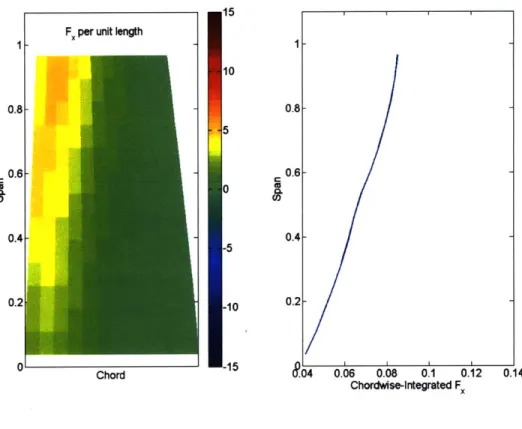
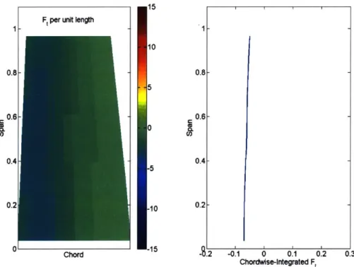
Figure
![Figure 1-1: Typical spike and modal stall inception [1]](https://thumb-eu.123doks.com/thumbv2/123doknet/14105606.466038/13.918.203.695.220.918/figure-typical-spike-modal-stall-inception.webp)
![Figure 1-2: Dependence of stall inception type on occurrence of critical rotor incidence [1]](https://thumb-eu.123doks.com/thumbv2/123doknet/14105606.466038/14.918.179.746.241.876/figure-dependence-stall-inception-occurrence-critical-rotor-incidence.webp)


Documents relatifs
This question, however, will not be elucidated because we prove in Section 4 that the bulk diffusion coefficient is smooth up to the boundary.. Consider the resolvent
We argue that in the context of monitoring, the definition of sensing cost should consider only computations that satisfy the property, and we study the complexity of computing
prolongeant la détention provisoire de toutes les personnes dont le titre de détention devait prendre fin, sans prendre en considération la situation personnelle
numerical simulations give a good agreement with the experimental data with the least good agreement for the EARSM turbulence model due to the size of the recirculation zone which
Hybrid centrifugal spreading model to study the fertiliser spatial distribution and its assessment using the transverse coefficient of variation... Hybrid centrifugal spreading model
In this article we consider the inverse problem of determining the diffusion coefficient of the heat operator in an unbounded guide using a finite number of localized observations..
Notre enquête est une étude pilote dans notre royaume qui vise à explorer l’opinion des anatomopathologistes marocains à propos de l’imagerie numérique dans la pratique de
Maximum pressure values (N/cm 2 ) as monitored during the first and the fifth hippotherapy lesson (Lesson = received hippotherapy lesson; RR = contact of rear right limb,
