HAL Id: hal-01464151
https://hal-amu.archives-ouvertes.fr/hal-01464151
Submitted on 10 Feb 2017
HAL is a multi-disciplinary open access
archive for the deposit and dissemination of
sci-entific research documents, whether they are
pub-lished or not. The documents may come from
teaching and research institutions in France or
abroad, or from public or private research centers.
L’archive ouverte pluridisciplinaire HAL, est
destinée au dépôt et à la diffusion de documents
scientifiques de niveau recherche, publiés ou non,
émanant des établissements d’enseignement et de
recherche français ou étrangers, des laboratoires
publics ou privés.
Distributed under a Creative Commons Attribution| 4.0 International License
Gyrification Indices
Hamed Rabiei, Frédéric Richard, Olivier Coulon, Julien Lefèvre
To cite this version:
Hamed Rabiei, Frédéric Richard, Olivier Coulon, Julien Lefèvre. Local Spectral Analysis of the
Cerebral Cortex: New Gyrification Indices. IEEE Transactions on Medical Imaging, Institute of
Electrical and Electronics Engineers, 2017, 36 (3), pp.838 - 848. �10.1109/TMI.2016.2633393�.
�hal-01464151�
Local Spectral Analysis of the Cerebral Cortex: New Gyrification
Indices
Hamed Rabiei
1,2,3, Fr´ed´eric Richard
3, Olivier Coulon
1,2, and Julien Lef`evre
1,21Institut de Neurosciences de la Timone, Aix-Marseille Universit´e, CNRS, UMR7289, Marseille, France 2Aix-Marseille Univ, CNRS, LSIS, Marseille, France
3Aix-Marseille Univ, CNRS, Centrale Marseille, I2M, Marseille, France
Gyrification index (GI) is an appropriate measure to quantify the complexity of the cerebral cortex. There is, however, no universal agreement on the notion of surface complexity and there are various methods in literature that evaluate different aspects of cortical folding. In this paper, we give two intuitive interpretations on folding quantification based on the magnitude and variation of the mean curvature of the cortical surface. We then present a local spectral analysis of the mean curvature to introduce two local gyrification indices that satisfy our interpretations. For this purpose, the graph windowed Fourier transform is extended to the framework of surfaces discretized with triangular meshes. An adaptive window function is also proposed to deal with the intersubject cortical size variability. The intrinsic nature of the method allows us to compute the degree of folding at different spatial scales. Our experiments show that while more classical surface area-based GIs may fail at differentiating deep folds from very convoluted ones, our spectral GIs overcome this issue. The method is applied to the cortical surfaces of 124 healthy adult subjects of OASIS database and average gyrification maps are computed and compared with other GI definitions. In order to illustrate the capacity of our method to capture and quantify important aspects of gyrification, we study the relationship between brain volume and cortical complexity, and design a scaling analysis with a power law model. Results indicate an allometric relation and confirm the well-known observations that larger brains are more folded. We also perform the scaling analysis at the vertex level to investigate how the degree of folding varies locally with the brain volume. Results reveal that in our healthy adult brain database, cortical regions which are the least folded on average show an increased folding complexity when brain size increases.
Index Terms—Brain folding, gyrification index, spectral analysis, mean curvature, windowed Fourier transform, allometric relation
I. INTRODUCTION
The process of folds appearing on the cerebral cortex is called gyrification. It occurs mostly during the second half of fetal life but continues changing slightly the shape of the folds during post-natal life [1]–[4]. Morphometric parameters of the cerebral cortex such as volume, surface area, sulcal depth, curvature and gyrification index (GI) are commonly used to quantify this gyrification process. Among these, GI is a direct measure that attempts to quantify the degree of folding of the cerebral cortex. It provides valuable information about changes occurring on a brain surface during development, aging, and disease [4]–[10]. In this paper, we propose two new GIs that take into account two different aspects of folding quantification.
Existing GI definitions in the literature, from a general point of view, may be categorized in two classes: surface area (perimeter)-based methods [5]–[7], [11]–[14] and curvature-based methods [10], [15]–[17].
Methods in the first category compute the gyrification index as a ratio between the local area (perimeter) of the cortical surface and that of a reference surface. For instance, Toro et
al. [5] defined a local GI as a ratio between the area of the pial
surface contained in a spherical neighbourhood of each cortical point and the area of the great disc of the sphere. Schaer et al. [6] proposed a ratio between the area of a region of interest, determined by intersection of a sphere with the convex hull
Copyright (c) 2010 IEEE. Personal use of this material is permitted. However, permission to use this material for any other purposes must be obtained from the IEEE by sending a request to [email protected].
Corresponding author: H. Rabiei (email: [email protected]).
of the cortical surface, and that of the corresponding patch on the pial surface as a local GI. The locality of results of those methods depends on the radius of the spherical neighbourhood. In order to deal with the size variability in a database (e.g. fetal brains), the radius would have to be adapted for each subject but no intrinsic strategy exists to choose an appropriate one. To tackle this issue, Lef`evre et al. [4] proposed to adapt the radius r so that it equals a fraction of the brain length in the rostro-caudal direction. Another drawback of those methods is that if there are two cortical regions with equal areas inside the sphere, one contains deep folds and the other one is formed by shallower but more oscillating folds, these methods give equal GI value to both regions. This means that they may not distinguish between deep folds and oscillating folds with equal surface areas. For instance, Schaer’s and Toro’s methods both give high GI values to deep folds like the insula and the central sulcus. In a more general way, both methods tend to produce similar GI maps; see [5, Fig. 5a-c] and [6, Fig. 4].
Methods in the second category rely on the curvature and its derivatives e.g. the mean curvature. The mean curvature is a geometric tool that measures locally how a surface is deviated from being flat. It defines a function on the cerebral cortex and assigns positive values to points on gyri and negative values to points on sulci [18]. The mean curvature map, however, is too local to deliver a helpful insight into the surface folding [15]. Moreover, as Shimony et al. [10] have recently shown, the curvature and its derivatives (e.g. the mean curvature, Gaussian curvature, shape index etc.) by themselves may not be able to discriminate between normal and aberrant cortical development. Nevertheless, the curvature
contains useful information about the surface bending. Luders
et al. [15] defined a local GI by smoothing the magnitude of
the mean curvature. Kim et al. [16] has recently proposed a new GI by quantification of the shape index variance in a local region. Due to the heat kernel smoothing procedure used in these methods, they are likely to miss some folding features at fine scales.
Recently, the spectral analysis of mean curvature based on the spectrum of Laplace-Beltrami operator has been used to study cortical folding. By binning the global frequency distribution in several frequency bands and computing the dominant and the determinant bands, Germanaud et al. [19] derived two metrics of folding that can discriminate primary, secondary and tertiary folds. In a work by Shishegar et al. [17], a new GI has been proposed by computing the weighted differential mean curvature along the level sets of the first non-trivial Laplace-Beltrami eigenfunction. This method focuses mainly on sulcal bending and assigns the lowest values to points on gyri.
The above-mentioned methods have different implicit in-terpretations of the concept of ”surface complexity” that underlies GIs and sometimes their findings lack consistency [20]. In this paper, we propose an explicit interpretation of this notion in an intuitive way that relies on the surface bending properties :
In a neighbourhood around each point of the cerebral cortex, the surface complexity is quantified by
I. the magnitude of sulcal/gyral bending, or II. the spatial frequency of sulcal/gyral bends.
Due to the natural link between the surface bending and the mean curvature, the above interpretations mean that in a highly folded region, (I) the magnitude or (II) the variations of the mean curvature are higher in comparison to other regions. Given those interpretations, we propose two novel local GIs, called spectral gyrification index (sGI) and weighted spectral gyrification index (wGI) based on a local spectral analysis of the mean curvature. These GIs are scale invariant and are computed directly on the cortical surface with neither of them requiring a reference surface nor a smoothing procedure. While sGI gives information about the magnitude of the mean curvature in a neighbourhood around each point on the cortical surface (Interpretation I), wGI takes into account the spatial frequency of folds in that neighbourhood (Interpretation II). The intrinsic nature of the method enables us to compute the surface complexity at different spatial scales. Moreover, in contrast to the surface area-based GIs, the proposed indices are able to disentangle the effect of depth on folding quantifi-cation. Finally, the issue of inconsistent analysis arising from the inter-subject brain size variability is also addressed by in-troducing an adaptive neighbourhood. To our best knowledge, the GIs proposed by Li et al. [7] and Kim et al. [16] are the only ones that tried to tackle this issue before.
In the following, we present in Section II a local spectral analysis method based on the graph windowed Fourier trans-form of the mean curvature. This analysis is used to define the two gyrification indices, sGI and wGI, together with their properties. The method is applied to some synthetic surfaces
and real data in Section III. Finally, we discuss the results and the specificities of our method, followed by a conclusion.
II. METHOD
In this section, we use a local spectral analysis of the cortical surface mesh to define the mesh windowed Fourier transform of the mean curvature function and we show that it can be used to define two new gyrification indices. Spec-tral methods for surface analysis rely mainly on eigenvalues and/or eigenfunctions of an operator defined on the surface. For example, for a Riemannian surface, the eigenfunctions of the Laplace-Beltrami operator serve as bases for Fourier transforms. The idea has been extended to triangular meshes modelling surfaces to analyse their structural properties; see [21] for a comprehensive survey on this topic. Here, we use such eigenfunctions to define a mesh windowed Fourier transform and provide an explicit access to the local frequency components of the mean curvature of the cortical surface.
A. Mesh Fourier Transform
For a compact Riemannian manifold S as a surface in IR3, one can consider a set of square integrable functions defined on the surface: L2(S) = {u ∶ S → IR∣ ∫
Su2 < ∞}. The Laplace-Beltrami operator ∆, associated with the surface S, is defined as a generalization of the Laplacian operator in Euclidean space to Riemannian manifolds. The spectrum of this operator {(λi, ui) ∈ IR+× L2(S), i = 1, 2, . . .} is
generated by solving the differential eigenvalue problem of ∆: ∆ui= −λiui in which λi and ui are called the ith-eigenvalue
and eigenfunction of ∆ [22]. The spectral theory based on the Laplace-Beltrami spectrum can be used to obtain a new representation of the spaceL2in the so called spectral domain. In practice, the differential eigenvalue problem of ∆ is usually solved on a triangulated surface by numerical methods.
Formally, let G = {V, E} be a triangular mesh mod-elling the surface S where V is the set of vertices, V = {P1, P2, . . . , PN}, ∣V ∣ = N < ∞ and E is the set of edges. By
using the linear finite element method (FEM) [23], the above-mentioned differential eigenvalue problem is discretized to the following algebraic generalized eigenvalue problem
Aχ= λBχ, (1)
where A and B are N× N sparse matrices with the following elements: A(i, j) =⎧⎪⎪⎪⎨⎪⎪ ⎪⎩ cot αij+cot βij 2 if (i, j) ∈ E, − ∑k∈N (i)A(i, k) if i= j, 0 o.w. (2) and B(i, j) =⎧⎪⎪⎪⎪⎨ ⎪⎪⎪⎪ ⎩ ∣t1∣+∣t2∣ 2 if (i, j) ∈ E, ∑k∈N (i)∣tk∣ 6 if i= j, 0 o.w. (3)
where αij and βij are the angles opposite to the edge PiPj
in two triangles t1 and t2 sharing this edge,∣tk∣ indicates the
area of the triangle tk andN (i) denotes the index set of all
positive definite and defines the so called B-inner product in IRN:
∀f, g ∈ IRN, ⟨f, g⟩
B= ftBg. (4)
Solutions of the discrete eigenvalue problem (1) are nonneg-ative real eigenvalues 0 = λ1 < λ2 ≤ . . . ≤ λN and a set of
eigenvectors{χj, j= 1, 2, . . . , N} in IRN which are
orthonor-mal with respect to B-inner product i.e.⟨χi, χj⟩B= δij where δij is Kronecker delta.
The bases of the Fourier transform in continuous domain are complex exponential functions which are the eigenfunctions of the Laplace-Beltrami operator. Inspired by this fact, the eigenvectors of the discretized Laplace-Beltrami operator serve as Fourier atoms on the triangulation [24]. Given a function
f defined on the vertices of triangulation, Fourier transform
coefficients of f are given by the set { ˆf(l) ∶= ⟨f, χl⟩B, l =
1, 2, . . . , N}. This set is a representation of function f in the spectral domain and gives the frequency distribution of this function. In this setting, the Parseval’s identity is
⟨f, g⟩B= ⟨ ˆf , ˆg⟩, (5)
where ⟨., .⟩ denotes the Euclidean inner product. It yields ∥f∥B= ∥ ˆf∥2 where∥.∥B is the norm induced by the B-inner
product.
B. Local Mesh Fourier Transform
The mesh Fourier transform described in Section II-A gives a global frequency distribution of a function f . In other words, it is not able to provide information about the frequencies of f in a spatial neighbourhood. In continuous domain, the windowed Fourier transform was introduced in order to find the local frequency distribution of a function [25]. This trans-form gives local intrans-formation about a function simultaneously in spatial and frequency domains.
Shuman et al. [26] have recently extended this transform to graph setting which enables us to do a ”vertex-frequency analysis”. The general idea of this method is to localize a function defined on the vertices of a graph around a vertex by a translated window function and then, compute the graph Fourier transform of this localized function. In this paper, we extend the method to the mesh framework by using the mesh Fourier transform that is aware of the surface geometry.
Since a mesh is a special kind of a graph, embedded in a surface, one may argue that the graph spectral theory tools can be applied on a mesh without any adaptation. In general, it is true but unlike the graph Laplacian in which only the connectivity of vertices are considered, the geometric (FEM) Laplacian takes into account geometric properties of the surface. Equations (2) and (3) show how the geometry of neighbouring triangles on the mesh contributes to the defini-tion of Laplacian operator. More discussions and comparisons between the graph Laplacian and the geometric Laplacian can be found in [21], [23], [24], [27]–[29].
1) Window function and translation operator
Let f ∶ V → IR be a function defined on the vertices of a triangulation (e.g. the mean curvature). To localize this function around a specific vertex, we need a window function with local support and a translation operator to move the
window function to that specific vertex. Following [26], we consider the window function
ˆ
g(l) = C exp(−τλl), (6)
defined in the spectral domain. In this formula, τ is a pa-rameter which determines the size of the window, λl is the l-th Laplace-Beltrami eigenvalue and C is chosen such that
∥ˆg∥2= 1.
The window size parameter τ sets a locality trade-off between the frequency and spatial domains [26], [30]. By increasing the window size, we will have a wider window in the spatial domain and the function f will be localized in a larger neighbourhood around each vertex. On the other hand, more local frequency distribution of the function in that neighbourhood is obtained. The spread of window function in spatial and frequency domains is measured by the area of the Heisenberg box [31, Section 4.2], [26, Section 6.6]. It is proved that the Gaussian function is the unique window that minimizes the area of the Heisenberg box [31, Theorem 2.5]. Since λl is proportional to the square of the spatial
frequency [32], [33], i.e. λl ∝ ω2l, the window function (6)
corresponds to a Gaussian function in the frequency domain ˆ
g(l) ∝ exp(−τωl2).
The fact that there is no canonical origin and direction on a triangulated mesh makes it difficult to define a translation operator on this mesh. Inspired by the properties of the generalized Fourier transform in continuous domain and the mechanism proposed in [26] for graph setting, the translation operator is defined on a triangulation as (see Appendix A for the details of derivation):
Ti∶ IRN → IRN i= 1, 2, . . . , N, (Tig)(n) ∶= √ N N ∑ l=1 N ∑ m=1 (ˆg(l)B(i, m)χl(m)χl(n)). (7)
The translation operator Ti shifts the center of the window
function to a vertex Pi. Now, by multiplying the function f
by the translated window function Tig, it is localized around
the vertex Pi:
˜
fi(n) = (Tig)(n)f(n), n= 1, 2, . . . , N. (8)
2) Mesh windowed Fourier transform
The mesh windowed Fourier transform coefficients of a function f∈ IRN are defined as the modulation of the localized function ˜fi by Fourier atoms{χk, k= 1, 2, . . . , N}:
Sf(i, k) ∶= ⟨ ˜fi, χk⟩B, (9)
where i = 1, 2, . . . , N is the index of vertex and k is the index of frequency. This gives us a frequency spectrum {∣Sf(i, k)∣2, k= 1, 2, . . . , N} for every vertex P
iof the mesh
which can be seen as the frequency distribution of the function
f in a local neighbourhood around the vertex Pi.
3) Adaptive window function
It is easily seen from Eqs. (1)–(3) that if the surface area is scaled by a factor q2, the eigenvalues are scaled by 1/q2. In this case, due to the definition of the window function (6), the relative spread of window (i.e. the ratio between the region area covered by the window and the surface area) is affected by
(a) (b) (c)
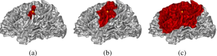
Fig. 1. The spread of the adaptive window function (10) with 3 different window sizes around the yellow vertex on a cortical surface by thresholding the values of the window functions at the same percentage of their maximal values. The red color highlights the window spread around the vertex. (a) A narrow window, with τ = 2e − 4, covers about 1.5% of the surface. (b) A medium window, with τ= 1e−3, covers about 8% of the surface. (c) A wide window, with τ= 5e − 3, covers about 36% of the surface.
the size of the surface. In other words, given a fixed window size τ for the original and the scaled surfaces, the window covers relatively larger space on the smaller surface and vice versa. This leads to an inconsistent large and small scale spectral analysis for small and large surfaces, respectively (see Fig. S1a of supplementary figures).
To keep the relative spread of window constant automat-ically across surfaces (Fig. S1b), we introduce an adaptive window function in which the surface area is incorporated:
ˆ
g(l) = C exp(−τ∣S∣λl), (10)
where∣S∣ denotes the surface area of surface S. Note that by this definition, a dimensionless parameter is obtained inside the exponential. As we will see in Section II-C1, the adaptive window function also plays an important role to derive scale invariant gyrification indices.
In Fig. 1, the spread of the adaptive window function (10) with 3 different window size parameters, τ = 2e − 4, 1e − 3 and 5e− 3 is plotted on a cortical surface around a specific vertex shown as a yellow point on the precentral gyrus. As τ increases, the spread of window in spatial domain increases as well. While the narrow window, τ = 2e − 4, covers a part of a gyrus and/or sulcus, the medium window, τ = 1e − 3, covers several folds and the wide window, τ = 5e−3, covers a big portion of the cortical surface equivalent to a lobe. Tuning the window size parameter τ changes the spatial scale of the analysis.
C. Gyrification Indices
To define gyrification indices that fulfill our interpretations on the surface complexity, stated in Introduction section, we take the mean curvature as a function defined on the vertices of a mesh. By applying the mesh windowed Fourier transform to this function, we will have a frequency spectrum at each vertex Pi of the mesh which consists of the so called
”fre-quency powers” ∣Sf(i, k)∣2, k= 1, 2, . . . , N. The summation of the frequency powers is called the total power (TP) of the frequency spectrum [31]. We proved that the TP of the frequency spectrum of the vertex Piequals to the norm of the
localized mean curvature around this vertex (see Proposition 1 in Appendix B): N ∑ k=1 ∣Sf(i, k)∣2= ∥ ˜f i∥2B. (11)
Due to our first interpretation, in a more folded region, the magnitude of the mean curvature increases. This interpretation, together with Eq. (11), leads to the definition of the first GI:
I. Spectral Gyrification Index (sGI):
sGI(i, S) =
N
∑
k=1
∣Sf(i, k)∣2. (12) In this equation, sGI(i, S) denotes the spectral gyrification index of vertex Pi of surfaceS.
On the other hand, based on our second interpretation, the variation of the mean curvature increases in more folded regions. Since the high variation of a function is encoded in the high frequency band of its frequency spectrum, we give larger weights to higher frequency powers to take into account this interpretation. It brings us the second GI:
II. Weighted Spectral Gyrification Index (wGI):
wGI(i, S) = N ∑ k=1 (λk λ2 ) 2 ∣Sf(i, k)∣2 . (13)
In this equation, the weights are the normalized eigenvalues of the Laplace-Beltrami operator that contain information about the shape of surface [34], [35]. The normalization by the first nonzero eigenvalue λ2removes the effect of the size of surface on weighting [36]. In this definition, both Laplace-Beltrami eigenvalues and eigenvectors are involved.
We proved that
wGI(i, S) = 1
λ2 2
∥L ˜fi∥2B, (14)
where L = B−1A is the Laplace-Beltrami operator (see
Proposition 2 in Appendix B). Since this operator measures how much a function differs at a point from its average value at neighbour points,(L ˜fi)(m) measures the variation of ˜fi at vertex Pm and so, wGI(i, S) sums up all of these variations
of localized f around vertex Pi. 1) Geometric invariance
We now provide some important properties of the proposed GIs. The Laplace-Beltrami spectrum is invariant under isomet-ric transformations. It makes sGI and wGI isometry invariant. Moreover, as demonstrated in Proposition 3 of Appendix B, sGI and wGI are both scale invariant by their constructions.
2) Global GIs
Given a surface mesh with M triangular faces S = {t1, t2, . . . , tM}, GI defines a function on the vertices of this mesh. We define the global GI of surfaceS as the mean value of this function: GI(S) = 1 ∣S∣ M ∑ j=1 1 3 3 ∑ i=1 GIj(i, S)∣tj∣, (15)
where GIj(i, S) denotes the GI value (sGI or wGI) of the i-th
vertex of the face tj and∣tj∣ is the area of tj. It is noteworthy
III. EXPERIMENTS ANDRESULTS
A. Synthetic data
In order to illustrate the efficiency of sGI and wGI for measuring the degree of folding of a surface, and to show the effect of sulcal depth on surface area-based methods, we computed our GIs and Toro’s GI [5] on some synthetic surfaces for which we control the degree of folding.
1) Wavy rectangle
A wavy rectangle in IR3 is created by the equation z = 2 sin(60πx2)/(60πx) where −0.7 ≤ x ≤ 0.7 and 0 ≤ y ≤ 1 with geodesic length equals to 4. This surface is triangulated with
N = 40, 000 equidistant vertices and is shown in Fig. 2a. The
intersection of this surface with the plane y= 0.5 is indicated on the surface by green points and is plotted in Fig. 2b. As we go far from the center to the left or right side of this surface, it becomes more folded i.e. the surface becomes more bended and the spatial frequency of the folds increases. The windowed Fourier transform is applied on the mean curvature of this surface and the spectrogram that consists of the frequency powers ∣Sf(i, k)∣2 is shown in supplemental Fig. S2a (see supplementary figures).
In Fig. 2b, the neighbourhoods of two vertices Pm and Pn
are shown. Obviously, the surface is more folded around Pm
than Pn while there are deeper folds around the latter. The
local frequency spectrums of these vertices are plotted in the supplemental Figs. S2b and S2c that show clearly how higher frequency powers increase in regions with high oscillating folds. The values of sGI, wGI and a surface area-based GI defined by Toro et al. [5] for those vertices are given in Table I for comparison. While sGI and wGI give appropriately higher values to vertex Pm, Toro’s GI gives equal values to both
vertices. It shows that surface area-based GIs may not be able to discriminate between deep folds and complex folds with the same area.
sGI, wGI and Toro’s GI values of the vertices along the green middle line of the wavy surface are plotted in Fig. 2c. The observations clarify that sGI and wGI discriminate efficiently deep folds from complex ones with a clear increase from the center towards the borders whereas Toro’s GI shows high values on the center where there are deep folds.
TABLE I
DIFFERENTGIS FOR VERTICESPmANDPnOF THE WAVY RECTANGLE DEPICTED INFIG. 2B
vertex sGI wGI Toro’s GI
Pm 8.5561e2 2.8090e10 2.2268 Pn 1.8487e2 3.8802e9 2.2271
To elucidate more the effect of the fold depth on the surface area-based GIs, two other surfaces are constructed; see Figs. S3 and S4 of the supplementary figures. These surfaces are designed to study the effect of fold depth and oscillation frequency separately.
B. Real Data
In this section, the proposed method is applied to a real database of cortical surfaces. The gyrification maps of an
(a)
(b)
(c)
Fig. 2. (a) Wavy rectangle in IR3. The ”middle line” on the surface is formed by the vertices lie on the surface with the the same y-coordinate 0.5. (b) The middle line along with zoom on two neighbourhoods around vertices Pm and Pn. (c) Values of Toro’s GI, sGI and wGI of the vertices located on the middle line.
individual subject as well as group average maps across all subjects are presented. The relation between the proposed GIs and the brain volume is also studied.
1) Data and preprocessing
We applied the method to 124 healthy adult subjects from the Open Access Series of Imaging Studies (OASIS) database1. For each subject, three or four T1 anatomical Magnetic Resonance Images (MRIs) had been acquired at in-plane resolution of 1mm× 1mm, slice thickness = 1.25 mm, TR = 9.7 ms, TE = 4 ms, flip angle = 10u, TI = 20 ms, TD = 200 ms. Images of each subject were motion corrected and averaged to create a single image per subject with a high contrast-to-noise ratio.
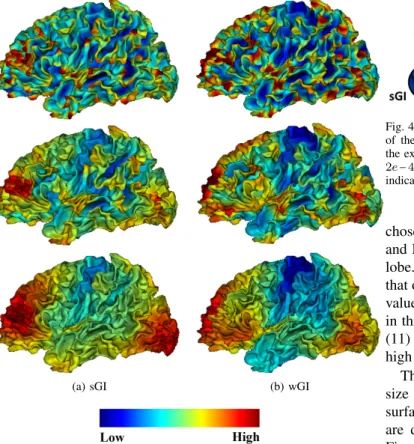
(a) sGI (b) wGI
Fig. 3. The map of gyrification indices (a) sGI and (b) wGI of the left hemisphere of an individual subject from our database at 3 different scales. In the first row τ= 2e − 4, in the second row τ = 1e − 3 and in the third row τ = 5e − 3. The blue and red colors indicate the extremes of low and high degree of folding respectively.
The resulting anatomical MR images were segmented using BrainVISA2. The white matter surface of each hemisphere was then meshed using this software which resulted in triangular meshes with spherical topology and approximately 50,000 nodes depending on the subjects. The Hip-Hop algorithm [37] in BrainVISA was then applied to compute the spherical interindividual correspondence between cortical surfaces.
2) Gyrification maps
The maps of sGI and wGI of a subject from the database are shown in Fig. 3 for 3 different window sizes, τ = 2e − 4, 1e− 3, 5e − 3 associated to very local, medium and wide windows, respectively (see Fig. 1 for window sizes). On this figure, it is shown that the window size parameter τ can be used to control the scale of observations. At τ = 2e − 4, the spatial scale is fine and high values are located mostly on the ridge of complex gyri, while low values are located on the walls of regular sulci. As the window size increases, a more regional effect becomes visible, with a very smooth and low variation map at value τ = 5e − 3, which gives a coarse scale observation of the gyrification.
As it has been discussed in Section II-C, the indices sGI and wGI, based on their constructions, measure complementary properties of surface folding. This is shown in Fig. 4 where the mean curvature of the same cortical surface of Fig. 3 is depicted. Two regions on this surface, R1 and R2, have been
2http://brainvisa.info/
Fig. 4. Zoom on 2 regions, R1 and R2, of the cerebral cortex. The colormap of the cortex encodes its mean curvature (the blue and red colors indicate the extremes of negative and positive values respectively). sGI and wGI (τ= 2e−4) of the regions R1 and R2 are also represented (the blue and red colors indicate the extremes of low and high degree of folding respectively).
chosen. R1 is a sharp spike located on the postcentral gyrus and R2 is a very shallow fold located on the superior parietal lobe. The mean curvature of the region R1 is very high while that of the region R2 varies a lot between positive and negative values. The maps of sGI and wGI of R1 and R2 are shown in this figure (τ = 2e −4). As expected theoretically from Eqs. (11) and (14), sGI gives high value to R1 while wGI assigns high value to R2.
The group average of both GIs in the medium scale (window size τ = 1e − 3) have been computed by using the cortical surface inter-subject matching method, Hip-Hop [37]. Results are depicted on the template cortical surface hiphop1383 in Fig. 5 for the left hemisphere. The average patterns of sGI and wGI represented in this figure are similar to those observable on an individual subject (Fig. 3) which shows that the spatial patterns of the proposed GIs are reproducible across subjects. As Fig. 5a shows, sGI gives higher values to vertices on the prefrontal and occipital lobes, inferior parietal lobe, inferior temporal sulcus and the medial area of the superior parietal cortex. wGI, as shown in Fig. 5b, assigns higher values to the prefrontal lobe, medial part of the occipital lobe and the posterior cingulate gyrus. Some folding is also captured by high wGI values in the insula. We also computed the average GIs of the right hemispheres and by visual inspection, we observed no remarkable difference in gyrification patterns of the left and right hemispheres in the medium scale (see Supplemental Fig. S5).
To compare with our results, the average map of Toro’s GI across all subjects in the database is presented in Fig 5c. This method gives high GI values to deep folds like the central sulcus, the insula, the superior temporal sulcus and the parieto-occipital sulcus.
3) Scaling analysis
Recent studies show that larger brains are more folded [5], [9], [19], [38]. To investigate this phenomenon, the global sGI and wGI of each hemisphere are modelled by the following power law
G= kVα, (16) where G denotes the global gyrification index (sGI or wGI) of a hemisphere computed through Eq. (15), V is the hemispheric volume and k and α are coefficients to be determined. Since
3The hiphop138 template is available at http://www.meca-brain.org/ softwares/hiphop138-cortical-surface-group-template/
(a) sGI
(b) wGI
(c) Toro’s GI
Fig. 5. Average of gyrification indices: (a) sGI and (b) wGI derived from the medium window (τ= 1e−3), and (c) Toro’s GI with spherical neighbourhood radius r= 20 across the left hemispheres of all 124 subjects on the hiphop138 template surface3. The blue and red colors indicate the extremes of low and high degree of folding respectively.
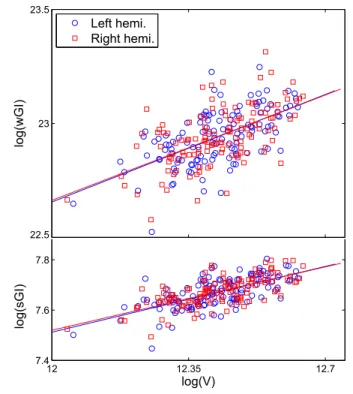
gyrification indices, sGI and wGI, are scale invariant (Propo-sition 3), the scaling exponent coefficient α of the power law (16), under the isometric scaling of brain volume, should equal 0. The hemispheric data along with the fitted power law model in logarithmic scale are represented in Fig. 6. The positive exponent coefficient reveals a positive allometric scaling of gyrification indices with volume. Moreover, it confirms that the larger brains are more folded. The values of the exponent coefficient α of wGI is more than that of sGI (0.67 > 0.37 and 0.66> 0.36 for left and right hemispheres, respectively) while the proportion of the variance of sGI explained by the volume is higher than that of wGI (0.44> 0.36 and 0.47 > 0.34 for left and right hemispheres, respectively). The results also suggest that in the global hemispheric scale, the degree of folding of the left and right hemispheres increase with volume symmetrically.
The above-mentioned results support this hypothesis that the larger brains are more folded but they do not illustrate which cortical regions get more folded in larger brains. To address this question, we perform the allometric analysis (16) at the vertex level. Thanks to the inter-subject matching by Hip-Hop method [37], we are able to find the corresponding
12 12.35 12.7 7.4 7.6 7.8 log(V) log(sGI) 22.5 23 23.5 log(wGI) Left hemi. Right hemi.
Fig. 6. Up: Relationship between the volume (mL) of the left/right hemi-spheres and global wGI (τ= 1e − 3). The fitted line for the left hemisphere is y= 0.67x + 14.57, R2 = 0.36, p < 0.001. The fitted line for the right hemisphere is y= 0.66x + 14.74, R2= 0.34, p < 0.001. Down: Relationship between the volume (mL) of the left/right hemispheres and global sGI (τ= 1e−3). The fitted line for the left hemisphere is y = 0.37x+3.03, R2= 0.44, p < 0.001. The fitted line for the right hemisphere is y = 0.36x + 3.2, R2= 0.47, p < 0.001.
vertices across all subjects. Our method naturally allows us to monitor the changes of the degree of gyrification at different spatial scales. The maps of the significant exponent coefficient
α (p < 0.05, corrected for multiple comparisons using False
Discovery Rate (FDR) [39]) for sGI and wGI of the left hemispheres derived from the medium window (τ = 1e − 3) are represented in Fig. 7. In this figure, the vertices for which
α is not significant are masked by the gray color. Fig. 7 shows
that in the adult population, as brain size increases across subjects, deep folds with low gyrification (represented in blue in Fig. 5a and 5b), such as the central sulcus, the insula, the superior temporal sulcus, or the parieto-occipital sulcus, show the largest increase in folding complexity. We have not observed any vertex with significant negative exponent except in the right hemisphere with the most local window (τ = 2e − 4). In this case, for sGI map, we observed about 0.04% of vertices with significant negative α exponent located on the anterior cingulate and the superior parietal cortices. For wGI, there are only 0.02% of vertices with significant negative
α exponent located on the isthmus cingulate cortex. The
α-maps of the right hemisphere (τ = 1e − 3) are given in Fig. S6 (see supplementary figures).
IV. DISCUSSION ANDCONCLUSION
In this study, we interpreted the cortical surface complexity in two ways that are consistent with the intuitive concept of it.
(a) sGI
(b) wGI
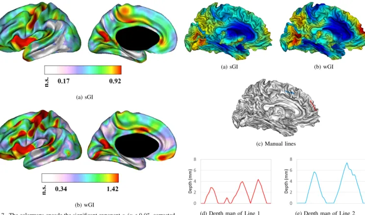
Fig. 7. The colormaps encode the significant exponent α (p< 0.05, corrected for multiple comparisons using FDR) of vertex-wise allometric analysis (16) of gyrification indices (a) sGI and (b) wGI of the left hemisphere derived from the medium window (τ= 1e − 3). The magenta and red colors indicate the extremes of low and high values of α. The regions where α is not significant (n.s.) are masked by gray color. The higher the value of α, the higher the variation of folding with respect to volume.
Based on these assumptions and by applying the local spectral analysis of the mean curvature, we developed a method to estimate locally the degree of folding of the cerebral cortex. The method was applied to a database of 124 healthy adult brains and the results demonstrate that the primary folds like the central sulcus and the insula are less folded than other regions. The central sulcus is a good example since it is a very deep fold but with a high regularity and straight shape where we expect a low measure of folding whereas surface area-based methods usually show high gyrification values (see Fig. 5).
Through some experiments on synthetic surfaces, we clar-ified that surface area-based methods such as Toro’s [5] and Schaer’s [6] GIs may fail to discriminate between deep and complex folds. Indeed, these GIs give higher values to deep folds; see the similar gyrification maps of Toro’s GI [5, Fig. 5a-c] and Schaer’s GI [6, Fig. 4]. To address this issue, Su
et al. [14] proposed to weight the GI by the geodesic sulcal
depth. Nevertheless, we believe that this weighting strategy is in contradiction with the notion of folding. In fact, if a cortical region with deep sulci and another region with shallow sulci have equal areas, the latter region should be more folded to keep the same area as the former one.
As an illustrative example to show how our method dis-criminates between deep and oscillating folds of a cortical surface, the medial face of a subject is considered and its sGI and wGI maps are shown in Fig. 8a and 8b respectively
(a) sGI (b) wGI
(c) Manual lines
(d) Depth map of Line 1 (e) Depth map of Line 2 Fig. 8. Medical view of the map of (a) sGI and (b) wGI of a subject. The blue and red colors indicate the extremes of low and high degree of folding respectively. (c) Two lines with almost equal geodesic length are drawn on the medial prefrontal region (Line 1, red, geodesic length=35.35 mm) and the medial central region (Line 2, blue, geodesic length=34.63 mm). The depth maps of (d) Line 1 and (e) Line 2 show that the frequency of folds in the medial prefrontal region is double of that in the medical precentral region while the depth of folds on the medial prefrontal region is almost half of that in the medial precentral region.
(the lateral maps are shown in the middle row of Fig. 3). Two lines with equivalent geodesic length were drawn on the medial side: line 1 in the medial prefrontal region (red line, geodesic length 35.35 mm) where both GIs show high values, and line 2 in the medial precentral region (blue line, geodesic length 34.63 mm) where both GIs have low values (Fig. 8c). Geodesic sulcal depth on the cortical surface was computed [38] in order to get depth values at each point of both lines and produce depth curves along these lines. These depth curves, plotted in Fig. 8d and 8e, show that the frequency of folds in the medial prefrontal region (Line 1) is double of that in the medial precentral region (Line 2), while the depth of folds on the medial prefrontal region (Line 1) is almost half of that in the medial precentral region. This explains the high values of our gyrification index in the medial prefrontal region: despite an apparent smoothness due to the low sulcal depth, the folding frequency is high.
Another difference between our method and surface area-based methods is that the latter may be not localized enough for some applications. For example, in Fig. 4 of [6], for a small spherical neighbourhood, the most folded region of the cortex is around the Sylvian Fissure and as the size of the neighbourhood increases, the same pattern propagates across the cortex. Therefore, it may fail to catch other folded parts
of the brain, thus affecting the reliability of findings. In our method, by tuning the neighbourhood size, we get the results at different spatial scales, ranging from a very local scale (in order of a part of a sulcus/gyrus) to a more global scale (in order of a lobar cortex); see Figs. 1 and 3.
Despite the differences we highlighted between our method and previous GI definitions, we do think that these previous gyrification indices are still valid but should be considered in the light of their specific interpretations of the notion of ”surface complexity”. Our experiments on synthetic surfaces show that how different interpretations of this notion may lead to different results. Accordingly, a message of this paper is to point out that one should pay attention to this notion and interpret results based on it. Another work on this topic has been done by Awate et al. [20] discussing about the different meanings of surface complexity and categorizing GIs based on their responses to different situations like surface scaling and increased spatial frequency of folds.
An important matter that has been mostly neglected so far is the effect of brain size on the relative neighbourhood spread. Due to inter-subject size variability, analysis of the cerebral cortices with a fixed neighbourhood size may cause inconsis-tency. To address this issue, we introduced a neighbourhood which is adapted for each hemisphere by its surface area. In longitudinal/developmental studies, however, a more local adaptation is needed to deal with the non-uniform changes of local surface area. To quantify the changes of folding com-plexity of infants within 6 months to 24 months of age, Kim et
al. [16] introduced a two-phase adaptation of neighbourhood.
First, for each 6-month-old subject, a fixed neighbourhood size is adapted globally by the ratio of the subject’s hemisphere surface area to the average hemisphere surface area. Then, for older subjects, the normalized neighbourhood size is scaled by the changes of local surface area. In a developmental study of local cortical gyrification in infants from birth to 2 years of age, Li et al. [7] used the so-called N -ring neighbourhood around each mesh vertex. By resampling all cortical meshes to have equal number of vertices, they took into account the local intra- and inter- subject brain size variability. Although out of the scope of this paper, a similar approach could be employed in our method.
To investigate the relationship between the volume and the degree of folding of the cerebral cortex, we considered a power law to model the GI as a response to the volume. The resulted positive exponent coefficient α indicates a positive allometric relation. It implies that if the brain volume is doubled, the GI is multiplied by factor 2α. Moreover, it
supports the well-known hypothesis in literature that larger brains are more folded. This observation is in accordance with some mechanical models of cortical folding process [40], [41] and deserves further investigations, in particular in longitudinal databases. The relative low coefficient of determination, R2, clarifies that there is still enough room for other covariates, beyond the volume, to explain the degree of gyrification. One interesting direction for future studies is to take into account some biological factors like age, sex, genetic conditions etc. or cognitive and behavioural ones like special skills, IQ etc. in the scaling model.
We also fitted the power law model to GIs at the vertex level to investigate how the degree of folding changes locally with the hemispheric volume. The results illustrate that the less folded cortical regions, in terms of either the magnitude of the mean curvature or its variation, like the walls of the precentral and postcentral gyri and the insula, are more convoluted in larger brains. Regarding the allometric relation between the brain volume and the cortical surface area [5], one may conclude that the cerebral cortex of a larger brain is twisted in less folded regions to accommodate the additional surface. We believe that the two new gyrification indices we pro-posed, sGI and wGI, will be useful to investigate various aspects of cortical folding complexity and variability, such as the link between brain size and gyrification but also the search for biomarkers of developmental pathologies, or the understanding of cortical development.
APPENDIXA TRANSLATIONOPERATOR
The translation operator in the mesh setting is inspired by that in continuous and graph settings [26]. More pre-cisely, let {ψl, l = 1, 2, . . .} be the basis of the generalized
Fourier transform in continuous domain and assume that those functions are orthonormal with respect to a function ϕ i.e. ∫ ψlϕψk= δkl. From the properties of the generalized Fourier
transform, translation in spatial domain causes modulation in Fourier domain:
h(x) = f(x − x0) ⇔ ˆh(k) = ψk(x0)ϕ(x0) ˆf(k). (17) In other words, the translation of function f to point x0 can be given by the inverse Fourier transform of the modulated Fourier coefficients ˆf :
(Tx0f)(x) ∶= f(x − x0)
= F−1{ψk(x0)ϕ(x0) ˆf(k)}, (18) whereF−1 denotes the inverse Fourier transform.
In mesh setting, the Fourier basis is the set of Laplace-Beltrami eigenvectors which are orthonormal with respect to the matrix B. If g is a function defined on vertices of mesh, inspired by Eq. (18), the translation of g to vertex Piis defined
as following (Tig)(n) (18) ∶= √NF−1{B(i, ∶)χlˆg(l)} = √N N ∑ l=1 N ∑ m=1 χl(n)(B(i, m)χl(m)ˆg(l)),
where B(i, ∶) denotes the i-th row of B. Another derivation of the translation operator through convolution in graph setting can be found in [26].
APPENDIXB
THEORETICAL COMPUTATIONS OF SGIAND WGI Proposition 1. For gyrification index sGI at vertex Pi of subject S we have sGI(i, S) = ∥ ˜fi∥2
Proof: N ∑ k=1 ∣Sf(i, k)∣2 = N ∑ k=1 ∣⟨̂˜fi ,̂χk⟩∣2 (19) = ∑N k=1 ∣̂˜fi(k)∣2 (20) = ∥ ˜fi∥2B, (21) where (19) and (21) are derived by Parseval’s identity (5) and (20) is based on the fact that ̂χk= δk (δk is Kronecker delta).
Lemma 1. Let f ∈ IRN be a function defined on the vertices of a triangulation and L ∈ IRN×N be the discrete Laplace-Beltrami operator i.e. L= B−1A. Then, the Fourier coefficients of the function y= Lf are ˆy(l) = λlfˆ(l), l = 1, 2, . . . , N.
Proof: The Fourier coefficients of y are as
ˆ y(l) ∶= ⟨Lf, χl⟩B = ft(B−1A)tBχl = ft λlBχl (22) = λl⟨f, χl⟩B (23) = λlfˆ(l),
where Eq. (22) is given by Eq. (1) and the symmetry of matrices A and B, and the definition of B-inner product (4) gives (23).
Proposition 2. For gyrification index wGI at vertex Pi of subject S we have wGI(i, S) = λ12
2∥L ˜
fi∥2B.
Proof: Lemma 1 and the Parseval’s identity give the first
and the second equality, respectively:
N ∑ k=1 (λk λ2 ) 2 Sf(i, k)2= 1 λ2 2 ∥ ̂L ˜fi ∥22= 1 λ2 2 ∥L ˜fi∥2B.
Proposition 3. The gyrification indices sGI and wGI are scale
invariant.
Proof: Assume that the surface S2 is the scaled version of the surface S1 by a factor q2 i.e. ∣S2∣ = q2∣S1∣. Then the Laplace-Beltrami eigenvalues are scaled by 1/q2 while the eigenvectors and the mean curvature are scaled by 1/q.
Thanks to the adaptive window function (10), the translation operator and the mesh windowed Fourier coefficients Sf(i, k) remain unchanged because
Sf(i, k)S2 = ⟨ ˜fi,S2, χk,S2⟩BS2 = q 2⟨1 q ˜ fi,S1, 1 qχk,S1⟩BS1 = Sf(i, k)S1.
It implies that sGI and wGI remain unchanged under scaling.
ACKNOWLEDGMENT
The work was supported by Labex Archim`ede 4. The authors would like to thank the OASIS project for providing
4http://labex-archimede.univ-amu.fr/
and sharing MRI databases of the brain. The OASIS project was supported by NIH grants P50 AG05681, P01 AG03991, R01 AG021910, P50 MH071616, U24 RR021382, and R01 MH56584. We also thank Antonietta Pepe and Guillaume Auzias for very helpful discussions. We are grateful to anony-mous reviewers for their constructive suggestions.
REFERENCES
[1] E. Armstrong, A. Schleicher, H. Omran, M. Curtis, and K. Zilles, “The ontogeny of human gyrification,” Cereb. Cortex, vol. 5, no. 1, pp. 56–63, 1995.
[2] W. Welker, “Why does cerebral cortex fissure and fold?” in Cerebral Cortex, ser. Cerebral Cortex, E. G. Jones and A. Peters, Eds. Springer US, 1990, no. 8B, pp. 3–136.
[3] P. Yu, P. E. Grant, Y. Qi, X. Han, F. Segonne, R. Pienaar, E. Busa, J. Pacheco, N. Makris, R. L. Buckner, P. Golland, and B. Fischl, “Cortical surface shape analysis based on spherical wavelets,” IEEE Trans. Med. Imag., vol. 26, no. 4, pp. 582–597, 2007.
[4] J. Lef`evre, D. Germanaud, J. Dubois, F. Rousseau, I. de Macedo Santos, H. Angleys, J.-F. Mangin, P. H¨uppi, N. Girard, and F. De Guio, “Are developmental trajectories of cortical folding comparable between cross-sectional datasets of fetuses and preterm newborns?” Cereb. Cortex, pp. 1–13, 2015.
[5] R. Toro, M. Perron, B. Pike, L. Richer, S. Veillette, Z. Pausova, and T. Paus, “Brain size and folding of the human cerebral cortex,” Cereb. Cortex, vol. 18, no. 10, pp. 2352–2357, 2008.
[6] M. Schaer, M. B. Cuadra, L. Tamarit, F. Lazeyras, S. Eliez, and J. Thiran, “A surface-based approach to quantify local cortical gyrification,” IEEE Trans. Med. Imag., vol. 27, pp. 161–170, 2008.
[7] G. Li, L. Wang, F. Shi, A. E. Lyall, W. Lin, J. H. Gilmore, and D. Shen, “Mapping longitudinal development of local cortical gyrification in infants from birth to 2 years of age,” J. Neurosci., vol. 34, pp. 4228– 4238, 2014.
[8] T. White and C. C. Hilgetag, “Gyrification and neural connectivity in schizophrenia,” Dev. Psychopathol, vol. 23, no. 1, pp. 339–352, 2011. [9] D. Germanaud, J. Lef`evre, C. Fischer, M. Bintner, A. Curie, V. des
Portes, S. Eliez, M. Elmaleh-Berg`es, D. Lamblin, S. Passemard, G. Op-erto, M. Schaer, A. Verloes, R. Toro, J. F. Mangin, and L. Hertz-Pannier, “Simplified gyral pattern in severe developmental microcephalies? New insights from allometric modeling for spatial and spectral analysis of gyrification,” NeuroImage, vol. 102, Part 2, pp. 317–331, 2014. [10] J. S. Shimony, C. D. Smyser, G. Wideman, D. Alexopoulos, J. Hill,
J. Harwell, D. Dierker, D. C. Van Essen, T. E. Inder, and J. J. Neil, “Comparison of cortical folding measures for evaluation of developing human brain,” NeuroImage, vol. 125, pp. 780–790, 2016.
[11] K. Zilles, E. Armstrong, A. Schleicher, and H. J. Kretschmann, “The human pattern of gyrification in the cerebral cortex,” Anat. Embryol., vol. 179, pp. 173–9, 1988.
[12] T. W. J. Moorhead, J. M. Harris, A. C. Stanfield, D. E. Job, J. J. K. Best, E. C. Johnstone, and S. M. Lawrie, “Automated computation of the gyrification index in prefrontal lobes: Methods and comparison with manual implementation,” NeuroImage, vol. 31, no. 4, pp. 1560–1566, 2006.
[13] E. Lebed, C. Jacova, L. Wang, and M. F. Beg, “Novel surface-smoothing based local gyrification index,” IEEE Trans. Med. Imag., vol. 32, no. 4, pp. 660–669, 2013.
[14] S. Su, T. White, M. Schmidt, C.-Y. Kao, and G. Sapiro, “Geometric computation of human gyrification indexes from magnetic resonance images,” Hum. Brain Mapp., vol. 34, no. 5, pp. 1230–1244, 2013. [15] E. Luders, P. M. Thompson, K. L. Narr, A. W. Toga, L. Jancke, and
C. Gaser, “A curvature-based approach to estimate local gyrification on the cortical surface,” NeuroImage, vol. 29, no. 4, pp. 1224–1230, 2006. [16] S. H. Kim, I. Lyu, V. S. Fonov, C. Vachet, H. C. Hazlett, R. G. Smith, J. Piven, S. R. Dager, R. C. Mckinstry, J. R. Pruett Jr., A. C. Evans, D. L. Collins, K. N. Botteron, R. T. Schultz, G. Gerig, and M. A. Styner, “Development of cortical shape in the human brain from 6 to 24 months of age via a novel measure of shape complexity,” NeuroImage, vol. 135, pp. 163–176, 2016.
[17] R. Shishegar, J. H. Manton, D. W. Walker, J. M. Britto, and L. A. John-ston, “Quantifying gyrification using Laplace Beltrami eigenfunction level-sets,” in 2015 IEEE 12th International Symposium on Biomedical Imaging (ISBI), 2015, pp. 1272–1275.
[18] M. Meyer, M. Desbrun, P. Schr¨oder, and A. Barr, Discrete differential-geometry operators for triangulated 2-manifolds, ser. Mathematics and Visualization. Springer Berlin Heidelberg, 2003, book section 2, pp. 35–57.
[19] D. Germanaud, J. Lef`evre, R. Toro, C. Fischer, J. Dubois, L. Hertz-Pannier, and J. F. Mangin, “Larger is twistier: spectral analysis of gyrification (SPANGY) applied to adult brain size polymorphism,” NeuroImage, vol. 63, pp. 1257–72, 2012.
[20] S. P. Awate, P. A. Yushkevich, Z. Song, D. J. Licht, and J. C. Gee, “Cere-bral cortical folding analysis with multivariate modeling and testing: Studies on gender differences and neonatal development,” NeuroImage, vol. 53, no. 2, pp. 450–459, 2010.
[21] H. Zhang, O. van Kaick, and R. Dyer, “Spectral methods for mesh processing and analysis,” in Proceedings of Eurographics State-of-the-art Report, 2007, pp. 1–22.
[22] M. Berger, A Panoramic View of Riemannian Geometry. Berlin, Heidelberg: Springer Berlin Heidelberg, 2003.
[23] M. Reuter, S. Biasotti, D. Giorgi, G. Patane, and M. Spagnuolo, “Dis-crete Laplace-Beltrami operators for shape analysis and segmentation,” Comput. & Graph., vol. 33, pp. 381–390, 2009.
[24] D. K. Hammond, P. Vandergheynst, and R. Gribonval, “Wavelets on graphs via spectral graph theory,” Appl. Comput. Harmon. Anal., vol. 30, pp. 129 – 150, 2011.
[25] D. Gabor, “Theory of communication,” J. I. Elec. Eng., vol. 93, pp. 429–457, 1946.
[26] D. I. Shuman, B. Ricaud, and P. Vandergheynst, “Vertex-frequency analysis on graphs,” Appl. Comput. Harmon. Anal., vol. 40, no. 2, pp. 260–291, 2016.
[27] B. Levy, “Laplace-Beltrami Eigenfunctions Towards an Algorithm That ”Understands” Geometry,” in IEEE International Conference on Shape Modeling and Applications, 2006. SMI 2006, 2006, pp. 13–13. [28] N. Peinecke, F.-E. Wolter, and M. Reuter, “Laplace spectra as
finger-prints for image recognition,” Comput. Aided Design, vol. 39, no. 6, pp. 460–476, 2007.
[29] M. Tan and A. Qiu, “Spectral Laplace-Beltrami wavelets with applica-tions in medical images,” IEEE Trans. Med. Imag., vol. 34, no. 5, pp. 1005–1017, 2015.
[30] G. Kaiser, “Windowed Fourier Transforms,” in A Friendly Guide to Wavelets, ser. Modern Birkhuser Classics. Birkhuser Boston, 2011, pp. 44–59.
[31] S. Mallat, A Wavelet Tour of Signal Processing, Third Edition: The Sparse Way, 3rd ed. Academic Press, 2008.
[32] D. Grebenkov and B. Nguyen, “Geometrical structure of Laplacian eigenfunctions,” SIAM Rev., vol. 55, no. 4, pp. 601–667, 2013. [33] A. Golbabai and H. Rabiei, “Hybrid shape parameter strategy for the
RBF approximation of vibrating systems,” Int. J. Comput. Math., vol. 89, no. 17, pp. 2410–2427, 2012.
[34] M. Reuter, F.-E. Wolter, and N. Peinecke, “LaplaceBeltrami spectra as Shape-DNA of surfaces and solids,” Comput. Aided Design, vol. 38, no. 4, pp. 342–366, 2006.
[35] C. Wachinger, P. Golland, W. Kremen, B. Fischl, and M. Reuter, “BrainPrint: A discriminative characterization of brain morphology,” NeuroImage, vol. 109, pp. 232–248, 2015.
[36] J. Lef`evre, D. Germanaud, C. Fischer, R. Toro, D. Rivi`ere, and O. Coulon, “Fast surface-based measurements using first eigenfunction of the laplace-beltrami operator: Interest for sulcal description,” in 2012 9th IEEE International Symposium on Biomedical Imaging (ISBI), pp. 1527–1530.
[37] G. Auzias, J. Lef`evre, A. L. Troter, C. Fischer, M. Perrot, J. R´egis, and O. Coulon, “Model-driven harmonic parameterization of the cortical surface: HIP-HOP,” IEEE Trans. Med. Imag., vol. 32, no. 5, pp. 873– 887, 2013.
[38] K. Im, J.-M. Lee, O. Lyttelton, S. H. Kim, A. C. Evans, and S. I. Kim, “Brain size and cortical structure in the adult human brain,” Cereb. Cortex, vol. 18, no. 9, pp. 2181–2191, 2008.
[39] Y. Benjamini and Y. Hochberg, “Controlling the false discovery rate: A practical and powerful approach to multiple testing,” J. Roy. Stat. Soc. B Met., vol. 57, no. 1, pp. 289–300, 1995.
[40] T. Tallinen, J. S. Biggins, and L. Mahadevan, “Surface sulci in squeezed soft solids,” Phys. Rev. Lett., vol. 110, no. 2, p. 024302, 2013. [41] T. Tallinen, J. Y. Chung, F. Rousseau, N. Girard, J. Lef`evre, and
L. Mahadevan, “On the growth and form of cortical convolutions,” Nat. Phys., vol. advance online publication, 2016.