HAL Id: hal-01767213
https://hal.archives-ouvertes.fr/hal-01767213
Submitted on 19 Sep 2019
HAL is a multi-disciplinary open access
archive for the deposit and dissemination of
sci-entific research documents, whether they are
pub-lished or not. The documents may come from
teaching and research institutions in France or
abroad, or from public or private research centers.
L’archive ouverte pluridisciplinaire HAL, est
destinée au dépôt et à la diffusion de documents
scientifiques de niveau recherche, publiés ou non,
émanant des établissements d’enseignement et de
recherche français ou étrangers, des laboratoires
publics ou privés.
Identification of sources of potential fields with the
continuous wavelet transform: Basic theory
Frédérique Moreau, Dominique Gibert, Matthias Holschneider, Ginette
Saracco
To cite this version:
Frédérique Moreau, Dominique Gibert, Matthias Holschneider, Ginette Saracco. Identification of
sources of potential fields with the continuous wavelet transform: Basic theory. Journal of
Geo-physical Research : Solid Earth, American GeoGeo-physical Union, 1999, 104 (B3), pp.5003 - 5013.
�10.1029/1998JB900106�. �hal-01767213�
JOURNAL OF GEOPHYSICAL RESEARCH, VOL. 104, NO. B3, PAGES 5003-5013, MARCH 10, 1999
Identification
of sources of potential fields with the
continuous wavelet transform' Basic theory
Fr•dSrique Moreau and Dominique Gibert
G6osciences Rennes- CNRS/INSU, Universit6 de Rennes 1, Rennes, France
Matthias Holschneider
Centre de Physique Th6orique, CNRS Luminy, Maxseille, France Ginette Saracco
G6osciences Rennes- CNRS/INSU, Universit6 de Rennes 1, Rennes, France
Abstract. The continuous
wavelet transform is used to analyze potential fields
and to locate their causative sources. A particular class of wavelets is introduced
which remains invariant under the action of the upward continuation
operator in
potential field theory. These wavelets
make the corresponding
wavelet transforms
easy to analyze and the sources'
parameters
(horizontal
location, depth, multipolar
nature, and strength)
simple
to estimate. Practical
issues
(effects
of noise,
choice
of the analyzing
wavelet,
etc.) are addressed.
A field data example
corresponding
to a near-surface
magnetic survey is discussed.
Applications to the high-resolution
aeromagnetic
survey of French Guyana will be discussed
in the next paper of the
series.
1. Introduction
The recovery of the causative sources of potential
fields (e.g., magnetic
and gravitational)
measured
at
the surface of the Earth is a long-standing topic, and
a number of techniques have been proposed to address
the problem of source determination (see Blakely [1995]
for a review). These techniques roughly fall within two
categories: processing or inversion. The latter category
concerns the methods for which the main goal is to re-
cover the source distribution responsible for the mea- sured potential field. It is well known that the resulting inverse problems are dramatically ill posed both math- ematically and numerically and that practical solutions can be obtained only when reliable a priori constraints
can be added to the problem at hand (see Parker [1994]
and references therein for a general discussion). The
methods belonging to the processing family do not
transfer the information contained in the data set into
the source distribution space, but instead transfer infor-
mation into auxiliary spaces such as, for instance, the
Fourier domain where the information concerning the
depth to top of the causative sources is eventually eas-
ier to obtain [Spector
and Grant, 1970; Green,
1972]. In
the same spirit, transformation methods produce trans-
Copyright 1999 by the American Geophysical Union. Paper number 1998JB900106.
0148-0227 / 99 / 1998 J B 9001065 09.00
formed fields (upward continuation; horizontal, vertical,
or oblique derivatives; and reduction to the pole) where
the desired information is hopefully enhanced [Gibert
and Galddano, 1985; Sowerbutts, 1987].
The method we propose in this paper follows the pro-
cessing approach and transfers the original information
carried by the data into the wavelet transform space.
The wavelet transform presents several advantages with
respect to other methods. For instance, it allows a lo-
cal analysis of the measured field contrary to the global
Fourier transform. Also, the wavelet transform provides a mean to correctly handle the noise present in the data, which is not possible so easily with the local Euler de-
convolution [Thompson, 1982]. These advantages make
the wavelet transform attractive for processing poten-
tial field data [Moreau et al., 1997; Hornby et al., 1999].
More precisely, we shall show that only a subset of the
wavelet transform is sufficient to get the information necessary to identify and characterize the sources pro- ducing the observed potential field. This information is obtained from the local homogeneity properties of the measured field by means of the continuous wavelet transform, whose mathematical properties are recalled in section 2.1. Then, a particular class of wavelets is in- troduced which allows for a remarkable property of the wavelet transform with respect to the harmonic contin- uation of potential fields. Next, the properties of these
wavelets are discussed and illustrated with several syn-
thetic examples. Finally, a simple field example of a magnetic survey is presented.
$004 MOREAU ET AL.' WAVELET ANALYSIS OF POTENTIAL FIELDS
2. Mathematical Framework
In this section, only the main mathematical aspects needed to establish the method are presented. A de-
tailed discussion can be found in the p•per by Moteau
et al. [1997].
2.1. The Continuous Wavelet •ansform
We define the continuous w•velet transform of • func-
tion &0 (x • •" •s • convolution product,
W
[g,
•o]
(b,
a)
n a:
(rag * •0)(b),
(1)
where g (x 6 •n) is the analyzing wavelet, a 6 •+ is
the dilation, and the dilation operator •a is defined by the following action'
The analyzing wavelet may be freely chosen in the class
of the oscillating functions having a vanishing integral
and whose support may be restricted to a finite inter-
val containing the origin [Holschaeider, 1995]. Several
wavelets are shown in Figure 1. The main mathemati-
cal property we need in this paper is the covariance of the wavelet transform with respect to dilation, i.e.,
W
•,•x•0]
(b,a)-
•W[g,
•0]
(•, •). (3)
This property implies a remarkable behavior of the
wavelet transform of homogeneous functions •0 of de-
gree a 6 • for which
•0 (•x) - •0 (x) V• > 0. (4)
Let us recall that the Dirac and Heaviside distributions
are homogeneous with • - -n and • - 0, respectively.
For a function satisfying (4), (3) simplifies to
w [•, •0] (•, •a) - •w •, •0] (•, a), (•)
which indicates that the whole wavelet transform of
a homogeneous function can be obtained by dil•ting
and scaling any single voice (as originally named by
Goupillaud et al. [1984]) 14/[#, ;b0] (b, a = constant) of
the wavelet transform:
,
-- --
•Da,/aW
[g, (b0]
(b, a). (6)
]42
Is,
•0]
(b a')
a
This analytical property translates into a nice geometri-
cal property since the points where (O•/Ob •) W [g, •0]
(b,a) = 0 are unions of straight lines forming a cone- like pattern whose apex is the center of homogeneity of the analyzed function when a • 0. Such lines cor-
responding
to (O/Ob)W •, •0] (b, a) = 0 are shown
in
Figure 2. These lines will hereinafter be referred to as the ridges of the wavelet transform. Along such ridges the magnitude of the wavelet transform varies according to a power law of the form a •, which provides a simple way to estimate the regularity a of the analyzed homo-
geneous
function (Figure 2)[Grossmann
et al., 1987;
Holschaeider, 1988]. A more detailed discussion of this
technique and applications to geomagnetic time series
can be found in the work of Alexaadrescu et al. [1995,
lSS6].
2.2. Harmonic Continuation of Potential Fields
and Homogeneous Sources
We now recall the mathematical properties of poten-
tial fields that we need in this paper. Consider the fol- lowing boundary value problem of the harmonic contin-
uation for a field •:
v• (q): 0, Vq: (•, z) e a• • a+
(7)
•(•,z: 0) = •0(•) (8)
d•
[•
(•,
z k 0)1
• < •.
(S)
Here •0 (x) is a bounded and square-integrable func-
tion, and condition (9)implies that the field • (x, z)is
uniquely determined by •0 (x) and its boundary behav-
ior at infinity. The field • is the harmonic continuation
of •0 from the hyperplane • into the upper half-space
defined by z > 0. The harmonic continuation can be done through a convolution,
• (•, z) = (V•p , •o) (•) (10) •(x,z) = W•,•0](x,z), (11) a) 0.5 0.0 -0.5 -1.0 I ' -5.0 0.0 5.0 X • ' ' • C) 10.0 ' • , 3.0 5.0 0.0 -5.0 -10.0 -5.0 0.0 5.0 -5.0 0.0 5.0 X X
Figure 1. Examples
of wavelets
# belonging
to the class
defined
by equation
(22), including
the
cases
(a) 7 - 1, (b) 7 - 2, and (c) 7- 3. The cases
correspond
to an operator
œ (see
equations
MOREAU ET AL.- WAVELET ANALYSIS OF POTENTIAL FIELDS 5005
) 40.0
30.0 .o .e-, 20.0 lO.O ,,tlll, , 1,11,11 O 10.003
s.o
1
._• • 0.0 ,,,lltllltll[lll[,, 400.0 600.0 800.0 Horizontal distanceC) 1.0
0.5 0.0 -0.5 -1.0 0.0 0.5 1.0 1.5•--•,•-
--:--
,-
-,,.
ß.
-
-
-
•,[•...,,...•.,._...••ii
..•-•,•.,•::•:•,••••••:•:•
...
•½.
..-...::...-.•..:•.• ... -...•:••:•••:_•...•" .-'•:--':•:•- :•:-; ... •..•"'"'""
'"'"'
"'-'-"-""•'"-'-
'•'":::•':•>-'•-"i..-•i::
30.0 ... •-..••••E•:: ... •-•..,,..:•.:.,•,,••• •":" '-' ' e:•:- ' - - :-:•-::-:•:;-•:':':"•" • • • .. ':'q:'•--- <'•-'-"-•:-'*ii - 1:" ½ •' :'---':...'...-.-½•.. ;•
•"•;•'"•"••--- '•'•••i:: ... ... •'"'"•••'••••"'•••i•i• • -'.• ... •":•••' '"•••••••ii: ', -'"•;• ...
'-"'-4:....;;...'.-•;•....•...
;...•
::":"--"--":•i•...
"'•"•'"'"•':'•'-'•'•-''', •'•:- ... ,, ... .-••"'"•'"'"•'"':'""•':':'•'••••••••i;
.... -•-"•z---'•i•:-"-';•
... •"'"'"""'•'""ø-•'•••':'•••'•ii
10-01
s-ø
l
0.0 [ i i i i i i i i , i i , , i , i [ i 200.0 4OO.O 600.0 8OO.O Horizontal distance) 0.50
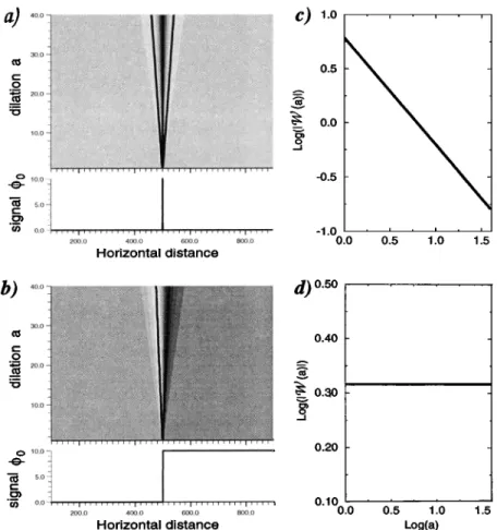
0.40 0.30 0.20 0.10 0.0 0.5 1.0 1.5 Log(a)Figure 2.
Wavelet transforms
of a (a) Dirac distribution
with regularity
c• -- -1 and a (b)
Heaviside distribution with c• = 0. The grey maps (dark grey levels for negative values and
light grey levels for positive values) represent the amplitude (in arbitrary units) of the wavelet
transform of the signals shown just below. The analyzing wavelet is shown in Figure lb. Observe
the typical cone-like structure of the wavelet transforms pointing toward the homogeneity center
of the analyzed functions. This cone-like geometry can easily be tracked with the ridges (black
solid lines) of the wavelet transforms. (c,d) The modulus of the wavelet transform is taken along
the ridge and plotted as a function of the dilation a. In this log-log diagram, the modulus of the wavelet transform varies linearly with a slope equal to the regularity c• of the analyzed
homogeneous function.
where the Poisson kernel is given by
p
(x)-
c,+z
(1
+ Ixl=)
Also, observe that the harmonic continuation may be
written under the form of a wavelet transform and that
the Poisson kernel verifies the semigroup property,
7)zp * 7)z,p- 7)z+z'p, (13)
which will play a fundamental role in the remainder of this paper.
We shall now specialize our study to the particu-
lar class of potential fields produced by homogeneous
sources. So, consider now the Poisson equation
V•½5
(q) -- -er (q) q e I• "+'•,
where the source term rr (q) is assumed to be a homo-
geneous
distribution
of degree
c• (for example,
a dipole)
with respect to the point (0, zo _< 0) and whose support
is a subset of the lower half-space IR" x IR-. We have
½
-
zo],
and the potential field corresponding to such a homo-
geneous source also is homogeneous of degree c• + 2,
i.e.,
½ 5, z
(16)or, introducing the measured field d0 (as),
/).x½o
(x) - A-"-ø•-2½
Ix, (1 - A) Zo.],
(17)where the dilation operator acts on the first n variables
(i.e., x) only. This last expression shows that for ho-
mogeneous potential fields the dilation operator essen-
tially acts like a continuation operator. Indeed, compar-
ing (10) and (17), we obtain the following equivalence:
5006 MOREAU ET AL.' WAVELET ANALYSIS OF POTENTIAL FIELDS 2.3. Wavelet Analysis of Homogeneous
Potential Fields
We now use the properties recalled in sections 2.1 and
2.2 to derive the main result of this paper. We begin
with the covariance of the wavelet transform (equation
(3)) with respect
to dilation and the homogeneity
of the
field •b (equation
(17)) to obtain the following'
w [•, •0] (•, •) - •"w [•, v•0] (•, •)
= ,X-"-2W [#, • (x, (1 - A) z•)] (Ab,
Aa)(19)
Now the harmonic continuation (equation (10)) gives
d [x, (1 - A) z•] - [V(•_•)•.p, d0]
(x),
(20)
which, inserted into (19), reads
w Is, •0] (•, •) - •-•-• [(v(•_•)•p, v•) g, •0] (•).
(21)
Here we have written the wavelet transform as a convo-
lution product as in (1).
2.4. Wavelets Based on the Poisson Semigroup
We now introduce a new class of wavelets possessing
remarkable properties under the Poisson semigroup and
which allows a nice simplification of (21) into a form
very similar to (5) obtained
for homogeneous
functions.
The wavelets belonging to this class are such that the
harmonic continuation acts like a dilation as in (18),
(vp
, ) -
)
where
both the scaling
factor
c and the dilation
a"
depend
on a, a', and g only. Provided
the analyzing
wavelet g satisfies (22), (21) simplifies into
w[g, 40] (•, a) -
•-•-• [cV•,,g, 40] (•)
which furnishes a relation between the voices of the
wavelet transform of the homogeneous field.
A remaining task is to obtain explicit expressions for c
and a" in terms
of a, A, and z•. It can
be shown
[Moreau
et al., 1997]
that a whole
class
of wavelet
satisfying
(22)
can be constructed by applying a linear operator i to
the Poisson kernel p, i.e.,
g - Cp. (•4)
We have shown that a su•cient condition to satisfy (22)
is that i be a Fourier multiplier homogeneous of degree
7, i.e., such that
A A A
c -•(•),
) •(•)•(•)
•(•) - • (•),
(•)
where fi(u) stands
for the Fourier transform
of p(x).
Several wavelets obtained with the operator œ acting
as O/Ox, 02/Ox
•, and Oa/Ox
a are shown
in Figure 1.
Their expressions are
#(x) - -(2/rr) x(lq-x•)
-2
(26)
#(x) - -(2/•r)(1-3x 2) (lq-x•)
-a, (27)
#(x) - (24/•r)(1-x
•) (l+x2) -4,
(28)
respectively. For this class of wavelets, (23) can be re-
duced to the following simple form' w[a, o0] (,, •):
,
- •a 29)
a -- za a q- za •
It can be observed that this expression is very similar to
(5) except that the zo term is present in both the scal-
ing and dilation factors on the right-hand side. This results in a fundamental difference in the geometrical translation of this equation since, contrary to the case
of homogeneous functions for which the cone-like pat-
tern converges on the hyperplane a = 0 (Figure 2), the
cone-like pattern implicit in (29) converges below this
hyperplane at the negative dilation a = zo (see Figure
3 and the discussion in section 2.5). Indeed, up to the
following scaling and change of coordinates,
w[g, 40] (•, •)
)
w[g, 40] (•, •) (•0)
a ) a- z•, (•1)
(29) can be rewritten under a form identical to (6)'
w Is, O0]
(,, a') -
va,/•w Is, O0]
(,, a).
(•)
In a way very similar to that which can be done for ho-
mogeneous functions, the wavelet transform then allows
for a straightforward determination of the regularity c• of the source causing the analyzed potential field. 2.5. Synthetic Example
This example illustrates the application of (32) to po-
tential fields created by isolated homogeneous sources.
We work in a two-dimensional physical space corre-
sponding to n - 1. The first example is shown in Figure
3a and corresponds to the potential of a vertical dipole
located at x = 300 and zo = -20. This dipolar source can be written as a (x, z) = (O/Oz)5 (x - 300, z + 20) and has a homogeneity c• = -3. The example shown in
Figure 3b corresponds to a quadrupolar source with a
regularity c• = -4. The wavelet transforms of the fields
produced by these sources have been computed with
the wavelet shown in Figure i (7 = 1) and have a cone-
like structure very similar to the one obtained when
analyzing homogeneous functions. However, as already
said, the ridges now converge toward the homogeneity
center of the source, i.e., below the line a = 0. We then observe that the wavelet transform of potential
MOREAU ET AL.: WAVELET ANALYSIS OF POTENTIAL FIELDS 5007 -[---•-" •'"'"'"'"'"'"'"••>••••••••••..,"...:•'•i:!'• -::'&-i--';i', ..?: 25 o-[ •-"•-"•'<•'"'"'""' '"'•••'•'•'•>••••••':"',<•:-'"•::•:::::: •i•.:•:...-• •::•' •'••••••••
L
0. •', , , I , , , , I , , , , I , , • , I • • • • I • , , • I 100.0 200.0 3•.0 400.0 5•.0 600.0 Horizontal distance 0.0 10.0 20.0 30.0 40.0 50.0 Dilation • -3.3 ._.1 -3.8 1.2 1.4 1.8 1.8 Log(dilation + z) 0.0' -25.0' , [ i , i , , , , i , , , , , , , i , -1 , i i i , ] , i 100.0 200.0 300.0 400.0 500.0 600.0 Horizontal distance)
...
_.0001 ß •:: .o0002 _.0003 0.0 10.0 20.0 30.0 40.0 50.0f) -3.8 Dilation
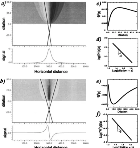
-5.8 1.2 ... 1.4 1.8 1.8 Log(dilation + z)Figure 3. Wavelet transforms of potential fields caused by a (a) vertical dipole and by a (b)
quadrupole. The analyzing wavelet is the one shown in Figure la. As for pure singularities
(see Figure 2), these wavelet transforms also display a cone-like pattern, but it points toward
the location of the homogeneity center at a negative dilation corresponding to the depth of the
causative source. (c,e) When plotted in a log-log diagram, the amplitude of the wavelet transform
along the ridges does not vary linearly. (d,f) Instead, both a change of coordinates and a scaling
are necessary to recover the linear variation with a slope equal to the homogeneity of the source
term.
markable geometrical property which allows for an easy location, both horizontal and vertical, of the causative
sources. The amplitude of the wavelet transforms taken
along the ridge does not vary linearly as observed for the
ridges of the wavelet transforms of homogeneous func-
tions; instead, a scaling (equation (30)) and a change
of coordinates (equation (31)) are necessary to recover
a linear law with a slope fi: -7 + • + 2.
3. Practical Issues
3.1. Analyzing Noisy Da•a
We now address the influence of noise in the detection
procedure explained above. Suppose that the data d (x)
are such that
(x) - (x) +. (x), (aa)
where y (x) represents the noise present in the data to
be analyzed. Of course,
142
[g, d] (b, a) - 142
[g, •b0]
(b, a) + 142
[g, ,] (b, a), (34)
which shows that the wavelet transform of the data
is the sum of a deterministic part 142 [g, •b0] (b, a) with
a stochastic process 142 [g, y] (b, a) whose influence de-
pends on the statistical nature of the noise. For in-
stance, if • (x) is Gaussian white noise with zero mean
2 the linearity of the wavelet transform and variance •r•,
ensures that 142 [g, •] (b, a) is also Gaussian noise with a
variance
rr•v[a,v
] (a)
(35)
where
Eg - f_+• g2
(()d( is the
energy
of the analyz-
ing wavelet. Equation (35) shows that the variance of
]4; [/7, u] (b, a), which is also the variance of the wavelet
transform of the data, varies like a -1 Thus the fluc-
$008 MOREAU ET AL.' WAVELET ANALYSIS OF POTENTIAL FIELDS wavelet transform at small dilations will be more cor-
rupted by the noise than it is at large dilations. Asymp- totically, we expect that
w is, 4
a >>
W iS,
a),
and
14' [g, d] (b, a << ac) •- W[g, u] (b, a) ,
(37)
where ac is a corner dilation corresponding to a signal-
to-noise ratio of the order of 1. This asymptotic be- havior can be checked in Figure 4, which represents the wavelet transforms of the same potential fields as those in Figure 3 but corrupted by a Gaussian white
noise. We observe that for small dilations the ampli-
tude of the wavelet transform taken along the ridges strongly departs from the linear variation related to the
deterministic part of the wavelet transform (after apply-
ing the scaling and the translation). This linear vari- ation is preserved at sufficiently large dilations where
the stochastic part of the wavelet transform becomes
negligible. As can be checked in Figure 4, the corner dilation a• is well defined, and the slope of the ridge is
stable for a > a•. The cone-like pattern is distorted by the stochastic part of the wavelet transform, but as can
be observed, this distortion is minimized for the lines
of extrerna where the signal-to-noise ratio is maximum.
This is why these lines remain accurately straight and intersect near the right depth zo as long as only the
dilations a > a• are considered. This example shows that the wavelet analysis can be locally adapted with
respect to the signal-to-noise ratio depending on the
relative amplitude of the analyzed anomalies compared with the noise amplitude. This constitutes an advan-
tage not shared by the Euler deconvolution method.
3.2. Fields Produced by Extended Sources The analyzed potential fields are always caused by distributed sources which cannot be represented by a
single homogeneous source. In such a situation the mea-
sured field ½0 can be written as a convolution product,
½0
(x) -
dz [s (., z), (7 (., z)] (x),
(38)
where s (x, z) is the source term and (7 (x, z) is a suit-
able Green function. The wavelet transform of the field ½0 reads
W[g, d0] (b, a) - rag * s (., z), G (., z) dz (b)
= 7)aœp, s (-, z), G (-, z)dz (b)
= V•L, V•p, s (-, z), G (., z)dz (b)(39)
where the last line h• been obtained by writing the action of the Fourier multiplier • as the convolution
product L.. Rearranging the terms and introducing
the transformed source distribution
(x,
(.,
(x),
(40)
we obtain W [g, do] (a, a) = vp, a(-,4da
•sœ
(.,
z),
G
(-,
z)dz]
(b).
(41)
1 2•.,,,,,,.,,,....•...:•...•....,.•:••.,..,•...,....•`...•...,.:•,,.,.•`:•,...,,....•,;.,.••.•.:!I•::.::.
...
... '•;•"
-25.0 0.1 -• 0.0 100.0 200.0 300.0 400.0 500.0 600.0 -2.0 -4.0 1.2line
1
-2.22•
, • , , , • . 1.4 1.6 1.8 Log(dilation+z) -4.0 ' • , ' • , 1.2 1.4 11.6 1.8Horizontal Distance Log(dilation+z)
Figure 4. (left) Wavelet transform of the example signal shown in Figure 3a but polluted by
Gaussian white noise. Many lines of extrema have appeared owing to this noise, but the two
lines (labeled I and 2) observed
in Figure 3 and corresponding
to the deterministic
part of the
wavelet transform remain unaltered except for small dilations, and they converge toward the right
location of the source. (right) When properly scaled, the ridges are accurately straight beyond a
MOREAU ET AL.' WAVELET ANALYSIS OF POTENTIAL FIELDS 5009
The source sL (x, z) produces the transformed potential
field
•0,L (x) -
dz [sr (-, z), G (., z)] (x),
(42)
and we finally obtain the following expression for the
wavelet transform of the measured field •b0:
142 [#, q•0] (b, a) = a • [•ap * •0,r] (b). (43)
Comparing this equation with (10), we observe that the
wavelet transform of •0 is the harmonic continuation
•r (x, a) of the field •0,r (x) caused by the transformed
3.3. Choosing the Analyzing Wavelet
We now address the question of the choice of the an-
alyzing wavelet g. In the case of a distributed source s (x, z), the analyzing wavelet plays an important role
since it controls the properties of the transformed source
distribution sr (x, z). In practice, we want the analyz- ing wavelet to produce a transformed source composed
of scattered homogeneous sources in order to locally
apply the theory developed in section 2. However, re- call that the operator • which defines the analyzing wavelet acts through a convolution over the x variable only (see equation (40)) and that the vertical dimen-
sion z is not directly accessible. From the point of view of inverse problem theory, this translates into the
fact that all sources s (z) independent of the horizon-
tal variable x belong to the null space of the wavelet
transform in the sense that such sources produce con-
stant potential fields with a vanishing wavelet trans- form. This implies that the wavelet transform only en-
ables the detection of horizontal variations in the source
s (x, z). For the frequently
encountered
situation
where
the source is smooth almost everywhere and possesses
sharp variations occupying a sparse subset of • x •-
(e.g., juxtaposition of homogeneous blocks), the trans-
formed source s• (x, z) takes large values only in the neighborhood of the horizontal sharp variations.
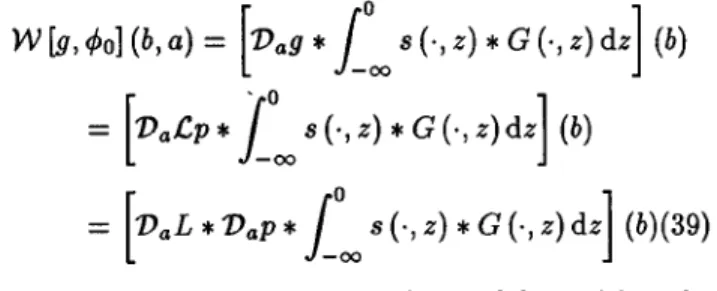
Figure 5 shows the example of a prismatic source with a constant vertical magnetization inside the prism and no magnetization elsewhere. The left edge of the prism
is vertical, and the right one is inclined rightward (45ø).
The depth to top equals 20, and the depth to bottom equals 80 units of length. The wavelet transform com- puted with g (x)= (d/dx)p(x) (7 = 1) (Figure 5, top) takes large values above the lateral edges of the prism and small ones above the horizontal edges. The trans- formed source s• (x, z) = (d/dx) s (x, z) is physically made of two lines of dipolaf sources located on the lat- eral edges of the prism. Since there is only one line of maxima above each edge, the depth of the source can- not be determined by looking for the intersection of the lines of maxima as in the preceding examples. Instead, the depth can only be determined by looking for the values of z• at which the ridges become linear under
12 I i i , -45 7 =3, d3/dx3 1 2 3 4 S 6
,000
ß .. -2• -33 i [ i , I i i i i I [ [ i i I i i i i I , ] i , I 1000.0 2000.0 3000.0 4000.0 5000.0 Horizontal DistanceFigure 5. Wavelet transforms of the potential field
produced by a prismatic body with a vertical left edge
and an inclined (45 ø
) right one. The depth to top of
the prism equals 20 units length and the depth to bot- tom equals 80 units length. The prism has a constant
vertical magnetization. These wavelet transforms have
been obtained with the three wavelets shown in Figure
i and corresponding
to different
operators
/2 (see text
for a detailed discussion).
the scaling defined by (30) and (31). Since 7 is known,
the only variable parameter is zo, which, in practice, is determined by spanning an a priori depth interval and by quantifying the linear character of the transformed
experimental ridge by fitting (in the least squares sense
in the present study) a polynomial of degree 1. This is shown in Figure 6 (middle) where the L2 misfit curves
possess a single minimum. The slope fi of the fitted
lines is also given in Figure 6 (top). We observe that
fi _• -1 so that c• _• -2, which is compatible with the
fact that the transformed source is a line of dipoles, i.e.,
a finite integral of dipoles along the edges of the prism. The best-fitting depths are 37 and 47 units of length for
the left and right edge, respectively. The ridges rescaled
according to these values are shown in Figure 6 (bot-
tom) and appear accurately linear. The depth obtained
5010 MOREAU ET AL.' WAVELET ANALYSIS OF POTENTIAL FIELDS •7 20 40 60 80 100
.... (1)
'
best
slop••
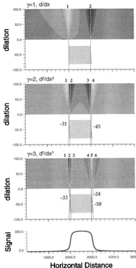
20 40 60 80 100 de•[h •7 20 40 60 80 100 _ _ _ 20 40 60 80 100 deoth 0.8 • 0.4 "• O0 -0 2 14 (•) 1 •6 1.8 2 0 log(a+37) 0.3 (2) -0 2 , I , I , 2.2 1.4 1.6 1.8 2.0 2.2 log(a+4?)Figure 6. Results of the inversion of the ridges extracted from the wavelet transform displayed in the top of Figure 5 and obtained with the L - d/dx operator producing the 7 = i wavelet
shown in Figure la. (top) Corresponding slope/• of the least squares line is adjusted for each
value of z•,. (middle) Misfit between the least squares line and the rescaled ridge is shown as a
function of the parameter z•,. (bottom) Ridges were rescaled with the best z•, obtained by the
least squares analysis.
edge, while the depth derived for the inclined edge falls near the barycenter of the edge.
The wavelet transform shown in Figure 5 (middle)
corresponds
to the analyzing
wavelet
g (x)= (d2/dx
')
p (x) (7 = 2), and the transformed source corresponds
to two lines of quadrupolar sources located on the lat- eral edges of the prism. Two lines of extrema exist above each edge, and as for the preceding example,
the misfit curves possess a single minimum. The depths
found for the left vertical edge are very similar, as and 30 for lines 1 and 2, respectively, while those for the right inclined edge are quite different: 32 for line 3 lo- cated near the shallow end of the edge and 64 for line 4 located toward the deep end of the edge. The depth
obtained from the intersection of the ridges (see Figure
5) equals 31 for the left edge and is consistent with the
results obtained from the least squares analysis just dis-
cussed. The depth obtained for the right edge roughly
falls just between the two depths obtained by analyzing
the two ridges independently. The ridges rescaled ac-
cording to the optimal depths are found to be accurately
linear as in the preceeding example. The slopes for lines
1, 2, and 3 fall near -1.75, and the slope for line 4 is larger (-2.14). These values fall near the theoretical
value -2 corresponding to a pure dipolaf source, and
they are compatible with the fact that the transformed sources are finite integrals of quadrupolar sources.
The wavelet transform shown in Figure 5 (bottom)
corresponds
to the analyzing
wavelet
# (x) - da/dxap
(x)
(7- 3). The transformed source corresponds to two
lines of octupolar sources located on the lateral edges of the prism, and now three lines of extrema converge above each lateral edge of the prism (Figure 5). Lines 1, 2, and 3 form a symmetrical pattern above the left
edge of the prism and converge toward a common point
located at a depth of 33 units of length. The three lines
associated with the right edge are not symmetrical and
do not converge toward a common point. Instead, lines
4 and 5 converge at a depth of 24 units while the right-
most line cuts the two companion lines at greater depths
(50 and 75). The depths obtained for each of the three
ridges located on the left edge are quite similar: 21.5, 23.9, and 21.5 for lines 1, 2, and 3, respectively. The
best fi are also very similar: -2.29,-2.50, and -2.29
for lines 1, 2, and 3. As in the former two examples, the rescaled ridges are linear. The depths obtained by analyzing the three ridges located above the right edge
are consistent with the one derived from the intersec-
tion of the lines of extrema (see Figure 5). Lines 4 and 5 have corresponding depths equal to 17.9 and 21.5,
respectively, and they fall near the shallow end of the
right edge, while the depth for line 6 equals 75.2 and falls near the deep end of the edge.
MOREAU ET AL.- WAVELET ANALYSIS OF POTENTIAL FIELDS 5011
is not directly applicable to extended sources, the three
examples presented above show that the wavelet trans- form yet enables us to locate, both horizontally and ver-
tically, the sharp edges of extended sources. The depths
obtained with the ridges fall within the depth range of the detected edges, and for the vertical edge these depths correspond to the upper part of the source. Fur-
thermore,•
the larger
7, the shallower
the depths.
This
can be explained by the fact that the transformed source is made of multipoles of larger order when 7 is larger
and that the resulting
potential
field is less
controlled
by the deep parts of the source. For the inclined edge, the depth obtained with the 7 - i wavelet falls near the barycenter of the edge, but for larger 7 the situa- tion becomes more complicated since the higher order of derivation eventually allows the separation of the ex- tremities of the edge as is particularly clear for the 7 = 3 example. However, it must be recalled that the 7 = 3 analyzing wavelet amplifies the noise present in the data and that the small dilations are more corrupted than those for the 7 - i case.
4. Field Example
We now briefly discuss an application of the wavelet transform to a near-surface magnetic survey where the two-dimensional approximation is valid. This enables a much easier representation of the results than that in a full three-dimensional geometry. In this example the data were acquired in a small area over a steel pipe carrying hot water across our university campus. Since the location of the pipe is well known, this example provides a tight control of the method. The measure- ments were made with a magnetometer operating at a sampling interval of 0.25 m. The total duration of
the survey was less than a quarter of an hour so that
no diurnal correction was needed. The intensity of the
magnetic field recorded along tracks perpendicular to
the pipes is shown in Figure 7 (bottom).
The wavelet transform of the data is also shown in
Figure 7 (top) and was computed with the analyzing
wavelet shown in Figure la. The analysis of the ridges
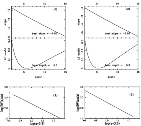
associated with these two lines (Figure 8) gives a depth
of 5.8 and 5.3 unit lengths, i.e., 1.5 and 1.3 m. These
values fully agree with the value (1.6 m) given on the
campus map. The best slopes fi equal -2.65 and -2.85
and give source homogeneities a of the same value be-
cause one must add one more derivative to 7 since we analyze a magnetic field instead of a potential. The
a values obtained fall very near the theoretical value
(-3.0) corresponding to a pure dipolar source. The
ridges rescaled according to the best depths found are
shown in Figure 8 (bottom). One can observe that the
rescaled ridges are accurately linear on the whole dila-
tion interval and that no noise effect is apparent in the
small dilation part (for comparison, refer to Figure 4
and to section 3.1 concerning the effects of noise).
5. Conclusion
The method presented in this study belongs to the
class of the processing methods which transfer the in-
formation content of the data into an auxiliary space. Here the target space is the continuous wavelet trans- form domain where the local homogeneity of the ana- lyzed field can be easily obtained. We have shown that the lines of extrema of the wavelet transform provide a sufficient subset containing the relevant information necessary to recover the main parameter of the homo-
geneous causative sources (depth, horizontal location,
5xlO 4 4.8x10 4
wavelet transform
Time
Figure 7. (top) Wavelet transform and (bottom) magnetic profile displayed for the analyzing
5012 MOREAU ET AL.' WAVELET ANALYSIS OF POTENTIAL FIELDS 5 10 15 ? ? I , , I , , , , I , , , , be 5 10 15 deoth 10 15
'•
' (z)
best
slop•
, , , I , , , _ 10 15 deuth 3.0 1.5 0.8•
(!)
• , , , , 0'.9 1.0 1.1 1.2 log(a+5.8) •.0 [ i ' i ' ! i (2) :2.5 2.0 1.5 I , I , I , 0.8 0,9 1.0 1.1 1.2 log(a+5,3)Figure 8.
(top and middle)
Results
(see
caption
of Figure
6 for details)
of the inversion
of
the ridges extracted from the wavelet transform displayed in Figure 7 and obtained with the
L - d/dx operator
(analyzing
wavelet
in Figure la). (bottom)
Observe
that the rescaled
ridges
are linear on the whole dilation interval and that no noise effect is visible at small dilations.
strength, and degree of homogeneity). The comprehen-
sive theory available for homogeneous sources is use-
ful to understand the wavelet transforms of fields pro-
duced by extended sources, for which the homogeneity hypothesis is not valid. For such sources the choice of the analyzing wavelet is important since it allows for a segmentation of the initial extended source into a small
number of quasi-homogeneous sources. In the case of
extended sources the wavelet transform allows a local
analysis of the measured field. The synthetic examples
show that the noise can efficiently be taken into account
and in a nonstationary way. The examples concerning an extended source show that the wavelet analysis al-
lows a local study of the structural elements (edge, cor-
ner, etc.) of the whole source. The application of the
method to a simple field example further demonstrates the easy use of this technique, which can easily be im- plemented on portable computers and operated by field practitioners.
Acknowledgments. This paper benefited from com-
ments made by Associate Editor Patrick Taylor, Richard Hansen, and an anonymous reviewer. We also had numer- ous discussions with our colleagues Alex Grossmann, Jean Morlet, and Pascal Sailhac. The present study has been granted by the Centre National de la Recherche Scientifique (CNRS-INSU) via ATP Tomographie.
References
Alexandrescu, M., D. Gibert, G. Hulot, J.-L. Le MouE1, and G. Saracco, Detection of geomagnetic jerks using wavelet analysis, J. Geophys. Res., 100, 12557-12572, 1995. Alexandrescu, M., D. Gibert, G. Hulot, J.-L. Le MouE1, and
G. Saracco, Worldwide wavelet analysis of geomagnetic jerks, J. Geophys. Res., 101, 21975-21994, 1996.
Blakely, R.J., Potential Theory in Gravity and Magnetic Ap- plications, Cambridge Univ. Press, New York, 1995. Gibert, D., and A. GaldEano, A computer program to per-
form transformations of gravimetric and aeromagnetic surveys, Cornput. Geosci., 11, 553-588, 1985.
Goupillaud, P., A. Grossmann, and J. Morlet, Cycle-octave and related transforms in seismic signal analysis, Geoex- ploration, 23, 85-102, 1984.
Green, A.G., Magnetic profile analysis, Geophys. J. R. As- tron. Soc., $0, 393-403, 1972.
Grossmann, A., M. Holschneider, R. Kronland-Martinet, and J. Morlet, Detection of abrupt changes in sound sig- nals with the help of wavelet transforms, in Advances in Electronics and Electron Physics, vol. 19, pp. 289-306, Academic, San Diego, Calif., 1987.
Holschneider, M., On the wavelet transformation of fractal objects, J. Star. Phys., 50, 953-993, 1988.
Holschneider, M., Wavelets: An Analysis Tool, Clarendon, Oxford, England, 1995.
Hornby, P., F. Boschetti, and F.G. Horowitz, Analysis of potential field data in the wavelet domain, Geophys. J. Int., in press, 1999.
MOREAU ET AL.' WAVELET ANALYSIS OF POTENTIAL FIELDS $013
Wavelet analysis of potential fields, Inverse Probl., 13, 165-178, 1997.
Parker, R.L., Geophysical Inverse Theory, Princeton Univ. Press, Princeton, N.J., 1994.
Sowerbutts, W.T.C., Magnetic mapping of the Butterton Dyke: An example of detailed geophysical surveying, J.
Geol. Soc. London, 144, 29-33, 1987.
Spector, A., and F.S. Grant, Statistical models for interpret- ing aeromagnetic data, Geophysics, 35, 293-302, 1970. Thompson, D.T., EULDPH: A new technique for making
computer-assisted depth estimates from magnetic data,
Geophysics, 4{ 7, 31-37, 1982.
D. Gibert, F. Moreau, and G. Saracco, G•osciences
Rennes, Universit• de Rennes 1, B&t. 15 Cam-
pus de Beaulieu, 35042 Rennes cedex, France. (e-
mail: gibert @univ-rennes 1.fr; moreau@univ-rennes 1.fr;
ginet @uni v-rennes 1 .fr)
M. Holschneider, Centre de Physique Thdorique, CNRS
Luminy, Case 907, 13288 Marseille, France. (e-mail:
hols @ cpt. univ- mrs. fr)
(Received July 21, 1998; revised October 19, 1998; accepted November 30, 1998.)