HAL Id: hal-00808620
https://hal.archives-ouvertes.fr/hal-00808620
Submitted on 5 Apr 2013
HAL is a multi-disciplinary open access
archive for the deposit and dissemination of
sci-entific research documents, whether they are
pub-lished or not. The documents may come from
teaching and research institutions in France or
abroad, or from public or private research centers.
L’archive ouverte pluridisciplinaire HAL, est
destinée au dépôt et à la diffusion de documents
scientifiques de niveau recherche, publiés ou non,
émanant des établissements d’enseignement et de
recherche français ou étrangers, des laboratoires
publics ou privés.
Sachs Wolfe Effect
François-Xavier Dupé, Anais Rassat, Jean-Luc Starck, Jalal M. Fadili
To cite this version:
François-Xavier Dupé, Anais Rassat, Jean-Luc Starck, Jalal M. Fadili. An Optimal Approach for
Measuring the Integrated Sachs Wolfe Effect. Astronomy and Astrophysics - A&A, EDP Sciences,
2011, 534 (A51), 16 p. �10.1051/0004-6361/201015893�. �hal-00808620�
March 29, 2011
An Optimal Approach
for Measuring
the Integrated Sachs Wolfe Effect
F.-X. Dup´e
1 !, A. Rassat
1 !!, J.-L. Starck
1, and M. J. Fadili
21 Laboratoire AIM, UMR CEA-CNRS-Paris 7, Irfu, SAp/SEDI, Service d’Astrophysique, CEA Saclay, F-91191
GIF-SUR-YVETTE CEDEX, France.
2 GREYC UMR CNRS 6072, Universit´e de Caen Basse-Normandie/ENSICAEN, 6 bdv Mar´echal Juin, 14050 Caen,
France.
Preprint online version: March 29, 2011
ABSTRACT
Context. One of the main challenges of modern cosmology is to understand the nature of the mysterious dark
en-ergy which causes the cosmic acceleration. The Integrated Sachs-Wolfe (ISW) effect is sensitive to dark enen-ergy and if detected in a universe where modified gravity and curvature are excluded, presents an independent signature of dark energy. The ISW effect occurs on large scales, where cosmic variance is high and where there are large amounts of missing data in the CMB and large scale structure maps due to Galactic confusion. Moreover, existing methods in the literature often make strong assumptions about the statistics of the underlying fields or estimators. Together these effects can severely limit signal extraction.
Aims. We want to define an optimal statistical method for detecting the ISW effect, which can handle large areas of
missing data and minimise the number of underlying assumptions made about the data and estimators.
Methods. We first review current detections (and non-detections) of the ISW effect, comparing statistical subtleties
between existing methods, and identifying several limitations. We propose a novel method to detect and measure the ISW signal. This method assumes only that the primordial CMB field is Gaussian. It is based on a sparse inpainting method to reconstruct missing data and uses a bootstrap technique to avoid assumptions about the statistics of the estimator. It is a complete method, which uses three complementary statistical methods.
Results. We apply our method to Euclid-like simulations and show we can expect a ∼ 7σ
model-independent detection of the ISW signal with WMAP7-like data, even when considering missing data.
Other tests return ∼ 4.7σ detection levels for a Euclid-like survey. We find detections levels are
inde-pendent from whether the galaxy field is normally or lognormally distributed. We apply our method
to the 2 Micron All Sky Survey (2MASS) and WMAP7 CMB data and find detections in the 1.1− 2.0σ
range, as expected from our simulations. As a by-product, we have also reconstructed the full-sky temperature ISW field due to 2MASS data.
Conclusions. We have presented a novel technique, based on sparse inpainting and bootstrapping, which accurately
detects and reconstructs the ISW effect.
Key words. ISW, inpainting, signal detection, hypothesis test, bootstrap
1. Introduction
The recent abundance of cosmological data in the last few decades (for an example of the most recent results see Komatsu et al. 2009; Percival et al. 2007 a; Schrabback et al. 2010) has provided compelling evidence towards a standard concordance cosmology, in which the Universe is composed of approximately 4% baryons, 26% ‘dark’ matter and 70% ‘dark’ energy. One of the main challenges of mod-ern cosmology is to understand the nature of the mysterious dark energy which drives the observed cosmic acceleration (Albrecht et al. 2006; Peacock et al. 2006) .
The Integrated Sachs-Wolfe (ISW) (Sachs & Wolfe 1967) effect is a secondary anisotropy of the Cosmic Microwave Background (CMB), which arises because of the
variation with time of the cosmic gravitational potential between local observers and the surface of last scattering. The potential can be traced by Large Scale Structure (LSS) surveys (Crittenden & Turok 1996), and the ISW effect is therefore a probe which links the high redshift CMB with the low redshift matter distribution and can be detected by cross-correlating the two.
As a cosmological probe, the ISW effect has less statis-tical power than weak lensing or galaxy clustering (see for e.g., Refregier et al. 2010), but it is directly sensitive to dark energy, curvature or modified gravity (Kamionkowski & Spergel 1994; Kinkhabwala & Kamionkowski 1999; Carroll et al. 2005; Song et al. 2007), such that in uni-verses where modified gravity and curvature are excluded, detection of the ISW signal provides a direct signature of dark energy. In more general universes, the ISW effect can be used to trace alternative models of gravity.
The CMB WMAP survey is already optimal for detect-ing the ISW signal (see Sections 2 and 3), and significance is not expected to increase with the arrival of Planck, un-less the effect of the foreground Galactic mask can be re-duced. The amplitude of the measured ISW signal should however depend strongly on the details of the local tracer of mass. Survey optimisations (Douspis et al. 2008) show that an ideal ISW survey requires the same configuration as surveys which are optimised for weak lensing or galaxy clustering - meaning that an optimal measure of the ISW signal will essentially come ‘for free’ with future planned weak lensing and galaxy clustering surveys (see for e.g. the Euclid survey Refregier et al. 2010). In the best scenario, a 4σ detection is expected (Douspis et al. 2008), and it has been shown that combined with weak lensing, galaxy correlation and other probes such as clusters, the ISW can be useful to break parameter degeneracies (Refregier et al. 2010), making it a promising probe.
Initial attempts to detect the ISW effect with COBE as the CMB tracer were fruitless (Boughn & Crittenden 2002), but since the arrival of WMAP data, tens of positive detections have been made, with the highest significance reported for analyses using a tomographic combination of surveys (see Sections 2 and 3 for a detailed review of de-tections). However, several studies using the same tracer of LSS appear to have contradicting conclusions, some anal-yses do not find correlation where others do, and as sta-tistical methods to analyse the data evolve, the signifi-cance of the ISW signal is sometimes reduced (see for e.g., Afshordi et al. 2004; Rassat et al. 2007; Francis & Peacock 2010b).
In Section 2, we describe the cause of the ISW effect and review current detections. In Section 3, we describe the methodology for detection and measuring the ISW signal, and review a large proportion of reported detections in the literature, as well as their advantages and disadvantages. Having identified the main issues with current methods, we propose a new and complete method in Section 4, which capitalises on the fact that different statistical methods are complementary and uses sparse inpainting to solve the issue of missing data and a bootstrapping technique to measure the estimator’s probability distribution function (PDF). In Section 5, we validate our new method using simulations for 2MASS and Euclid-like surveys. In Section 6, we apply our new method to WMAP 7 and the 2MASS survey. In Section 7, we present our conclusions.
2. The Integrated Sachs-Wolfe Effect
2.1. Origin of the Integrated Sachs-Wolfe EffectGeneral relativity predicts that the wavelength of electro-magnetic radiation is sensitive to gravitational potentials, an effect which is called gravitational redshift. Photons trav-elling from the surface of last scattering will necessarily travel through the gravitational potential of Large Scale Structure (LSS) on their way to the observer; these will be blue-shifted as they enter the potential well and red-shifted as they exit the potential. These shifts will accumu-late along the line of sight of the observer. The total shift in wavelength will translate into a change in the measured temperature-temperature anisotropy of the CMB, and can
be calculated by: ! ∆T T " ISW = −2# η0 ηL Φ!((η 0− η)ˆn, η) dη, (1)
where T is the temperature of the CMB, η is the conformal time, defined by dη = dt
a(t) and η0 and ηL represent the
conformal times today and at the surface of last scattering respectively. The unit vector ˆn is along the line of sight and the gravitational potential Φ(x, η) depends on position and time. The integral depends on the rate of change of the potential Φ! = dΦ/dη.
In a universe with no dark energy or curvature, the cos-mic (linear) gravitational potential does not vary with time, so that such a blue- and red-shift will always cancel out, because Φ!= 0 and there will be no net effect on the wave-length of the photon.
However, in the presence of dark energy or curva-ture (Sachs & Wolfe 1967; Kamionkowski & Spergel 1994; Kinkhabwala & Kamionkowski 1999), the right hand side of Equation 1 will be non-null as the cosmic potential will change with time (see for e.g., Dodelson 2003), resulting in a secondary anisotropy in the CMB temperature field. 2.2. Detection of the ISW signal
The ISW effect leads to a linear scale secondary anisotropy in the temperature field of the CMB, and will thus af-fect the CMB temperature power spectrum at large scales. Due to the primordial anisotropies and cosmic variance on large scales, the ISW signal is difficult to detect directly in the temperature map of the CMB, but Crittenden & Turok (1996) showed it could be detected through cross-correlation of the CMB with a local tracer of mass.
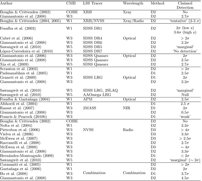
The first attempt to detect the ISW effect (Boughn & Crittenden 2002) involved correlating the Cosmic Microwave Background explorer data (Bennett et al. 1990, COBE) with XRB (Boldt 1987) and NVSS data (Condon et al. 1998). This analysis did not find a significant cor-relation between the local tracers of mass and the CMB. Since the release of data from the Wilkinson Microwave Anisotropy Probe (Spergel et al. 2003, WMAP) over 20 studies (see Table 1) have investigated cross-correlations between the different years of WMAP data and local tracers selected using various wavelengths: X-ray (Boldt 1987, XRB survey); optical (Ag¨ueros et al. 2006; Adelman-McCarthy et al. 2008, SDSS galaxies), (Anderson et al. 2001, SDSS QSOs), (Doroshkevich et al. 2004, SDSS LRGs), (Maddox et al. 1990, APM); near infrared (Jarrett et al. 2000, 2MASS); radio (Condon et al. 1998, NVSS).
The full sky WMAP data have sufficient resolution on large scales that the measure of the ISW signal is cos-mic variance limited. The best LSS probe of the ISW ef-fect should include maximum sky coverage and full redshift coverage of the dark energy dominated era (Douspis et al. 2008). No such survey exists yet, so there is room for im-provement on the ISW detection as larger and larger LSS surveys arise. For this reason, when we review the current ISW detections, we classify them according to their tracer of LSS, and not the CMB map used.
The measure of the ISW signal can be done in vari-ous statistical spaces; we classify detections in Table 1 into three measurement ‘domains’: D1 corresponds to spheri-cal harmonic space; D2 to configuration space and D3 to
Author CMB LSS Tracer Wavelength Method Claimed Detection
Boughn & Crittenden (2002) COBE XRB Xray D2 No
Giannantonio et al. (2008) W3 D2 2.7σ
Boughn & Crittenden (2004, 2005) W1 XRB/NVSS Xray/Radio D2 ‘tentative’ (2-3 σ)
Fosalba et al. (2003) W1 SDSS DR1 D2 2σ (low z)
3.6σ (high z)
Cabr´e et al. (2006) W3 SDSS DR4 Optical D2 > 2σ
Giannantonio et al. (2008) W3 SDSS DR6 D2 2.2σ
Sawangwit et al. (2010) W5 SDSS DR5 D2 ‘marginal’
L´opez-Corredoira et al. (2010) W5 SDSS DR7 D2 ‘No detection’
Giannantonio et al. (2006) W3 SDSS Quasars Optical D2 2σ
Giannantonio et al. (2008) W3 SDSS Quasars D2 2.5σ
Xia et al. (2009) W5 SDSS Quasars D2 2.7σ
Scranton et al. (2003) W1 D2 > 2σ
Padmanabhan et al. (2005) W1 D1 2.5σ
Granett et al. (2009) W3 SDSS LRG Optical D1 2σ
Giannantonio et al. (2008) W3 D2 2.2σ
Sawangwit et al. (2010) W5 SDSS LRG, 2SLAQ D2 ‘marginal’
Sawangwit et al. (2010) W5 AAOmega LRG D2 Null
Fosalba & Gazta˜naga (2004) W1 APM Optical D2 2.5σ
Afshordi et al. (2004) W1 D1 2.5 σ
Rassat et al. (2007) W3 2MASS NIR D1 2σ
Giannantonio et al. (2008) W3 D2 0.5σ
Francis & Peacock (2010b) W3 D1 ‘weak’
Boughn & Crittenden (2002) COBE D2 No
Nolta et al. (2004) W1 D2 2.2σ
Pietrobon et al. (2006) W3 NVSS Radio D3 > 4σ
Vielva et al. (2006) W3 D3 3.3σ McEwen et al. (2007) W3 D3 > 2.5σ Raccanelli et al. (2008) W3 D2 2.7σ McEwen et al. (2008) W3 D3 ∼ 4σ Giannantonio et al. (2008) W3 D2 3.3σ Hern´andez-Monteagudo (2009) W3 D1 < 2σ
Sawangwit et al. (2010) W5 D2 ‘marginal’ (∼ 2σ)
Corasaniti et al. (2005) W1 D2 > 2σ
Gazta˜naga et al. (2006) W1 D2 2σ
Ho et al. (2008) W3 Combination Combination D1 3.7σ
Giannantonio et al. (2008) W3 D2 4.5σ
Table 1. Meta-analysis of ISW detections to date and their reported statistical significance. The ‘Method’ describes the space in which the power spectrum analysis is done (configuration, spherical harmonic, etc . . . ), not the method for measuring the significance level of the detection (this is described in Section 3). D1 corresponds to spherical harmonic space, D2 to configuration space, D3 to wavelet space. The highest detections are made in wavelet space. Regarding the survey used, the highest detections are made using NVSS (though weak and marginal detections using NVSS are also reported) or using combinations of LSS surveys as the matter tracer.
wavelet space. (In Section 3, we review the different meth-ods for quantifying the statistical significance of each mea-surement).
There are only two analyses which use COBE as CMB data (with XRB and NVSS data, Boughn & Crittenden 2002), and both report null detections, which can reason-ably be due to the low angular resolution of COBE even at large scales. The rest are done correlating WMAP data from years 1, 3 and 5 (respectively ‘W1’, ‘W3’ and ‘W5’ in table 1).
Most ISW detections reported in Table 1 are relatively ‘weak’ (< 3σ) and this is expected from theory for a con-cordance cosmology. Higher detections are reported for the NVSS survey (Pietrobon et al. 2006; McEwen et al. 2008; Giannantonio et al. 2008), though weak and marginal
de-tections using NVSS data are also reported (Hern´andez-Monteagudo 2009; Sawangwit et al. 2010). High detections are often made using a wavelet analysis (Pietrobon et al. 2006; McEwen et al. 2008), though a similar study by the same authors using the same data but a different analysis method finds a weaker signal (McEwen et al. 2007). The highest detection is reported using a tomographic combi-nation of all surveys (XRB, SDSS galaxies, SDSS QSOs, 2MASS and NVSS, Giannantonio et al. 2008), as expected given the larger redshift coverage of the analysis.
Several analyses have been revisited to seek confirma-tion of previous detecconfirma-tions. In some cases, results are very similar (Padmanabhan et al. (2005); Granett et al. (2009); Giannantonio et al. (2008), for SDSS LRGs; Giannantonio et al. (2006, 2008) for SDSS Quasars; Afshordi et al. (2004);
Rassat et al. (2007), for 2MASS), but in some cases they are controversially different (for e.g. Pietrobon et al. (2006) and Sawangwit et al. (2010), for NVSS or Afshordi et al. (2004) and Giannantonio et al. (2008), for 2MASS).
We also notice that as certain surveys are revisited, there is a trend for the statistical significance to be re-duced: for e.g., detections from 2MASS decrease from a 2.5σ detection (Afshordi et al. 2004), to 2σ (Rassat et al. 2007), to 0.5σ (Giannantonio et al. 2008) to ‘weak’ (Francis & Peacock 2010b). Detections using SDSS LRGs decrease from 2.5σ (Padmanabhan et al. 2005), to 2 − 2.2σ (Granett et al. 2009; Giannantonio et al. 2008), to ‘marginal’ (Sawangwit et al. 2010). Furthermore, there tends to be a ‘sociological bias’ in the interpretation of the confidence on the signal detection. The first detec-tions interpret a 2 − 3σ detection as ‘tentative’ (Boughn & Crittenden 2004, 2005), while further studies with sim-ilar detection level report ‘independent evidence of dark energy’ (Afshordi et al. 2004; Gazta˜naga et al. 2006).
3. Methodology for Detecting the ISW Effect
In this paper, we are interested in qualifying the differences between different statistical methods which exist in the lit-erature, and comparing them with a new method we present in Section 4. By statistical method, we mean the method which is used to quantify the significance of a signal, not the space in which the signal is measured. Therefore, and with-out loss of generality, the review presented in Section 3.2 summarises methods using spherical harmonics. We com-pare the pros and cons of each method in Section 3.3. We begin by describing how the ISW signal can be measured in spherical harmonics in Section 3.1
3.1. ISW Signal in Spherical Harmonics
In general, any field can be decomposed by a series of functions which form an orthonormal set, as do the spher-ical harmonic functions Y"m(θ, φ). Therefore a projected galaxy overdensity (δg) or temperature anisotropy (δT) field
δX(θ, φ), where X = g, T , can be decomposed into:
δX(θ, φ) = $
",m
aX"mY"m(θ, φ), (2) where aX
"m are the spherical harmonic coefficients of the field. The 2-point galaxy-temperature cross-correlation function can then be written:
CgT(&) = 1 (2& + 1) $ m Re%ag"m(aT "m)∗ & , (3)
where taking the real part of the product ensures that CgT(&) = CT g(&).
The theory for the angular cross-correlation function is given by: CgT(&) = 4πbg # dk∆2(k) k Wg(k)WT(k), (4) where Wg(k) = # drΘ(r)j"(kr)D(z), (5) WT(k) = − 3Ωm,0H02 k2c3 # zL 0 drj"(kr)H(z)D(z)(f − 1), (6) ∆2(k) = 4π (2π)3k 3P (k), (7) Θ(r) = 'rdrr2n(r)2n(r). (8) In these equations, r represents the co-moving distance, zL the redshift at the last scattering surface, k the Fourier mode wavenumber and quantities which depend on the red-shift z have an intrinsic dependence on r: H(z) = H(z(r)). The function f is the linear growth factor given by f =
d ln D(z)
d ln a(z), where D(z) is the linear growth which measures
the growth of structure. The cross-correlation function de-pends on the survey selection function given by n(r), in units of galaxies per unit volume. The quantities Ωm,0and
H0 are the values of the matter density and the Hubble
parameter at z = 0. Units are chosen so that the quantity C(&) is unitless.
In the case where both the temperature and the galaxy fields behave as Gaussian random fields, then the covariance on the ISW signal can be calculated by:
( |CgT|2 ) = 1 fsky(2& + 1) % CgT2 + (Cgg+ Ng) (CT T + NT)&, (9) where CT T is the temperature-temperature power spec-trum, Ng and NT are the noise of the galaxy and temper-ature fields respectively. The galaxy auto-correlation func-tion can be calculated theoretically in linear theory by:
Cgg(&) = 4πb2g #
dk∆2(k)
k [Wg(k)]2, (10)
There are many difficulties in measuring the ISW ef-fect, the first being the intrinsic weakness of the signal. To add to this, an unknown galaxy bias scales linearly with the ISW cross-correlation signal (see Equation 4), which is therefore strongly degenerate with cosmology. Galactic foregrounds in both the CMB and the LSS maps also mask crucial large scale data and can introduce spurious correla-tions. Any method claiming to detect the ISW effect should be as thorough as possible in accounting for missing data, and where possible the reported detection level should be independent of an assumed cosmology.
3.2. Review on Current Tools for ISW Detection
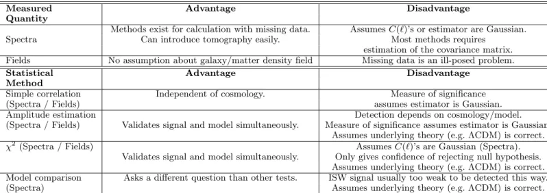
In the literature there are two quantities which can be used to measure and detect the ISW signal, which we review in this section. Without loss of generality, we present these methods in spherical harmonic space. The first method measures the observed cross-correlation spec-tra (‘Specspec-tra’ method: see section 3.2.3), whilst the second directly compares temperature fields (‘Fields’ method: see section 3.2.4). These two approaches differ by the quantity they measure to infer a detection. For each method (fields vs. spectra), it is possible to use different statistical meth-ods to infer detection which we describe below. We review each existing method below and summarise the pros and cons of both of these classes as well as the statistical mod-els in Table 2.
3.2.1. Note on the confidence score
Before reviewing the ISW detection methods, we would like to clarify the definition of confidence
Measured Advantage Disadvantage Quantity
Methods exist for calculation with missing data. Assumes C(")’s or estimator are Gaussian.
Spectra Can introduce tomography easily. Most methods requires
estimation of the covariance matrix.
Fields No assumption about galaxy/matter density field Missing data is an ill-posed problem.
Statistical Advantage Disadvantage
Method
Simple correlation Independent of cosmology. Measure of significance
(Spectra / Fields) assumes estimator is Gaussian.
Amplitude estimation Detection depends on cosmology/model.
(Spectra / Fields) Validates signal and model simultaneously. Measure of significance assumes estimator is Gaussian.
Assumes underlying theory (e.g. ΛCDM) is correct.
χ2 (Spectra / Fields) Assumes C(")’s are Gaussian (Spectra).
Validates signal and model simultaneously. Only gives confidence of rejecting null hypothesis.
Assumes underlying theory (e.g. ΛCDM) is correct.
Model comparison Asks a different question than other tests. ISW signal usually too weak to be detected this way.
(Spectra) Assumes underlying theory (e.g. ΛCDM) is correct.
Table 2. TOP: Review of advantages and disadvantages of measuring spectra vs. fields in order to infer an ISW detection. BOTTOM: Review of statistical methods existing in the literature and their respective advantages and disadvantages.
scores from a statistical point of view. The confi-dence of a null hypothesis test can be interpreted as the distance from the data to the null hypothe-sis (commonly named H0). For example, let ρ be a
variable of interest (e.g. correlation coefficient, am-plitude). The confidence score σ for the hypothesis test H0 (i.e., ρ = 0) against H1 (i.e., ρ #= 0) is directly
computed using the formula τ = ρ/σ(ρ), where σ(ρ) is the standart deviation. But this only true when 1) ρ is Gaussian, 2) σ(ρ) is computed independently of the observation and 3) considering a symmet-ric test. Then, this method does not stand for the general case and as the correlation coefficient con-sidered here must be positive, an asymmetric test (one-sided test) would also be more appropriate here.
Remember that a confidence score is directly linked to the deviation from the H0 hypothesis
through the p-value which is a probability, so the σ-score is always positive. Then the p-value p of one hypothesis test is computed using the proba-bility density function (PDF) of the test distribu-tion: p = 1 −'τ
−∞P (x|H0)dx = '+∞
τ P (x|H0)dx (for a classical one-sided test). Remark that in that case, if the H0 is true then ρ ≈ 0 (i.e. in the middle of the
test distribution) and the p-value p will be around 0.5 which correspond to a confidence of 0.67σ. 3.2.2. Note on the application spaces
All the methods that will be described in the next sections can be performed in different domains. While some spaces may be more appropriate than others for a specific task, difficulties may also arise because of the properties of the space. For example: for the ‘spectra’ method in configura-tion space, the two main difficulties are missing data and the estimation of the covariance matrix (see e.g. Hern´andez-Monteagudo 2008). In this case, the covariance matrix can be estimated using Monte Carlo methods (see Cabr´e et al. 2007). In spherical harmonic space, missing data induce mode correlations which can be removed by using an
appro-priate framework for calculation of the C(&)’s (e.g. Hivon et al. 2002). In harmonic space (when missing data is ac-counted for) the covariance matrix is diagonal and thus easily invertible (see Section 3.2.4).
3.2.3. Cross-power spectra comparison
The most popular method consists in using the cross-correlation function (Equation 4, in spherical harmonic space) to measure the presence of the ISW signal, how-ever this approach has recently been challenged by L´opez-Corredoira et al. (2010), because of its high sensitivity to noise and fluctuations due to cosmic variance.
One of the subtleties of the cross-correlation function method is the evaluation of the covariance matrix Ccovar
and its inverse. This matrix can be estimated using the MC1 or MC2 methods of Cabr´e et al. (2007), in which case the test is strongly dependent on the quality of the simula-tions. Secondly, missing data will require extra care when estimating the power spectra, this can be tackled by us-ing MASTER (Monte Carlo Apodized Spherical Transform Estimator) or QML (Quadratic Maximum Likelihood) methods (Hivon et al. 2002; Efstathiou 2004; Munshi et al. 2009).
The spectra measurement can be used with one of four different statistical methods. The advantages and disadvan-tages of each method are summarised below and in Table 2. The first aims to detect a correlation between two signals, i.e. we test if the cross-power spectra is null or not. The second fits a (model-dependent) template to the measured cross-power spectra. The other two methods aim to validate a cosmological model as well as confirm the presence of a signal: the χ2test and the model comparison. We describe
them below:
– Simple correlation detection: The simplest and the most widely used method for detecting a cross-correlation between two fields X and Y (here suppos-ing that Y is correlated with X) (see e.g. Boughn & Crittenden 2002; Afshordi et al. 2004; Pietrobon et al. 2006; Sawangwit et al. 2010) is to measure the
correla-tion coefficient ρ(X, Y ), defined as: ρ(X, Y ) = Cor(X, Y )/Cor(X, X), where, Cor(X, Y ) = 1 Np $ p Re [X∗(p)Y (p)] , (11) with p a position or scale parameter and Npthe number of considered positions or scales. There is a correlation between the two fields if ρ(X, Y ) is not null. The corre-lation coefficient is linked to the cross-power spectra in harmonic space: ρ(g, T ) = * $ " (2& + 1)CgT(&) + / * $ " (2& + 1)Cgg(&) + . (12) Thus the nullity of the coefficient implies the nullity of the cross-power spectra. A z-score can be performed in order to test this nullity,
K0= ρ/σρ , (13)
where the standard error of the correlation value, σρ can be estimated using Monte Carlo simulations under a given cosmology. In the literature, most applications of this method assume that K0 follows a Gaussian
dis-tribution under the null hypothesis (i.e. no correlation), for example Vielva et al. (2006) and Giannantonio et al. (2008), which is not necessarily true.
The distribution of the K0test can be inferred if we
as-sume that both fields X and Y , of the cross-correlation are Gaussian. In this case, the correlation coefficient dis-tribution is the normally distributed but follows a nor-mal product distribution, which is far from Gaussian. In the case where Y is a constant field, the correlation coef-ficient follows a normal distribution and the distribu-tion of the hypothesis test K0will depend on how
the variance of the estimator σρ is computed. If this last value is derived from the observation X, then K0 follows a Student’s t-distribution which
converges to a Gaussian distribution only when ρ is high (by the central limit theorem). Else, if the variance σρ is estimated independently from the data (through Monte-Carlo, for example) or known for a given cosmology, K0 can be assumed
to follow a Gaussian distribution. This means that K0is generally not Gaussian even if the
cor-relation coefficient is Gaussian (see section 4). This method does not include knowledge of the underly-ing ISW signal, nor of the galaxy field, though the error bars can be estimated from Monte Carlo simulations which include cosmological information.
– Amplitude estimation (or template matching): The principle of the amplitude estimation is to measure whether an observed signal corresponds to the signal predicted by a given cosmological model.
The estimator and its variance are given by (e.g. Ho et al. 2008; Giannantonio et al. 2008):
ˆλ = CgTTh∗Ccovar−1 CgTObs CTh∗ gT Ccovar−1 CgTTh , σλˆ= 1 , CTh∗ gT Ccovar−1 CgTTh , (14) where CTh
gT is the theoretical cross-power spectrum,
CObs
gT the estimated (observed) power spectrum and
Ccovar the covariance matrix calculated by Equation 9.
A z-score,
K1= ˆλ/σλˆ , (15)
is usually applied to test if the amplitude is null or not. – Goodness of fit, χ2 test:
The goodness of fit or χ2 test is given by (e.g. Afshordi
et al. 2004; Rassat et al. 2007):
K2= (CgTTh− CgTObs)∗Ccovar−1 (CgTTh− CgTObs) , (16) where K2 follows a χ2 distribution with number of
de-grees of freedom (d.o.f ) depending on the input data. This tests the correspondance of the data with a given cosmological model, but does not infer if the tested model is in fact the best. Equation 16 also assumes that the C(&)!s are Gaussian variables. The value of χ2gives
a idea on the probability of rejecting the model, but can-not be compared directly with the K2value for the null
hypothesis without careful statistics (see next method on model comparison).
– Model comparison:
The model comparison method is based on the gener-alised likelihood ratio test and asks the question: ‘Do the data prefer a given fiducial cosmological model over the null hypothesis ?’. This question is important because it could be possible to use the previous χ2test to detect
an ISW signal - yet the data could still also be compat-ible with a null hypothesis (see for e.g., Afshordi et al. 2004; Rassat et al. 2007; Francis & Peacock 2010b). In this case it is important to perform a model compari-son to find which model is preferred by the data. Two hypotheses are built:
– H0: “there is no ISW signal”, i.e. the cross-power
spectra is null;
– H1: “there is an ISW signal compatible with a fidu-cial cosmology”, i.e. the cross-power spectra is close to an expected one.
One should then estimate:
K3= ∆χ2= (CgTObs)∗Ccovar−1 (CgTObs)− (CTh
gT − CgTObs)∗Ccovar−1 (CgTTh− CgTObs) ,
(17) where K3converges asymptotically to a χ2distribution.
If the value is higher than a threshold (chosen for a re-quired confidence level), the H0 hypothesis is rejected.
However, such method is difficult to use directly because of the small sample bias, K3 is not likely to follow a χ2
statistic. In the case of the ISW signal, the signal for a ‘standard’ fiducial cosmology (e.g., WMAP 7 cosmol-ogy) is so weak that it usually returns a lack of detection for current surveys - this may not be the case for future or tomographic surveys. Notice that this model compar-ison method can be seen as an improved version of the goodness of fit.
3.2.4. Field to field comparison
Instead of comparing the spectra, one can work directly with the temperature field to measure the presence of the ISW signal. The observable in this case is now the ISW temperature field (δISW), rather than the cross-correlation
power spectra CgT(&). The observed CMB temperature anisotropies δOBS can be described as:
where δISW is the ISW field and λ its amplitude (normally
near 1), δT the primordial CMB temperature field, δother
represents fluctuations due to secondary anisotropies other than the ISW effect and N represents noise. In the context of the ISW effect, which occurs only on large (linear) scales where noise and other secondary anisotropies are negligible, we have:
δOBS% δT + λδISW . (19)
The main difference between the fields and spectra ap-proach is that the fields method requires an estimation of the ISW temperature field (δISW). There are several
meth-ods to calculate δISWfrom a given matter overdensity map.
The most accurate way to reconstruct the ISW sig-nal is to use information from the full 3-dimensiosig-nal matter distribution, which in theory requires over-lapping galaxy and weak lensing maps on large scales. This may be possible in the future with sur-veys like Euclid (Refregier et al. 2010). Assuming a simple bias relation, the matter field can also be es-timated directly from galaxy surveys (see Granett et al. 2009, who did this for small patches on the sky). In the case where only the general redshift dis-tribution of the galaxy survey is known, the ISW field δISWcan be approximated directly from the galaxy
and temperature maps using (see Cabr´e et al. 2007): aISW"m =
CgT(&)
Cgg(&)
g"m, (20)
where g"m are the spherical harmonic coefficients of the galaxy map, and aISW
"m the coefficients of the ISW temper-ature anisotropy map. Another approach is to reconstruct the ISW map using Equation 1 where Φ! is estimated using the Poisson Equation (Francis & Peacock 2010a).
Note that the potential which creates the ISW signal is first order in perturbation theory. However, even in the absence of non-Gaussianities in the primordial inflaton field, the potential φ will evolve with redshift, and can become lognor-mal on quasi-linear scales, where the potential is still decaying: this will produce an ISW tempera-ture signal (which is positively correlated with the density field), which will approach Gaussianity on the largest scales but may contain some traces of non-Gaussianity on smaller scales (see Francis & Peacock 2010a,b). On smaller and non-linear scales, the Rees-Sciama effect will produce secondary tem-perature anisotropies which are negatively corre-lated with the density field (Schaefer et al. 2010; Cai et al. 2010).
As for the spectra approach, there are several statistical methods available to qualify detection:
– Simple correlation detection:
The simple correlation detection method described for the spectra comparison, can in fact also be considered as a field comparison. This is the only method which directly overlaps between both approaches.
– Amplitude estimation (or template matching): Using the Gaussian framework, given an ISW field, the amplitude λ can be estimated with the corre-sponding maximum likelihood estimator (Hern´andez-Monteagudo 2008; Frommert et al. 2008; Granett et al.
2009): ˆλ = δISW∗ CT T−1δOBS δ∗ ISWCT T−1δISW , σλˆ= 1 , δ∗ ISWCT T−1δISW . (21)
A signal is present if ˆλ is non null and a z-score,
K4= ˆλ/σλˆ , (22)
directly yields the confidence level in terms of σ. Equation 21 implicitly assumes that the primordial CMB field δT is a Gaussian random field (we discuss this further in section 4).
– Goodness of fit, χ2 test:
The χ2 goodness of fit with H
1 (see Model
compari-son in 3.2.3) yields:
K5= (δISW− δOBS)∗CT T−1(δISW− δOBS) , (23)
where K5is a χ2variable with number of d.o.f
depend-ing on the input data. In this case, the test only returns the confidence of rejecting the null hypothesis H0. As
in the χ2test for the spectra, precaution must be taken
when comparing χ2values for different models, by using
an appropriate model comparison technique. We intro-duce this in section 4.
3.3. Pros and cons of each method
We have identified two main classes of methods: either using power spectra or fields to measure the ISW signal. For each approach one can choose amongst several statistical tools to measure the significance of a correlation or validate si-multaneously a correlation and a model. The advantages and disadvantages of both approaches are summarised be-low and in the top part of Table 2.
One of the main advantages of using the field approach is that it assumes only that the primordial CMB field comes from a Gaussian random process, which is largely believed to be true. In the other approach, the spectra are assumed to be Gaussian, which is not the case. Several stud-ies (Cole et al. 2001; Kayo et al. 2001; Wild et al. 2005) have also shown that the matter overdensity exhibits a lognor-mal behavior on large scale. The bias introduced has been shown to be small (Bernardeau et al. 2002; Hamimeche & Lewis 2008), however this approach is still theoretically ill-motivated. The main advantage of the spectra method is the relative ease when calculating the spectra from incom-plete data sets, as tools are available for calculating the spectra (see e.g. Efstathiou 2004). In the field approach, managing missing data is an ill-posed problem.
We remind that a problem is defined as a well-posed problem (Hadamard 1902) if 1) a solution exists, 2) the so-lution is unique and 3) the soso-lution depends continuously on the data (in some reasonable topology). Otherwise, the problem is defined as a ill-posed problem. With missing data, the second point cannot be verified. Reconstruction of the data also requires inversion of an operation (e.g., the mask), and is therefore an ill-posed inverse problem. Notice that most inverse problems are ill-posed (e.g. deconvolu-tion).
4. A rigorous method for detecting the ISW effect
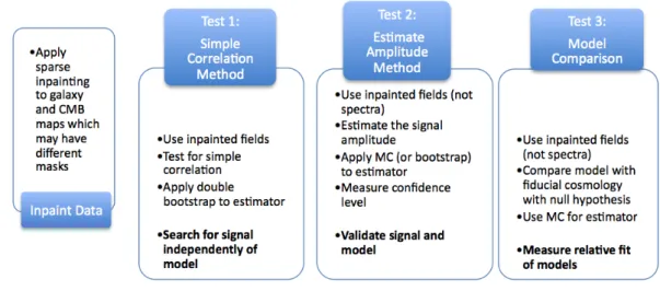
Having identified in the previous section the numerous methods used in the literature to detect and measure the ISW signal, as well as their relative advantages and disad-vantages, we propose here a complete and rigorous method for detecting and quantifying the signal significance. We describe this method in detail below and it is summarised in Figure 2.
4.1. Motivation
If we consider the pros and cons of each detection method shown in Table 2 and in Section 3.3, we remark first that any method based on the comparison of spectra makes the demanding assumption that the C(&)!s be Gaussian, whereas methods based on field comparison require only the primordial CMB field to be Gaussian. Instead the fields method assumes only that the primordial CMB is Gaussian, so we recommend this method be used for an ISW analysis.
−4 −3 −2 −1 0 1 2 3 4 0 0.05 0.1 0.15 0.2 0.25 0.3 0.35 0.4 0.45 0.5 Empirical distribution Normal distribution 2σ boundary (normal) 2.5σ boundary (empiric)
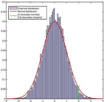
Fig. 1. Comparison of Gaussian PDF for estimator λ/σλwith its
true estimated distribution. A 2σ significance using the Gaussian PDF corresponds in fact to a 2.5σ detection with the true dis-tribution. (Calculation for 2MASS survey, see section 6).
Another key issue is the estimation of the signal sig-nificance. We find that most approaches in the literature assume that the probability distribution function (PDF) of the estimator is Gaussian. In Figure 1 we evaluate the esti-mator’s PDF (under the null hypothesis) for the ISW signal due the 2MASS survey (see Section 6) using a Monte-Carlo method (purple bars) and compare it with a Gaussian PDF (red solid line). The distributions’ tails differ which leads to a bias in the confidence level for positive data (i.e. data with an ISW signal). For the 2MASS survey, a 2σ detec-tion with a Gaussian assumpdetec-tion (vertical solid/green line) corresponds in fact to a 2.5σ detection using the true un-derlying PDF. In this case, the signal amplitude is under-estimated with the Gaussian assumption. Such behavior has also been studied for marginal detections by Bassett &
Afshordi (2010). To avoid this bias, we recommend that the PDF be estimated, and not assumed Gaussian.
Finally, there is not one ‘ideal’ statistical method. Different methods have both advantages and disadvantages and a combination of different methods can prove comple-mentary.
4.2. The Saclay method
We present here a new ISW detection method which uses the fields as input (and not the spectra). As we have seen, several statistical tests are interesting in the sense that they do not address the same questions. Therefore we believe that a solid ISW detection method should test:
1. The correlation detection: this test is independent of the cosmology.
2. The amplitude estimation: this will seek for a specific signal.
3. The model comparison: this allows us to check whether the model with ISW is preferred to the model without ISW.
Using the fields instead of the spectra means we must deal with the problem of missing data, which we solve with a sparse inpainting technique (see Appendix A). Such a method has already been applied with success for CMB lensing estimations (Perotto et al. 2010).
The last important issue is how we estimate the final detection level. As explained before, the z-score asymptot-ically follows a Gaussian distribution and so a bootstrap or Monte-Carlo method is required to derive the correct p-value from the true test distribution.
4.2.1. Methodology
Our optimal strategy (summarised by Figure 2) for ISW detection is the following:
1. Apply sparse inpainting to both the galaxy and CMB maps which may have different masks, essentially recon-structing missing data around the Galactic plane and bulge.
2. Test for simple correlation, using a double bootstrap (one to estimate the variance and another to estimate the confidence) and using the fields as input. This re-turns a model-independent detection level.
3. Reconstruct the ISW signal using expected cosmology and the inpainted galaxy density map.
4. Estimate the signal amplitude using the fields as input, and apply a bootstrap (or MC) to the estimator. This validates both the signal and the model.
5. Apply the model comparison test using the fields as in-put (see Section 4.2.2), essentially testing whether the data prefers a fiducial (e.g., ΛCDM) model over the null hypothesis, and measure relative fit of models.
As we have chosen to work with the fields, the very first step is to deal with the missing data. This is an ill-posed problem, which can be solved using sparse inpainting (see Appendix A for more details). This approach reconstructs the entirety of the field, including along the Galactic plane and bulge. We show in Section 5 that the use of sparse inpainting does not introduce a bias in the detection of the ISW effect.
Fig. 2. Description of the steps involved in our method for detecting the ISW effect. Tests 1 to 3 are complementary and ask different statistical questions.
We then perform a correlation detection on the re-constructed fields data using a double bootstrap (see Appendix B.1). Experiments show that the bootstrap tends to over-estimate the confidence interval, especially when the p-values are small. This is why the obtained detection must be used as a indicator when near a significant value (for high p-values, the bootstrap remains accurate).
The second test evaluates the signal amplitude, which validates both the presence of a signal and the chosen model. Bootstrapping test can also be used here as it has no assumption on the underlying cosmology. However, since the accuracy of bootstrap depends on the quantity of ob-served elements, it may become inaccurate for low p-value, i.e. when there is detection. In such case, Monte-Carlo (MC) will provide more accurate p-values and, for example, with 106MC simulations, we have an accuracy of about 1/1000.
This second test compares the ISW signal with a fidu-cial model, but does not consider the possibility that the measured signal could in fact be consistent with the ‘null hypothesis’. So even with a significant signal, a third test is necessary. This more pertinent question is addressed by using the ‘Model Comparison’ method (defined in Section 4.2.2), for the first time using the fields approach.
In conclusion, our method consists of a series of comple-mentary tests which together answer several questions. The first test seeks the presence of a correlation between two fields, without any referring cosmology. The second model-dependent test searches a given signal and tests its nullity. The third test asks whether the data prefers a fiducial ISW signal over the null hypothesis.
4.2.2. ‘Field’ model comparison
We define here the model comparison technique us-ing the fields approach, which has until now not been used in the literature. Using a generalised likeli-hood ratio approach, the quantity to measure is:
K6= δOBS∗ CT T−1δOBS−
(δISW− δOBS)∗CT T−1(δISW− δOBS) .
(24)
Theoretically K6 convergences asymptotically to a χ2
vari-able with a certain number of d.o.f ’s. As we only have one observation we cannot assume (asymptotic) convergence. We can however use a Monte Carlo approach in order to estimate the p-value of the test under the H0 hypothesis.
The p-value is defined as the probability that under H0
the test value can be over a given K6, i.e. P (t > K6) =
'∞
K6p(x)dx, where p is the probability distribution of the
test under the H0 hypothesis. By simulating primordial
CMB for a fiducial cosmology, these values can be easily computed. Then the p-value gives us a confidence on re-jecting the H0 hypothesis.
Notice that the same procedure for the p-value esti-mation can be applied on K4 (Equation 22), even on K1
(Equation 15) and K3 (Equation 17) for the power spectra
methods. We will further refer to this p-value estimation as the Monte-Carlo estimation, as we theoretically know the distribution under the null hypothesis, i.e. the primordial CMB is supposed to come from a Gaussian random process.
5. Validation of the Saclay Method
In order to validate the Saclay method, we estimate the detection level expected using WMAP 7 data for the CMB and 2MASS and Euclid data for the galaxy data (see section 6 for a description of WMAP and 2MASS data sets). We quantify the effect of the inpainting process on CMB maps with and without an ISW signal. We do this by simulating 2MASS-like and Euclid-like Gaussian and lognormal galaxy distributions and WMAP7-like Gaussian CMB maps (using cosmological parameters from Table 6) both with and without an ISW signal. We then apply our method to attempt a detection of the ISW signal. We do this both on full-sky maps as well as on masked data where we have reconstructed data behind the mask using the sparse inpainting technique (the masks we use are as de-scribed in 6.1 and 6.2).
For each simulation, we run the 3-step Saclay method. Except for the cross-correlation method where we use 100
iterations for the 2MASS-like and 1000 for Euclid-like simulations for the p-value estimation and 201 for the variance estimation (nested bootstrap), every other Monte-Carlo process was performed using 10 000 iterationsAll tests were performed inside the spherical harmonics do-main with ! ∈ [2, 100] for 2MASS and & = [2, 350] for a Euclid-like survey.
For the Euclid-like survey, we consider a galaxy distribution as defined in Amara & R´efr´egier (2007), with mean redshift zm = 0.8 and slopes
α = 2, β = 1.5. We reconstruct the ISW effect created by the projected galaxy distribution of the Euclid survey, by considering only one large redshift bin. In the future, it could be possible to refine such a reconstructed map by considering tomographic bins, or using information from the spectroscopic survey. As sky coverage maps are not yet avail-able for Euclid, we consider the same mask as for 2MASS and inpaint regions with missing data fol-lowing Section 6.3. We choose do to this, rather than simply assume a value for the fraction of sky covered (fsky), so as to consider more realistic
prob-lems relating to the shape of the mask, and to test our inpainting method.
5.1. Expected level of detection:
The expected detection levels (in units of σ) are reported in Table 3 (2MASS) and Table 4 (Euclid). Methods 1 − 3 correspond to the 3-step method described in Figure 2, where (b) and (MC) denote bootstrap and Monte Carlo evaluations of the variance and the p-value of the test. The p-values are converted as a σ value using the following for-mula:
s =√2 erf−1(1 − p) , (25) where p is the p-value, s the corresponding σ-score and erf−1 the inverse error function.
The 2MASS simulations (Table 3) show that we expect the same level of significance for an ISW de-tection, whether the mass tracer follows a Gaussian or a lognormal distribution. In either case the sig-nificance is low, around 1σ ± 1σ. This mean that for 2MASS-like survey, we have a signal to noise ratio (S/N) around 1σ. We see no major difference between the expected detection levels of M2 and M3. The only difference is for M1 (but there is still agreement with M2 and M3 within 1σ error bars) -this may be due to the fact that the bootstrap tech-nique is more efficient for Gaussian assumptions.
We also apply our method to CMB simulations with no ISW signal present (2 left columns of Table 3), and find a lower detection significance than when an ISW signal is present. This is true even when inpainting is used to recover missing data, showing that the inpainting method does not intro-duce spurious correlations.
In any case, all methods suggest it is difficult to detect the ISW signal with high significance using the 2MASS data as a local tracer of the matter distribution.
In Table 4, we show that an Euclid-like sur-vey, which is optimally designed for an ISW de-tection (see, Douspis et al. 2008), permits a much
Gaussian density
Method Monte-Carlo Bootstrap
Cross-Correlation (Equation 11) 0.46± 0.28 0.44± 0.35 Amplitude estimation (Equation 21) 0.44± 0.30 0.47± 0.33 Lognormal density
Method Monte-Carlo Bootstrap
Cross-Correlation (Equation 11) 0.39± 0.27 0.38± 0.31 Amplitude estimation (Equation 21) 0.41± 0.26 0.40± 0.30
Table 5. Expected p-values for inpainted maps of ISW signal for a 2MASS-like local tracer of mass using Monte-Carlo or boot-strap methods for the first two steps of the Saclay method.
higher detection than with a 2MASS survey. As with 2MASS simulations, we notice that M2 and M3 return similar detection levels, which are lower than M1. Inclusion of masked data reduced the sig-nificance, but our inpainting method does not intro-duce spurious correlations as inpainted maps with no ISW do not return a detection. For a Euclid-like survey with incomplete sky coverage, we can expect to show that the data prefers an ISW component over no dark energy (M3) at the 4.7σ level, and de-tect a cross-correlation signal at the ∼ 7σ level. We find no significant differences in the detection lev-els when the simulations are assumed lognormal or Gaussian.
We also investigate the performance of the wild boot-strap method for the confidence estimation. Table 5 shows the p-values estimated using Monte-Carlo procedure and wild bootstrap for the first two methods of the 3-step Saclay method. Notice that the bootstrap results are almost equiv-alent to Monte-Carlo ones. We find the bootstrap method wasn’t always reliable when the p-value becomes small, be-cause the precision of the bootstrap depends on both the number of bootstrap samples (as any MC-like process) and the number of observed elements. This last dependence makes the bootstrap uncertain when the detection is almost certain, that is why we consider the bootstrapped cross-correlation as an indicator that needs refinement when the results are very significant.
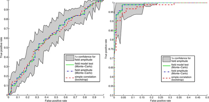
5.2. Power of the tests
In order to investigate the different strengths of each method, we also evaluate the rate of true positives vs. the number of false positives (i.e. false detections) - this infor-mation is summarised in Figure 3 which shows Receiver Operating Characteristic (ROC) curves. The construction of the ROC curve requires the computation of p-values for several simulated cases (i.e., simulations with and without an ISW signal), which are then sorted by value. For each p-value or threshold, the corresponding false positive and true positive rates are computed.
Generally, a more sensitive method may be more per-missive and so will return a higher proportion of false de-tections. An ideal method will have a ROC curve above the diagonal from (0, 1) to (1, 1). Similarly, a poor detector will produce a curve below the diagonal, which corresponds to
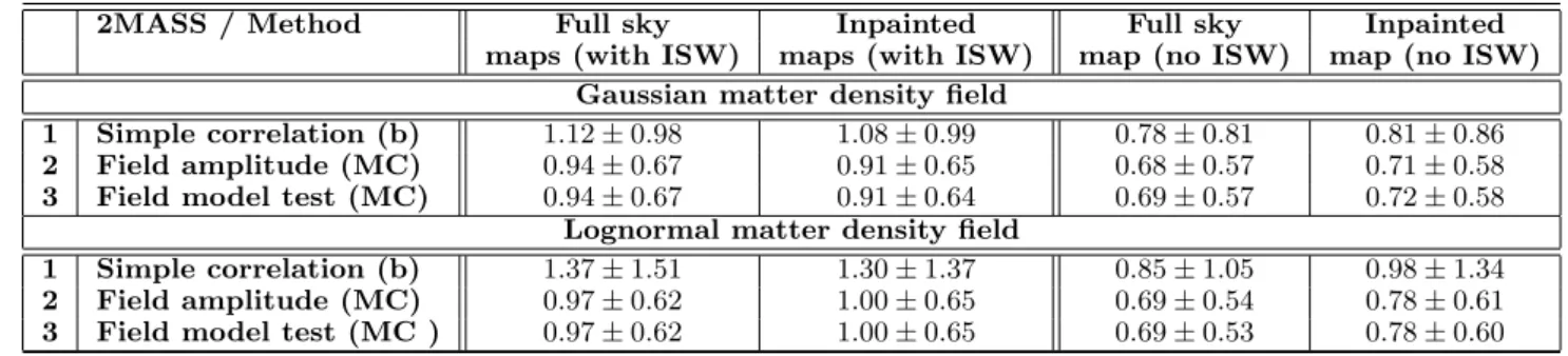
2MASS / Method Full sky Inpainted Full sky Inpainted
maps (with ISW) maps (with ISW) map (no ISW) map (no ISW)
Gaussian matter density field
1 Simple correlation (b) 1.12± 0.98 1.08± 0.99 0.78± 0.81 0.81± 0.86
2 Field amplitude (MC) 0.94± 0.67 0.91± 0.65 0.68± 0.57 0.71± 0.58
3 Field model test (MC) 0.94± 0.67 0.91± 0.64 0.69± 0.57 0.72± 0.58
Lognormal matter density field
1 Simple correlation (b) 1.37± 1.51 1.30± 1.37 0.85± 1.05 0.98± 1.34
2 Field amplitude (MC) 0.97± 0.62 1.00± 0.65 0.69± 0.54 0.78± 0.61
3 Field model test (MC ) 0.97± 0.62 1.00± 0.65 0.69± 0.53 0.78± 0.60
Table 3. Expected detection level (units of σ) of ISW signal for a 2MASS-like local tracer of mass assuming Gaussian and
lognormal distribution for a fiducial cosmology (see Table 6). Methods 1− 3 represent the 3-step method. Angular scales
included in the analysis are " = [2− 100].
Euclid / Method Full sky Inpainted Full sky Inpainted
maps (with ISW) maps (with ISW) map (no ISW) map (no ISW)
Gaussian matter density field
1 Simple correlation (b) > 7 6.98± 2.30 0.87± 0.67 0.99± 0.72
2 Field amplitude (MC) > 5 4.70± 2.40 0.78± 0.49 0.88± 0.54
3 Field model test (MC) > 5 4.77± 2.42 0.78± 0.48 0.88± 0.54
Lognormal matter density field
1 Simple correlation (b) > 7 6.29± 2.60 0.84± 0.70 0.77± 0.72
2 Field amplitude (MC) > 5 4.43± 2.37 0.75± 0.54 0.74± 0.54
3 Field model test (MC ) > 5 4.43± 2.37 0.74± 0.53 0.74± 0.54
Table 4. Expected detection level (units of σ) of ISW signal for a Euclid-like local tracer of mass assuming Gaussian
distribution for a fiducial cosmology (see Table 6). Methods 1− 3 represent the 3-step method. Angular scales
included in the analysis are " = [2− 300].
odds worse than tossing a coin. The X-axis corresponds to the false positive rate, i.e. the ratio of CMB maps without ISW where ISW signal is detected at the current threshold. The Y-axis corresponds to the true positive rate, i.e. the ratio of CMB maps with ISW where ISW signal is detected at the current. We recall that a point on the ROC curve corre-sponds to a threshold.
Figure 3 shows the ROC curves for three methods ap-plied to a 2MASS-like survey (Left) and a Euclid-like sur-vey (emphRight): fields model test (thin solid green), field amplitude estimation (dot-dashed blue), simple correlation (dashed red). For the 2MASS survey, all the methods are inside the 1σ error bar of the field’s amplitude estimation and so are nearly equivalent, i.e. no method performs better than the others.
For the Euclid-like survey, the statistics return much better values then for 2MASS (i.e., the ROC curves are far from the diagonal). The simple corre-lation method will return more false positives than the other two methods, which are nearly identical. The ROC curves for each method differ by more than 1σ at some points and so different methods will perform differently.
6. The ISW signal in WMAP7 due to 2MASS
galaxies
We apply the new detection method described in Section 4 to WMAP7 data (Jarosik et al. 2010) and the 2MASS galaxy survey which has been extensively used as a tracer of mass for the ISW signal (see Table 1).We describe first the data in Sections 6.1 and 6.2. In Section 6.3 we describe the
inpainting process that we apply to both CMB and galaxy data. In Section 6.4, we present the detection results. 6.1. WMAP
For the cosmic microwave background data, we use sev-eral maps from NASA Wilkinson Microwave Anisotropy Probe: the internal linear combination map (ILC) for years 5 and 7 (WMAP5, Komatsu et al. 2009) (WMAP7, Jarosik et al. 2010) and the ILC map by Delabrouille et al. (2009) which was reconstructed using a needlets technique. We avoid regions which are contaminated by Galactic emission by applying the Kq85 temperature mask - which roughly corresponds to the Kp2 mask from the third year release (see Figure 4). We also substract the kinetic Doppler quadrupole contribution from the data. WMAP sim-ulations used to produce Tables 3 and 4 use WMAP 7 best fit parameters for a flat ΛCDM universe (see Table 6).
Ωb 0.0449 Ωm 0.266 ΩΛ 0.734
n 0.963 σ8 0.801 h 0.710
τ 0.088 w0 -1.00 wa 0.0
Table 6. Best fit WMAP 7 cosmological parameters used throughout this paper.
6.2. 2MASS Galaxy Survey
The 2 Micron All-Sky Survey (2MASS) is a publicly avail-able full-sky extended source catalogue (XSC) selected in the near-IR (Jarrett et al. 2000). The near-IR selection
0 0.1 0.2 0.3 0.4 0.5 0.6 0.7 0.8 0.9 1 0 0.1 0.2 0.3 0.4 0.5 0.6 0.7 0.8 0.9 1
False positive rate
True positive rate 1! confidence for
field amplitude field model test (Monte!Carlo) field amplitude (Monte!Carlo) simple correlation (bootstrap) 0 0.05 0.1 0.15 0.2 0.25 0.3 0.35 0.4 0.45 0.5 0.5 0.55 0.6 0.65 0.7 0.75 0.8 0.85 0.9 0.95 1
False positive rate
True positive rate 1! confidence for
field amplitude field model test (Monte!Carlo) field amplitude (Monte!Carlo) simple correlation (bootstrap)
Fig. 3. ROC curves for the 3-step Saclay method for the 2MASS survey (Left) and the Euclid survey (Right). Note the axes in the right-hand panel are different than in the left-hand panel. The statistical methods correspond to: fields model test (thin solid green, Method 3 in Table 3), field amplitude estimation (dot-dashed blue, Method 2), simple correlation (dashed red, Method 1). For the 2MASS survey, all the methods are inside the 1σ error bar of the field’s amplitude estimation and so are nearly equivalent. For the Euclid-like survey, the statistics return much better values than for 2MASS (i.e., the ROC curves are far from the diagonal). The simple correlation method will return more false positives than the other two methods, which are nearly identical. The ROC curves of the simple correlation test differs sometimes by more than 1σ at some points from the other two methods and so is expected to perform differently.
Method Inpainted
maps (with ISW)
Simple cross-correlation (Eq. 13) 1.30σ± 1.37
Amplitude estimation (Eq. 22) 1.00σ± 0.65
Model selection (Eq. 23) 1.00σ± 0.65
Table 7. Expected detections for 2MASS like survey (from log-normal results in Table 3).
means galaxies are surveyed deep into the Galactic plane, meaning 2MASS has a very large sky coverage, ideal for detecting the ISW signal.
Following (Afshordi et al. 2004), we create a mask to exclude regions of sky where XSC is unreliable using the IR reddening maps of Schlegel et al. (1998). Using Ak = 0.367 × E(B − V ), Afshordi et al. (2004) find a limit
AK < 0.05 for which 2MASS is seen to 98% complete for
K20 < 13.85, where K20 is the Ks-band isophotal magni-tude. Masking areas with AK > 0.05 leaves 69% of the sky and approximately 828 000 galaxies for the analysis (see Figure 4).
We use the redshift distribution computed by Afshordi et al. (2004) (and also used in Rassat et al. 2007), and in order to maximise the signal, we consider one overall bin for magnitudes 12 < K < 14. The redshift distribution for 2MASS is that shown in Figure 1 of Rassat et al. (2007) (solid black line) and peaks at z ∼ 0.073. The authors also showed that the small angle approximation could be used for calculations relating to 2MASS, so Equations 10 and 4
can be replaced by their simpler small angle form: CgT(&) = − 3bH2 0Ωm,0 c3(& + 1/2)2 # drΘD2H[f − 1]P !& + 1/2 r " , (26) and Cgg(&) = b2 # drΘ2 r2D 2P !& + 1/2 r " (27) We estimate the bias from the 2MASS galaxy power spec-trum using the cosmology in Table 6 and find b = 1.27 ± 0.03, which is lower than that found in Rassat et al. (2007). 6.3. Applying Sparse Inpainting to CMB and Galaxy data As discussed in Section 4, regions of missing data in galaxy and CMB maps constitute an ill-posed problem when using a ‘field’ based method. We propose to use sparse inpainting (see Starck et al. 2010, and appendix A) to reconstruct the field in the regions of missing data.
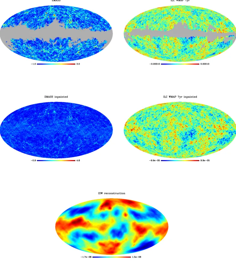
We apply this method to both the WMAP7 and 2MASS maps, and the reconstructed maps are shown in Figure 4. All maps are pixelised using the HEALPix software (G´orski et al. 2002; Gorski et al. 2005) with resolution correspond-ing to NSIDE=512. The top two figures show 2MASS data (left) and ILC map (right) with the masks in grey. The two figures in the middle show the reconstructed density fields for 2MASS data (left) and the ILC map (right). The bot-tom two figures show the reconstruction of the ISW field using the inpainted 2MASS density map and Equation 20 (for clarity, the first two multipoles (& = 0, 1) are not present in this map).
Fig. 4. Top: 2MASS map with mask (left) and WMAP 7 ILC map with mask (right). Middle: Reconstructed 2MASS (left) and WMAP 7 ILC (right) maps using our inpainting method. Bottom: reconstructed ISW temperature field due to 2MASS galaxies, calculated using Equation 20. For better visualisation of the maps as an input of the Saclay method, we consider only the information inside "∈ [2, 200].
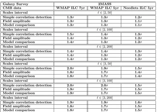
6.4. ISW Detection using 2MASS and WMAP7 Data We use the Saclay method (section 4) on WMAP7 and 2MASS data with 106 iterations for the Monte-Carlo
it-erations, 1000 iterations for both bootstrap and nested bootstrap of the correlation detection, and search for the ISW signal. In order to test the effect of includ-ing smaller (and possibly non-linear) scales, we perform the analysis for three different &-ranges: &∈ [&min, 50], [&min, 100], [&min, 200], where &min= 2 or 3.
We notice that inclusion or not of the quadrupole (& = 2) can affect the significance level slighty, which is why we chose two values for &min. We report our
mea-sured detection levels in Table 8. We recall the expected detections for 2MASS in Table 7, which can also be found in the more complete set of results presented in Table 3.
The results in Table 8 are compatible with the results in Table 3 within the errors bars. Rassat et al. (2007) used a spectra model-comparison method over & = [3 − 30], and found that the model with dark energy was marginally preferred over the null hypothesis. Over a range & = [2/3 − 50], using a fields model-comparison method, we find that a model with dark energy is preferred over the null hypothesis at the 1.1 − 1.8σ level, depending on the map. More generally, our results are compatible with the earliest ISW measurement using 2MASS data (Afshordi et al. 2004; Rassat et al. 2007) and lie in the 1.1 − 2.0σ range depending on the data and statistical test used.
The simple correlation test tends to report marginally higher detection levels than the field amplitude and model comparison tests, and the model comparison test similar values as the field amplitude test, which is compatible with the predictions from the ROC curves in Figure 3.
7. Discussion
In this paper we have extensively reviewed the numerous methods in the literature which are used to detect and mea-sure the presence of an ISW signal using maps for the CMB and local tracers of mass. We noticed that the variety of methods used can lead to different and conflicting conclu-sions. We also noted two broad classes of methods: one which uses the cross-correlation spectrum as the measure and the other which uses the reconstructed ISW tempera-ture field.
We identified the advantages and disadvantages of all methods used in the literature and concluded that:
1. Using the fields (instead of spectra) as input required only the primordial CMB to be Gaussian. This requires reconstruction of the ISW field, which is difficult with missing data.
2. The ill-posed problem of missing data can be solved using sparse inpainting, a method which does not introduce spurious correlations between maps. 3. Assuming the estimator was Gaussian led to
under-estimation of the signal under-estimation.
4. A series of statistical tests could provide complementary information.
This led us to construct a new and complete method for detecting and measuring the ISW effect. The method is summarised as follows:
1. Apply sparse inpainting to both the galaxy and CMB maps which may have different masks, essentially recon-structing missing data around the Galactic plane and bulge.
2. Test for simple correlation, using a double bootstrap (one to estimate the variance and another to estimate the confidence) and using the fields as input. This re-turns a model-independent detection level.
3. Reconstruct the ISW signal using expected cosmology and the inpainted galaxy density map;
4. Estimate the signal amplitude using the fields as input, and apply a bootstrap (or MC) to the estimator. This validates both the signal and the model.
5. Apply the fields model comparison test, essentially test-ing whether the data prefers a given model over the null hypothesis, and measure relative fit of models.
The method we present in this paper makes only one assumption: that the primordial CMB temper-ature field behaves like a Gaussian random field. The method is general in that it ‘allows’ the galaxy field to behave as a lognormal field, but does not automatically assume that the galaxy field is log-normal.
We first applied our method to 2MASS and Euclid simulations. We find that it is difficult to detect the ISW significantly using 2MASS simu-lations, and find no difference between assuming the underlying galaxy field is Gaussian or lognor-mal, and only mild differences depending on the statistical test used. With a Euclid-like survey, we expect high detection levels, even with incomplete sky coverage - we expect ∼ 7σ detection level us-ing the simple correlation method, and ∼ 4.7σ de-tection level using the fields amplitude or method comparison techniques. These detections levels are the same whether the Euclid galaxy field follows a Gaussian or lognormal distribution. Our results also show that the inpainting method does not in-troduce spurious correlations between maps.
We applied this method to WMAP7 and 2MASS data, and found that our results were comparable with early de-tections of the ISW signal using 2MASS data (Afshordi et al. 2004; Rassat et al. 2007) and lied roughly in the 1.1 − 2.0σ range. These results are also compatible with the simulations we ran for the 2MASS survey. The last test we performed, the model comparison test, asks the much more pertinent question of whether the data prefers a ΛCDM model to the null hypothesis (i.e. no cur-vature and no dark energy). Using this test, we find a 1.1 − 1.8σ detection for ranges & = [2/3 − 50] and 1.2 − 1.9σ for ranges & = [2/3 − 100/200], which is some-times higher than what was previously reported in Rassat et al. (2007) using a spectra models comparison test, without sparse inpainting or bootstrapping. A by-product of this measurement is the reconstruction of the temperature ISW field due to 2MASS galaxies, re-constructed with full sky coverage.
By applying our method on different estimation of the CMB map, we have highlighted the effect of the component separation on the ISW detection. Table 8 shows score between 1.1−2.0σ on that should be almost the same data, and with a previous test not reported here, we were able to detect ISW at