HAL Id: tel-01625202
https://tel.archives-ouvertes.fr/tel-01625202
Submitted on 27 Oct 2017
HAL is a multi-disciplinary open access archive for the deposit and dissemination of sci-entific research documents, whether they are pub-lished or not. The documents may come from teaching and research institutions in France or abroad, or from public or private research centers.
L’archive ouverte pluridisciplinaire HAL, est destinée au dépôt et à la diffusion de documents scientifiques de niveau recherche, publiés ou non, émanant des établissements d’enseignement et de recherche français ou étrangers, des laboratoires publics ou privés.
pre-processing well-logs
Pedram Masoudi
To cite this version:
Pedram Masoudi. Application of hybrid uncertainty-clustering approach in pre-processing well-logs. Earth Sciences. Université Rennes 1, 2017. English. �NNT : 2017REN1S023�. �tel-01625202�
0
ANNÉE 2017
Université de Téhéran
Collège d’Ingénierie Ecole des Mines
THÈSE / UNIVERSITÉ DE RENNES 1
sous le sceau de l’Université Bretagne Loire
En Cotutelle Internationale avec
Université de Téhéran, Iran
pour le grade de
DOCTEUR DE L’UNIVERSITÉ DE RENNES 1
Mention : Sciences de la Terre
Ecole doctorale Sciences de la Matière
présentée parPedram MASOUDI
Préparée à l’unité de recherche Géosciences-Rennes
CNRS UMR6118, Observatoire des Sciences de l’Univers de Rennes
Application of hybrid
uncertainty-clustering
approach in
preprocessing well-logs
Thèse rapportée par Behzad Tokhmechi
Université de North Dakota / rapporteur
Ali Kadkhodaie
Université de Curtin (Perth) / rapporteur
et soutenue à Téhéran le 16/05/2017
devant le jury composé de :
Ali Moradzadeh
Université de Téhéran / président
Kerry Gallagher
Université de Rennes 1 / examinateur
Mohsen Mohammadzadeh
Université de Tarbiat Modares / examinateur
Abolghasem Kamkar Rouhani
Université Technique Shahrood / examinateur
Omid Asghari
Université de Téhéran / examinateur
Dimitri Komatitsch
Université d’Aix-Marseille / examinateur
Tahar Aïfa
Université de Rennes 1 / directeur de thèse
Hossein Memarian
i To
my parents, Marjan and Hossein and
Dr. Hooshang Hakimi whom I owe a lot
« Faut-il rejeter toutes les probabilités parce qu'elles ne sont pas des certitudes? »
ii
Acknowledgments
First of all, the warmest thanks to my supervisors, Dr. Tahar Aïfa (University of Rennes 1), Dr. Hossein Memarian (University of Tehran) and my thesis tutor Dr. Behzad Tokhmechi (University of North Dakota) for their scientific advises.
Many thanks to the jury members of the proposal defense (Tehran 31/12/2014): Dr. Gholamhossein Norowzi, Mr. Hassan Madani, Dr. Omid Asghari and Dr. Ali Kadkhodaie-Illchi.
I also appreciate the jury members of the mi-parcours defense (Rennes 13/04/2016): Dr. Aline Dia, Dr. Jean-Noël Proust and Dr. Jean-Laurent Monnier.
Many thanks to the jury members of the final defense (Tehran 16/05/2017): Dr. Ali Moradzadeh, Dr. Kerry Gallagher, Dr. Mohsen Mohammadzadeh, Dr. Abolghasem Kamkar Rouhani, Dr. Omid Asghari, Dr. Dimitri Komatitsch, Dr. Behzad Tokhmechi, Dr. Ali Kadkhodaie, Dr. Tahar Aïfa and Dr. Hossein Memarian.
I would like to acknowledge Exploration Directorate of the National Iranian Oil Company for providing data and permitting the publication of scientific achievements. Thanks to the Research Unit of Geosciences-Rennes (CNRS UMR 6188) for the kind hospitality. Warm greetings to my friends in the Laboratory of Geo-engineering of School of Mining Engineering, University of Tehran for their kind help in accessing the computational and technical facilities of the laboratory remotely: Mr. Mohammadkhani, Mr. Amir Mollajan, Mr. Hossein Izadi, Miss Fatemeh Tavanaei, Mrs Atie Mazaheri and Mrs Farzaneh Khorram.
This work has been supported by the Center for International Scientific Studies and Collaboration (CISSC) and French Embassy in Iran through PHC GundiShapur 2016 program no. 35620UL. Kind thanks to other financial supports: The Cultural Institute of the Morality, Dr. Fereydoon Sahabi; Foundation of Dr. Mir-Mohammadi, Dr. Mir Saleh Mir Mohammadi and ZaminNegar Pasargad, Mr. Behzad SaeidBastami.
Pedram MASOUDI 20 May 2017
iii
Contents
Acknowledgments ... ii
Contents ... iii
List of figures ... vi
List of figures of appendices ... ix
List of tables ... x
Abstract ... 1
Résumé étendu ... 3
Graphical abstract ... 6
1 Introduction ... 7
Highlights of the Chapter 1 ... 7
1.1 Uncertainty resources in well-logging ... 7
1.2 The thesis questions and objectives ... 9
1.2.1 Question I: vertical resolution of well-logs ... 9
1.2.2 Question II: possibilistic uncertainty range of petrophysical parameters ... 12
1.3 The importance of the thesis ... 13
1.3.1 Fundamental and scientific importance ... 13
1.3.2 Application importance ... 13
1.3.3 Economic and management importance ... 13
1.4 Literature review ... 14
1.4.1 Uncertainty in sciences ... 14
1.4.2 Uncertainty in geosciences and petroleum exploration ... 16
1.5 Introducing datasets ... 21 1.5.1 Basic definitions ... 21 1.5.2 Synthetic data ... 22 1.5.3 Real data ... 22 2 Theories... 29 Highlights of Chapter 2... 29
2.1 Dempster-Shafer Theory of evidences ... 29
2.1.1 Body Of Evidences ... 30
2.1.2 Belief and plausibility functions ... 31
2.1.3 Consistency of uncertainty assessment theories ... 31
2.2 Fuzzy arithmetic ... 33
2.2.1 Fuzzy number ... 33
2.2.2 Arithmetic operations on intervals ... 35
2.2.3 Arithmetic operations on fuzzy numbers ... 35
2.3 Cluster analysis ... 36
2.3.1 k-means and fuzzy c-means algorithms ... 37
2.3.2 Gustafson-Kessel clustering technique ... 40
2.3.3 Gath-Geva clustering technique ... 40
2.4 Empirical relations in petrophysics ... 42
2.4.1 Porosity study by well-logs... 42
2.4.2 Irreducible water saturation ... 44
2.4.3 Wylie-Rose permeability relation ... 45
3 Modelling vertical resolution ... 47
Highlights of Chapter 3... 47
3.1 Volumetric nature of well-log recordings ... 47
iv
3.1.2 VRmf > spacing > sampling rate ... 49
3.2 Modelling logging mechanism by fuzzy memberships ... 50
3.2.1 Recording configuration and well-log ... 51
3.2.2 Approximating VRmf ... 52
3.2.3 Passive log of GR ... 57
3.2.4 Active logs of RHOB and NPHI ... 57
3.2.5 Complex membership function of compensated sonic log ... 58
3.3 Volumetric Nyquist frequency ... 60
3.4 Conclusions of Chapter 3 ... 64
4 Thin-bed characterization, geometric method ... 65
Highlights of Chapter 4... 65
4.1 Review of thin-bed studies ... 65
4.1.1 VLSA Method... 69
4.2 Theory of geometric thin-bed simulator ... 69
4.3 Sensitivity analysis of well-logs to a 30 cm thin-bed ... 73
4.4 Deconvolution relations for thin-bed characterization ... 76
4.5 Thin-bed characterization, the Sarvak Formation case-study ... 78
4.5.1 Multi-well-log thin-bed characterization ... 81
4.6 Conclusions of Chapter 4 ... 82
5 Enhancing vertical resolution of well-logs... 85
Highlights of Chapter 5... 85
5.1 Combining adjacent well-log records by Bayesian Theorem... 85
5.1.1 The importance of volumetric Nyquist frequency in up-scaling ... 87
5.2 Body Of Evidences (BOE) for well-logs ... 88
5.2.1 Focal elements of well-logs ... 88
5.2.2 Mass function of focal element of recording ... 89
5.3 Belief and plausibility functions for focal element of target ... 89
5.3.1 Theoretical functions of belief and plausibility ... 89
5.3.2 Geological constraints as an axiomatic structure ... 89
5.3.3 Practical functions of belief and plausibility... 91
5.3.4 Compensating shoulder-bed effect by epsilon ... 91
5.4 Log simulators... 92 5.4.1 Random simulator ... 92 5.4.2 Random-optimization simulator ... 92 5.4.3 Recursive simulator ... 94 5.4.4 Recursive-optimization simulator... 94 5.4.5 Validation criteria ... 94 5.5 The algorithm ... 95
5.6 Application check on synthetic cases... 97
5.7 Discussion on results of synthetic cases... 100
5.7.1 Validating constraint-based error by synthetic cases ... 101
5.8 Application to real data ... 102
5.8.1 Simulator selection ... 102
5.8.2 Optimizing factor of shoulder-bed effect... 103
5.8.3 Results of resolution improvement of real well-logs ... 103
5.9 Discussions ... 107
5.9.1 Comparing DST and geometry-based results in thin-bed characterization... 107
5.9.2 Advantages of DST-based algorithm ... 108
5.9.3 Uncertainty conversion using DST ... 109
5.10 Conclusions of Chapter 5 ... 110
6 Uncertainty projection on reservoir parameters... 112
Highlights of Chapter 6... 112
v
6.2 Porosity analysis by cluster-based method ... 114
6.2.1 Methodology of cluster-based porosity analysis ... 114
6.2.2 Results of cluster-based porosity analysis ... 119
6.2.3 Discussion of cluster-based porosity analysis ... 124
6.3 Permeability analysis by fuzzy arithmetic ... 127
6.3.1 Methodology of permeability analysis by fuzzy arithmetic ... 127
6.3.2 Validation with core data ... 129
6.3.3 Results and discussions of analysis by fuzzy arithmetic ... 130
6.4 Conclusions of Chapter 6 ... 133
7 Ending ... 139
7.1 Pathway of the thesis ... 139
7.1.1 Outlined achievements of the thesis ... 141
7.2 Recommendations ... 143
7.2.1 Recommendations for industrial applications... 143
7.2.2 Recommendations for further researches (perspectives) ... 143
References ... 145
Appendices ... 150
Appendix A: Convolution form of Relation 4-2 ... 150
Appendix B: Application check of DST-based simulators on synthetic-logs ... 150
Case 2: Deepening (fining) upward of GR ... 150
Case 3: Trough in RHOB ... 152
Case 4: Increasing upward of NPHI ... 153
Case 5: Peak in NPHI ... 154
Case 7: Fractured horizon in DT ... 155
Appendix C: Application check of random-optimization simulator on real well-logs ... 156
Well#2: 2766 – 2770 m ... 156
Well#3: 2809 – 2813 m ... 157
Well#4: 2662 – 2666 m ... 157
Well#5: 2840 – 2844 m ... 157
Appendix D: Publications and presentations of the thesis ... 159
vi List of figures
Figure 1-1. Schematic of basic concepts of logging: a) Vertical resolution of tool, membership function, depth of
investigation and assigning horizon. b) Overlap of adjacent records and sampling rate. ... 8
Figure 1-2. Using membership functions (right column) in representing a range of heterogeneity (lithology, porosity, etc.) of thin sections. ... 9
Figure 1-3. Conventional well-log interpretation. An example of rock typing (NikTab, 2003). ... 10
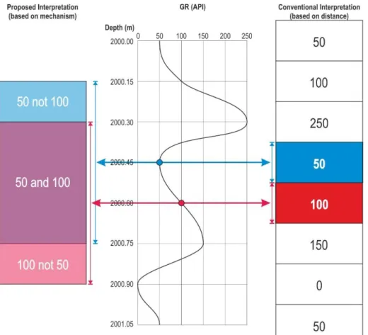
Figure 1-4. Comparing proposed and conventional interpretation approaches. Example of GR well-log. ... 11
Figure 1-5. The importance of fuzzy evaluation of well-logs in porosity evaluation. a) Porosity, based on well-log (left) and real values (right). b) VRmf, which is here proposed to be used instead of single value. The height is at 15% and its domain consists of all the possible porosity values. ... 12
Figure 1-6. Location of the field under study within the Abadan Plain, SW Iran. Modified after Sherkati and Letouzey (2004) and Rajabi et al. (2010)... 23
Figure 1-7. Lithostratigraphy of the Sarvak Formation and its neighbours (Dashtban, 2002). ... 25
Figure 1-8. a) Underground contour (UGC) map of the top Sarvak Formation in the study area. b) AA’ seismic section and its interpretation. c) Root mean square volumetric seismic amplitude attribute map, within 30 ms of the upper Turonian (the top Sarvak Formation, time slice of BCDE). The channelling of the top Sarvak Formation is shown on the FF’ seismic section (circle) (Abdollahie Fard et al., 2006). ... 26
Figure 1-9. Photos of the Sarvak Formation. a) Vugs on the top of Sarvak Formation, Siah-Kuh anticline, near Dehloran city, Ilam province (Masoudi et al. 2017). b) Weathering of the top Sarvak Formation, between Marv-Dasht (plain) and Takht-e Jamshid, Shiraz province. c) The unconformity: contact of the Sarvak and Ilam formations, Siah-Kuh anticline, near Dehloran city, Ilam province. ... 28
Figure 2-1. Comparing uncertainty assessment theories: probability (a) and DST (b). ... 30
Figure 2-2. Schematic examples of fuzzy numbers. ... 34
Figure 2-3. Fuzzy numbers for tidal ranges due to mean sea-level (Demicco and Klir, 2004). ... 34
Figure 2-4. Example of applying fuzzy operators on fuzzy numbers, integrated from Klir and Yuan (1995). ... 36
Figure 2-5. Flowchart of the FCM algorithm... 39
Figure 2-6. A snapshot of the spreadsheet for porosity estimation by the presented empirical relations. Vsh: shale volume, NPHIw, NPHIh, NPHIma and NPHIsh: NPHI in water, hydrocarbon, matrix and shale, respectively. NPHIm and PHInc are outputs (for NPHI) of Relations 2-26 and 2-27, respectively. RHOBw, RHOBh, RHOBma and RHOBsh: RHOB in water, hydrocarbon, matrix (2.65 g.cm-3 for calcite) and shale, respectively. PHId and PHIdc: are outputs (for RHOB) of Relations 2-26 and 2-27, respectively. PHIxdn, PHIxdn_Q and PHIxdn_CL are outputs of the methods density-neutron, quick-look and complex lithology, respectively. ... 45
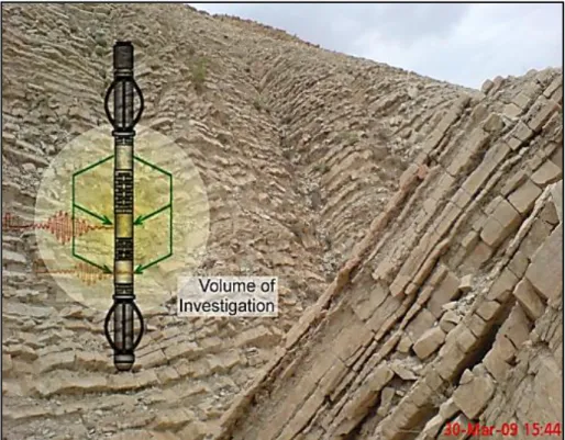
Figure 3-1. Schematic representation of volume of investigation around a sensor in a logging tool. ... 48
Figure 3-2. Depth of investigation and spacing of each well-log (Crain, 2000)... 48
Figure 3-3. The effect of an environment, out of the spacing, on the electrical logging. a) R1<R2: electric flow is getting away from the resistant environment (R2). b) R1=R2: electric flow is symmetrical. c) R1>R2: electric flow is getting closer to the conducting environment (R2). ... 50
Figure 3-4. Fuzzy membership function of contribution of each horizon in recording a passive (a) and an active (b) log. ... 51
Figure 3-5. Two possible configurations for detecting a thin-bed. Configuration B results in aliasing. In the well-logging, this phenomenon is called shoulder-bed effect, i.e. the effect of neighbouring beds. ... 52
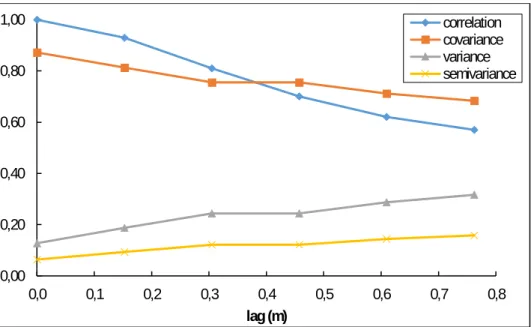
Figure 3-6. Cross-plots of adjacent recordings of GR (well#2)... 54
Figure 3-7. Measures of similarity (correlation and covariance) and dissimilarity (variance and semivariance) for adjacent recordings of GR in well#2. ... 54
Figure 3-8. Experimental variographs showing linear relation at the first lags. An open-source computer package, named The Stanford Geostatistical Modelling Software (SGeMS) is used to generate variographs. a) GR in well#2, b) RHOB in well#2, c) NPHI in well#3 and d) DT in well#5. ... 55
Figure 3-9. Comparison of VRmf with geological beds (Campbell, 1967), log-scale beds (Majid and Worthington, 2012), petrophysical beds (Passey et al., 2006). Modified after Passey et al. (2006). ... 56
vii
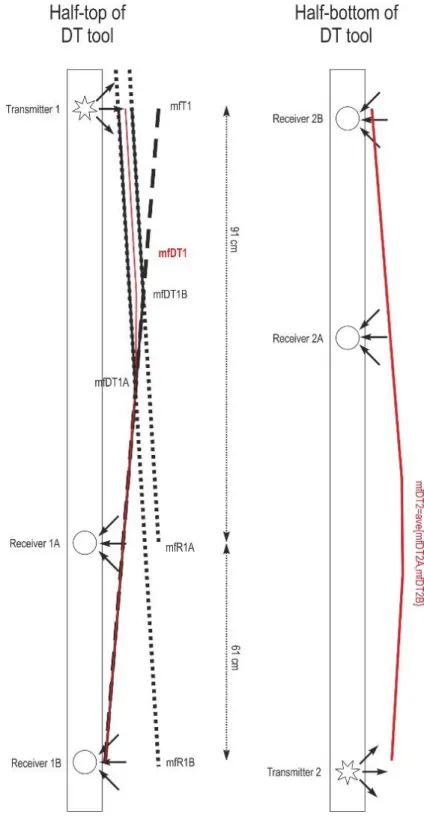
Figure 3-10. Mechanism of measurement of sonic transfer time by Borehole Compensated (BHC) sonic tool. Two transmitters and four receivers, finally fusing them by averaging (Close et al., 2009). Slowness=DT 58 Figure 3-11. Defined membership function for each half part of compensated sonic tool due to Figure 3-4b and
Table 1-4. ... 59 Figure 3-12. Calculated complex membership function for compensated sonic tool, by averaging membership
function of each half: a) theoretical and b) practical. ... 60 Figure 3-13. Nyquist frequency in three categories. Small balls are centre of recordings. a) Pulse-shapes
(VRmf=0) like in telecommunications, domain of time. Volumetric detection b) When 0<VRmf<SR or c) VRmf>SR. ... 61 Figure 3-14. Comparing probability of detecting a thin-bed without shoulder-bed effect, in three different
sensor types. In pulse-shape detections, VRmf=0, common Nyquist frequency is effective, i.e. the minimum thickness of a surely detectable thin-bed is SR. Volumetric detection when a) 0<VRmf<SR, dotted line or b) when VRmf>SR, dashed line. ... 62 Figure 3-15. Comparing belief function (pessimistic view) of detecting thin-beds without shoulder-bed effect, in three different sensor types. In pulse-shape detections, VRmf=0, common Nyquist frequency is effective, i.e. the minimum thickness of a surely detectable thin-bed is SR. Volumetric detection when a)
0<VRmf<SR, dotted line or b) VRmf>SR, dashed line. ... 63 Figure 4-1. Flowchart for hydrocarbon pore-thickness evaluation in thin-bed condition (Passey et al., 2006).
LCM stands for Log Convolution Modelling. Volumetric Laminated Sand Analysis (VLSA) is a probabilistic method, developed particularly to petrophysical evaluation of beds thinner than 1 ft (30 cm)... 68 Figure 4-2. a) Seven configurations in detecting a thin-bed when membership function is triangular. b) Details
of configuration III for calculating synthetic-log. ... 70 Figure 4-3. Sensitivity analysis and log response of random noise contamination: a) Sensitivity analysis of noisy
GR and b) synthetic GR with 0.5, 1, 1.5 and 2% noise. c) Sensitivity analysis of noisy RHOB and d) synthetic RHOB with 1%, 2%, 3% and 4% noise. e) Sensitivity analysis of noisy NPHI and f) synthetic NPHI with 1%, 2%, 5% and 10% noise. ... 75 Figure 4-4. Deconvolution results on synthetic data. a) Petrophysical values (NPHI) of thin-beds before (x) and
after (dot) reducing shoulder-bed effect. b) Thickness of thin-beds before (x) and after (dot) reducing shoulder effect. ... 78 Figure 4-5. Two examples of thin-bed interpretation on the real data. Thin-bed is firstly interpreted by the
well-logs individually. The well-log values are amplified and given on the thin-bed. Final thickness
interpretation and its associated uncertainty is provided in the rightmost track. a) Observation#7, well#1 (Table 4-3). b) A case-study in well#3, verified with the core box (yellow circles). The thin-bed
interpretation is inclined upward since the well-logs have an upward skewness. ... 83 Figure 5-1. PDFXn is a combination of n adjacent PDFs. SR=15.24 cm. a) VRmf=61 cm and b) VRmf=76 cm. ... 86 Figure 5-2. Defined focal elements of recording (𝐹𝐸𝑟) and target (𝐹𝐸𝑡) for a well-log with VRmf=4×SR. ... 88 Figure 5-3. Example of a well-log with vertical resolution of 91 cm (thick line), its average on five adjacent
points (dashed line) and the range between belief and plausibility (dotted lines). ɛ: compensating shoulder-bed effect at peaks and troughs only. ... 90 Figure 5-4. Scheme of the original well-log (solid line) and simulated-log (dashed line) within the uncertainty
range (grey). ɛ is multiplied by 5 (SE). The R3 should be a weighted average of S1 to S5 (white square) because they are within the 𝐹𝐸3𝑟 (hatched area). Due to assumptions of the algorithm, the distance should be compensated by S3. ... 93 Figure 5-5. Scheme of the processing. (a) Random-optimization and recursive-optimization simulators have to
pass through an optimization process, while the other more basic simulators only need a free or constraint-based random generation. (b) Flowchart of the DST-based algorithm for resolution
enhancement of well-logs. ... 98 Figure 5-6. a) Ideal-log, synthetic-log, uncertainty range and realizations of case 1. b) Error profiles: Comparison of constraint-based errors vs. depth between the simulators in case 1. c) Total error for 50 iterations. .. 99 Figure 5-7. Total constraint-based error during optimization in case 1. Convergence is reached at 6 and 12
epochs for random-optimization and recursive-optimization simulators, respectively. The term “epoch” refers to the number of iterations during the optimization process. To avoid confusion, the word
viii
Figure 5-8. Confusion matrix of correctness showing cases 1-5 and 7 and percentages. ... 101
Figure 5-9. Ideal-based vs. constraint-based error giving a significant correlation coefficient (R2). ... 102
Figure 5-10. Well-log (solid black line) data for the four tools (GR, RHOB, NPHI and DT), uncertainty range (blue zone), ten realizations (dots) and the best realization (dashed line) as the simulated-log, within the interval a) 3157-3159 m (well#1) and b) 2801.65-2803.45 m (well#3). ... 106
Figure 5-11. Uncertainty conversion by DST. The more depth uncertainty, the less value uncertainty. ... 110
Figure 6-1. Cross-plots of NPHI-RHOB (scaled) within the Sarvak Formation in well#3. RHOB is scaled to the range of NPHI, providing RHOB-based porosity estimation. a) Not clustered and b) clustered into five mass type clusters by FCM with inputs of NPHI, RHOB and DT. ... 113
Figure 6-2. Workflow of the algorithm of cluster-based porosity analysis. ... 115
Figure 6-3. FCM6 is trained on well-logs NPHI, RHOB and DT of well#3 (a). NPHI and core porosity of each cluster are compared through the cross-plot and histograms (b). ... 118
Figure 6-4. NPHI calibration for porosity estimation: removing the extremes of core porosity, then scaling PDF of NPHI to the new core porosity interval. ... 118
Figure 6-5. Results of cluster-based porosity analysis. When the core porosity is between the limits of clusters, the consistency mark is shown on the plot. Cluster limits in non-cored intervals are interpolated by the adjacent data. a) well#1, b) well#2, c) well#3, d) well#4 and e) well#5. fr: fraction. ... 123
Figure 6-6. Comparison of the RMSE of porosity estimation methods. ... 124
Figure 6-7. Generalization check of porosity estimators. ... 125
Figure 6-8. Homogeneous porosity zone within the Sarvak Formation. ... 126
Figure 6-9. Compatibility of core porosity with α-cuts (alfa-cuts). ... 129
Figure 6-10. Porosity analysis by fuzzy number. a) well#1, b) well#2, c) well#3, d) well#4 and e) well#5. fr: fraction. ... 131
Figure 6-11. Comparison of results of clustering-fuzzy arithmetic porosity analyses with VLSA method (based on Monte-Carlo simulation) by criterion 1 (a) and criterion 2 within well#1 (b), well#2 (c), well#3 (d), well#4 (e) and well#5 (f)... 132
Figure 6-12. Irreducible water analysis of fuzzy number. a) well#1, b) well#2, c) well#3, d) well#4 and e) well#5. fr: fraction. ... 134
Figure 6-13. Comparison of results of fuzzy arithmetic irreducible water analysis (wells #3 and #5) by criterion 1 (a) and criterion 2 (b). ... 135
Figure 6-14. Permeability analysis by fuzzy number: Morris-Biggs (left) and Timur (right) for Well#1 (a,b), well#2 (c,d), well#3 (e,f), well#4 (g,h), well#5 (i,j). ... 138
Figure 6-15. Comparing results of fuzzy arithmetic permeability analysis. ... 138
Figure 7-1. Larger the dimension, smaller the uncertainty range of measurements in petrophysical variables (here porosity). From this viewpoint, the uncertainty (also heterogeneity) has a statistical aspect. ... 140
ix List of figures of appendices
Figure A 1. a) Ideal-log, synthetic-log, uncertainty range, simulations (realizations) and the best realization of each simulator in case 2. Error comparison between the simulators: b) error profiles, and c) total error of
50 iterations. ... 151
Figure A 2. Same legend as in Figure A 1, case 3. ... 152
Figure A 3. Same legend as in Figure A 1, case 4. ... 153
Figure A 4. Same legend as in Figure A 1, case 5. ... 154
Figure A 5. Same legend as in Figure A 1, case 7. ... 155
Figure A 6. Well-log (solid line), uncertainty range, simulations (realizations, dots), and best realization (dashed line) in well#2. Correlation of well- and simulated-logs for perforation is marked by solid red and dashed green line, respectively. ... 156
Figure A 7. Well#3. Same descriptions as in Figure A 6. ... 157
Figure A 8. Well#4. Same descriptions as in Figure A 6. ... 158
x List of tables
Table 1-1. Sources of uncertainty in well-logs. ... 10
Table 1-2. Specifications of the ideal-logs to generate the synthetic logs. ... 22
Table 1-3. Available data within the Sarvak interval. #: number. GR: gamma ray, CGR: gamma ray of potassium, DT: sonic transfer time, NPHI: neutron porosity, RHOB: bulk density, DRHO: density correction, LLD: deep laterolog, LLS: shallow laterolog, MSFL: microspherically focused log, PEF: photoelectric effect. ... 23
Table 1-4. Details of the available well-logs in the field due to Schlumberger (2015). ... 24
Table 2-1. Consistency of BOEs with uncertainty assessment methodologies. ... 32
Table 2-2. Available axioms for the defined interval operators. Summarized from Klir and Yuan (1995). ... 35
Table 2-3. Suggested constants for Wylie and Rose (1950) permeability relation. ... 46
Table 3-1. Finding VRmf for each well-log, in each well by variography. VRmf is selected as minimum value of all the wells, larger values might be because of homogeneity of rocks. Units are in cm. ... 55
Table 3-2. Summary of designed membership functions of each log. ... 60
Table 3-3. Minimum thickness of beds to be characterized probably or surely. The uncertain interval showing an interval where probability is neither zero nor one. ... 64
Table 4-1. Defining reliable and risky windows for interpreting noisy well-logs, the case of 30 cm thin-bed. .... 75
Table 4-2. Comparing MSE of thin-bed characterization. Interpretations are based on synthetic-logs versus regression models (deconvolved) (Figure 4-4). ... 77
Table 4-3. Thin-bed characterizations of 10 real cases within Sarvak Formation, well#1. The apparent thickness values of the thin-beds are scaled to be closer to real thickness values by the deconvolution models. NAN: thin-bed curve not observed. ... 79
Table 5-1. Properties of constructed PDFs in Figure 5-1. ... 87
Table 5-2. Total errors of simulators for each synthetic case. Minimum errors are highlighted by bold characters. DST-based algorithm cannot detect a single fracture, case 6. ... 101
Table 5-3. Constraint-based total errors for the four simulators. SE=5 and iteration number=200. The reference for nfuse is the vertical resolution (Table 3-1). The parameters of simulation, including nfuse, are summarized in Table 5-5. ... 103
Table 5-4. Optimizing SE by comparing constraint-based total errors, iteration number=50. Larger iteration numbers are also tested, however the outputs were rubost. The parameters of the simulation (including SE) are mentioned in Table 5-5. ... 104
Table 5-5. Optimized parameters for random-optimization simulator. Summary of Table 5-3 and 5-4. ... 104
Table 5-6. Comparing the outputs of geometry- and DST-based algorithms in thin-bed characterization, the Sarvak Formation. The most accurate values in each row are given in bold characters. ... 107
Table 6-1. Comparing different algorithms and cluster numbers. The clustering algorithms are: k-means (KM), Fuzzy c-means (FCM), Gustafson-Kessel (GK) and Gath-Geva (GG). *Only one cluster is detected. **Only two clusters are detected. ^The clusters are intervened completely (due to the histogram) so the PM is unreliable. ... 116
Table 6-2. Batch optimization of removing core porosity extremes. The optimization is achieved on the best cases of Table 6-1. The calculated values are RMSE. ... 119
Table 6-3. Sequential optimization of removing core porosity extremes. The calculated numbers are RMSE. In each row, while the percentage of each cluster is changing, the other percentages are fixed. For the first row of each well, all the percentages are chosen based on the best optimization process of Table 6-2, then modified based on the best results of the previous row. ... 120
Table 6-4. Final removal percentages of each cluster for different estimators. ... 120
Table 6-5. Generalization ability of the estimators. ... 126
Table 6-6. Buckles number in each well, calculated from core data. ... 127
1
Abstract
In the subsurface geology, characterization of geological beds by well-logs is an uncertain task. The thesis mainly concerns studying vertical resolution of well-logs (question 1). In addition, fuzzy arithmetic is applied to experimental petrophysical relations to project the uncertainty range of the inputs to the outputs, here irreducible water saturation and permeability (question 2). Regarding the first question, the logging mechanism is modelled by fuzzy membership functions. Vertical resolution of membership function (VRmf) is larger than spacing and sampling rate. Due to volumetric mechanism of logging, volumetric Nyquist frequency is proposed.
Developing a geometric simulator for generating synthetic-logs of a single thin-bed enabled us analysing sensitivity of the well-logs to the presence of a thin-bed. Regression-based relations between ideal-logs (simulator inputs) and synthetic-logs (simulator outputs) are used as deconvolution relations for removing shoulder-bed effect of thin-beds from GR, RHOB and NPHI well-logs. NPHI deconvolution relation is applied to a real case where the core porosity of a thin-bed is 8.4%. The NPHI well-log is 3.8%, and the deconvolved NPHI is 11.7%. Since it is not reasonable that the core porosity (effective porosity) be higher than the NPHI (total porosity), the deconvolved NPHI is more accurate than the NPHI well-log. It reveals that the shoulder-bed effect is reduced in this case. The thickness of the same thin-bed was also estimated to be 13±7.5 cm, which is compatible with the thickness of the thin-bed in the core box (<25 cm). Usually, in situ thickness is less than the thickness of the core boxes, since at the earth surface, there is no overburden pressure, also the cores are crushed.
Dempster-Shafer Theory (DST) was used to create well-log uncertainty range. While the VRmf of the well-logs is more than 60 cm, the VRmf of the belief and plausibility functions (boundaries of the uncertainty range) would be about 15 cm. So, the VRmf is improved, while the certainty of the well-log value is reduced. In comparison with geometric method, DST-based algorithm resulted in a smaller uncertainty range of GR, RHOB and NPHI logs by 100%, 71% and 66%, respectively.
2
In the next step, cluster analysis is applied to NPHI, RHOB and DT for the purpose of providing cluster-based uncertainty range. Then, NPHI is calibrated by core porosity value in each cluster, showing low RMSE compared to the five conventional porosity estimation models (at least 33% of improvement in RMSE). Then, fuzzy arithmetic is applied to calculate fuzzy numbers of irreducible water saturation and permeability. Fuzzy number of irreducible water saturation provides better (less overestimation) results than the crisp estimation. It is found that when the cluster interval of porosity is not compatible with the core porosity, the permeability fuzzy numbers are not valid, e.g. in well#4. Finally, in the possibilistic approach (the fuzzy theory), by calibrating α-cut, the right uncertainty interval could be achieved, concerning the scale of the study.
Keywords: well-log uncertainty, vertical resolution, volumetric Nyquist frequency, thin-bed
3
Résumé étendu
Application de l'approche hybride incertitude-partitionnement pour le prétraitement des données de diagraphie
Dans la géologie de subsurface, la caractérisation des couches minces par les diagraphies est accompagnée d’incertitudes. Les sources de ces incertitudes proviennent des enregistrements discontinus (échantillonnage numérique), de l’acquisition volumétrique des données, des aspects techniques, etc. La thèse est principalement centrée sur l’étude de la résolution verticale des diagraphies (question 1). Dans la deuxième étape, l’arithmétique floue est appliquée aux modèles expérimentaux pétrophysiques en vue de transmettre l’incertitude des données d’entrée aux données de sortie, ici la saturation irréductible en eau et la perméabilité (question 2). Afin de résoudre les questions sus-jacentes, on a appliqué les théories de Dempster-Shafer (DST), d’arithmétique floue, d’analyse de regroupement des données et les expressions empiriques pétrophysiques.
Les diagraphies sont des signaux digitaux dont les données sont des mesures volumétriques. Le mécanisme d’enregistrement de ces données est modélisé par des fonctions d’appartenance floues (fuzzy membership functions). On a montré qu’il y avait trois types de résolution verticale pour les diagraphies : (i) le taux d’échantillonnage, (ii) l’espacement et (ii) la Résolution Verticale de la Fonction d’Appartenance (VRmf). Ils sont toujours en ordre descendant : VRmf>espacement>taux d’échantillonnage. Dans l’étape suivante, la fréquence de Nyquist est revue en fonction du mécanisme volumétrique de diagraphie ; de ce fait, la fréquence volumétrique de Nyquist est proposée afin d’analyser la précision des diagraphies.
Basé sur le modèle de résolution verticale développée, un simulateur géométrique est conçu pour générer les registres synthétiques d’une seule couche mince. Le simulateur nous permet d’analyser la sensibilité des diagraphies en présence d’une couche mince. Les relations de régression entre les registres idéaux (données d’entrée de ce simulateur) et les registres synthétiques (données de sortie de ce simulateur) sont utilisées comme relations de déconvolution en vue d’enlever l’effet des épaules de couche (shoulder-bed effect ou l’effet des couches voisines) d’une couche mince sur les diagraphies GR, RHOB et NPHI. Les relations
4
de déconvolution ont bien été appliquées aux diagraphies pour caractériser les couches minces. Par exemple, pour caractériser une couche mince poreuse, on a eu recours aux données de carottage qui étaient disponibles pour la vérification : NPHI mesuré (3.8%) a été remplacé (corrigé) par 11.7%. NPHI corrigé semble être plus précis que NPHI mesuré, car la diagraphie a une valeur plus grande que la porosité de carottage (8.4%). Il convient de rappeler que la porosité totale (NPHI) ne doit pas être inférieure à la porosité effective (carottage). En plus, l’épaisseur de la couche mince a été estimée à 13±7.5 cm, compatible avec l’épaisseur de la couche mince dans la boite de carottage (<25 cm). Normalement, l’épaisseur in situ est inférieure à l’épaisseur de la boite de carottage, parce que les carottes obtenues ne sont plus soumises à la pression lithostatique, et s’érodent à la surface du sol.
La Théorie de l’évidence de Dempster-Shafer (DST) est appliquée aux diagraphies. Le Corps Des Evidences (BOE) est défini à partir du mécanisme de diagraphie : si la diagraphie est considérée comme la fonction de masse, les éléments de références (focal elements) seraient les volumes d’investigation. Ensuite, les fonctions de croyance (belief ou probabilité inférieure) et de plausibilité (probabilité supérieure) sont calculées pour l’intersection de quatre ou cinq enregistrements adjacents de diagraphie. Par conséquent, l’intervalle d’incertitude de DST sera entre les fonctions de croyance et de plausibilité. Tandis que la VRmf des diagraphies GR, RHOB, NPHI et DT est ~60 cm, la VRmf des fonctions de croyance et de plausibilité est ~15 cm. Or, on a perdu l’incertitude de la valeur de diagraphie, alors que la VRmf est devenue plus précise.
Les diagraphies ont été ensuite corrigées entre l’intervalle d’incertitude de DST avec quatre simulateurs. Les hautes fréquences sont amplifiées dans les diagraphies corrigées, et l’effet des épaules de couche est réduit. La méthode proposée est vérifiée dans les cas synthétiques, la boite de carottage et la porosité de carotte. Les incertitudes de DST sur les diagraphies GR, RHOB et NPHI sont respectivement de 100%, 71% et 66%, donc inférieures à celles calculées par la méthode géométrique.
L’analyse de partitionnement (cluster analyses) est appliquée aux diagraphies NPHI, RHOB et DT en vue de trouver l’intervalle d’incertitude, basé sur les grappes. Puis, le NPHI est calibré par la porosité de carottes dans chaque grappe. Le RMSE de NPHI calibré est plus bas par
5
rapport aux cinq modèles conventionnels d’estimation de la porosité (au minimum 33% d’amélioration du RMSE). Le RMSE de généralisation de la méthode proposée entre les puits voisins est augmenté de 42%.
L’intervalle d’incertitude de la porosité est exprimé par les nombres flous (fuzzy numbers). L’arithmétique floue (fuzzy arithmetic) est ensuite appliquée dans le but de calculer les nombres flous de la saturation irréductible en eau et de la perméabilité. Le nombre flou de la saturation irréductible en eau apporte de meilleurs résultats en termes de moindre sous-estimation par rapport à l’estimation nette (crisp). Il est constaté que lorsque les intervalles de grappes de porosité ne sont pas compatibles avec la porosité de carotte, les nombres flous de la perméabilité ne sont pas valables, ex. du puits#4.
Enfin, pour les études géologiques, il est suggéré de considérer « l’échelle de l’étude » à côté d’autres conditions préalables de l’évaluation de l’incertitude, c’est-à-dire le but de l’étude et les sources de l’incertitude. Etant donné les trois conditions préalables, on peut choisir notre approche de l’évaluation de l’incertitude, puis choisir une théorie, donc une méthodologie. Un avantage qu’apporte la théorie possibiliste est que la coupure α (α-cut) peut être calibrée pour atteindre un intervalle de l’incertitude approprié, correspondant à l’échelle de l’étude.
Mots-clés : incertitude de diagraphie, résolution verticale, fréquence volumétrique de
6
7
1 Introduction
Highlights of the Chapter 1
Volumetric mechanism of well-logging is one of the uncertainty sources of vertical resolution. The first objective of the thesis is to model the vertical resolution of well-logs.
The second objective is to calculate a possibilistic uncertainty range of petrophysical interpretations, derived from well-logs.
Due to the literature, the goal of the study and the sources of uncertainty have to be addressed for all the uncertainty assessment studies.
1.1 Uncertainty resources in well-logging
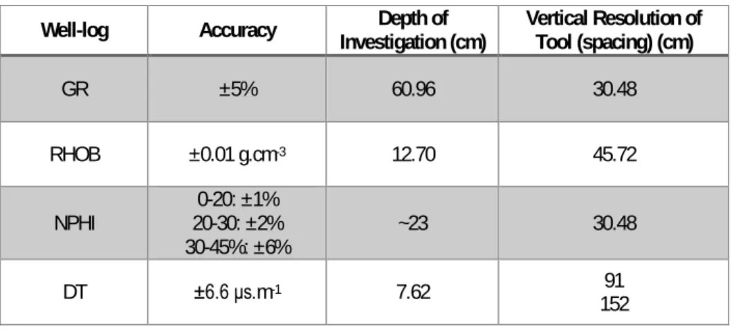
Well-log is a digital signal, acquired through a drilled well. It represents some properties (petrophysical, geometrical and sometimes geochemical) of the wellbore. Comparing to the other subsurface data, i.e. cores and well-tests, well-logs are more available, denser and more continuous. The sampling rate in well-logs is about 15 cm, however each sample belongs to a volume of investigation with the dimension of about 7- 160 cm (Schlumberger, 2015). The larger the dimension of the volume of investigation, the less precise the acquired data. Thin-bed problem arises when the Thin-beds are thinner than the vertical dimension of volume of investigation of the tool.
Resolution of well-logs could be discussed vertically or horizontally. Horizontal resolution is equivalent to the depth of investigation, and vertical resolution can be defined by: (i) sampling rate, (ii) Vertical Resolution of Tool (VRT) or spacing between transmitter and transducer, and
(iii) domain of Vertical Resolution of membership function (VRmf) (Figure 1-1).
VRmf shows the degree of membership of the volume of investigation to each property value (Masoudi et al., 2017). When the sample under study is completely homogeneous, VRmf could
8
be replaced by a single value. However when the heterogeneity rises, wider windows have to be used (Figure 1-2).
(a) (b)
Figure 1-1. Schematic of basic concepts of logging: a) Vertical resolution of tool, membership function, depth of investigation and assigning horizon. b) Overlap of adjacent records and sampling rate.
In addition to the resolution problem, like all the sensory data, well-logs are noise contaminated: white and coloured noises. White noise is a part of a signal (in frequency domain) that is weakly stationary, zero mean and uncorrelated (Gray and Lee, 2007). It contains usually high-frequencies, so resembles random behaviour. The associated white noise of each instrument is provided within the catalogues of the logging tools, like in Schlumberger (2015). Coloured noise is biased, low-frequency, and is related to the environmental changes, like temperature and pressure. Since the coloured noise is not random and its source is known, it is possible to remove (or to reduce) the effect of coloured noises, e.g. correcting gamma well-log
9
by removing the effect of mud-weight on the measurements. All the explained sources of uncertainty in well-logs, are summarized in Table 1-1.
Figure 1-2. Using membership functions (right column) in representing a range of heterogeneity (lithology, porosity, etc.) of thin sections.
1.2 The thesis questions and objectives
1.2.1 Question I: vertical resolution of well-logs
In conventional well-log interpretations (Figure 1-3), each depth is interpreted according to the nearest well-log record, could be named distance-based interpretation. The mechanism of well-logging is not taken into account, and we think that this approach is not the most precise way of interpreting well-logs. Instead of assigning each depth to the nearest well-log record,
10
we try to assign each well-log record to the domain of VRmf (Figure 1-4). Regarding this general idea, two questions are introduced to be discussed within the thesis.
Table 1-1. Sources of uncertainty in well-logs.
Measurement aspect Source of uncertainty Studies
Intrinsic randomness of nature - High complexities and heterogeneities in the nature
Kitts (1976)
Depth of measurement - Cable stretch
- Logging while moving the instrument
- Speed of logging
Passey et al. (2006)
Depth of investigation Volumetric measurement Vertical Resolution of Tool
(VRT) Volumetric measurement Flaum et al. (1989) Galford et al. (1989) Gartner (1989) Flaum (1990)
Vertical Resolution of
membership function (VRmf) Volumetric measurement Masoudi et al. (2017)Passey et al. (2006): under the name of absolute resolution Sampling rate Digital recording Passey et al. (2006)
Error of measurement, precision and white noise
Sensors and tools Gimbe (2015) Bardy (2015)
Coloured noise: environmental
effects - Temperature - Pressure - Mud weight - Borehole breakout - etc.
Processing, calibration and interpretation
- Imprecise concepts
- Incomplete subsurface information, - Human error
- etc.
Moore et al. (2011) Passey et al. (2006) Bardy (2015)
11
Figure 1-4. Comparing proposed and conventional interpretation approaches. Example of GR well-log.
The sources of uncertainty in well-log data is introduced in the previous part. Each source, Table 1-1, adds its specific uncertainty range to the well-log value. The first question, going to be addressed, is assessing VRmf. The absolute resolution of well-logs is a function of specific tool’s intrinsic resolution, sampling rate, logging speed and processing method (Passey et al., 2006). However in this thesis, this question primarily concerns the uncertainty of unprocessed data. Consider that a porosity well-log, e.g. neutron porosity (NPHI), is acquired over a range of real porosities (Figure 1-5a). The well-log shows 10% porosity, however the acquisition is taken place over a volume of investigation with the porosity range of [0%, 50%]. Even the height of the membership function is not necessarily equal to the well-log value. In this example, membership degree of the well-log value is higher than 0.9 (Figure 1-5b). The first objective is thus “to approximate VRmf of well-logs.”
12
(a) (b)
Figure 1-5. The importance of fuzzy evaluation of well-logs in porosity evaluation. a) Porosity, based on well-log (left) and real values (right). b) VRmf, which is here proposed to be used instead of single value. The height is at 15% and its domain consists of all the possible porosity values.
1.2.2 Question II: possibilistic uncertainty range of petrophysical parameters
The uncertainty range of acquired data should be propagated to the output of processed data and interpretations. So, the output (porosity, permeability, etc.) will have an uncertainty range, originated from the input well-logs. Therefore, the second objective of the thesis is “to calculate
possibilistic uncertainty range of petrophysical parameters, derived from well-logs.” The
uncertainty range is called “possibilistic” not to be confused with the uncertainty range of Monte-Carlo simulation, which is a “probabilistic” method. Also, from mathematical point of view, the possibilistic uncertainty range is a fuzzy measure, like in the Theory of Possibility, and not a Probability Distribution Function (PDF).
The well-logs gamma ray (GR), bulk density (RHOB), neutron porosity (NPHI) and sonic (DT) are chosen to apply the first objective on. For the second objective, porosity is studied comprehensively, permeability and water saturation are checked as well.
13 1.3 The importance of the thesis
1.3.1 Fundamental and scientific importance
Well-logs are subsurface data, acquired from hundreds of meters up to about four kilometres. Therefore, precision and accuracy of the data is under doubt, and it is basically necessary to investigate the uncertainty of these data.
In addition, the volume of investigation is overwhelmed in the common well-log interpretations (Figure 1-4). In the proposed methodologies, the role of depth uncertainty is also considered in the interpretations.
The proposed methods are based on the theories of Dempster-Shafer, clustering and fuzzy logic, which are specialized for data processing in uncertain situation. Developing these utilities in a new domain, here petroleum geology, is another scientific contribution of the thesis.
1.3.2 Application importance
The first necessity of studying uncertainty is in identifying the main uncertainty sources, and quantifying their relative importance (Dromgoole and Speers, 1997). As an example, in Lia
et al. (1997), two uncertainty sources associated in modelling reservoir production forecast are
introduced: (i) heterogeneity uncertainty, caused by geometrical arrangement; (ii) model parameter uncertainty because of incomplete knowledge of the whole reservoir properties. In this study, it is shown that heterogeneity uncertainty causes 25% of the total uncertainty, while model parameter uncertainty causes 75% of the whole uncertainty.
The importance of this thesis for the petroleum industry is to improve the vertical resolution of well-logs. The improved well-logs could be used for better characterization of the thin-beds.
1.3.3 Economic and management importance
The term “exploration” is defined idealistically as “a series of investment decisions made with decreasing uncertainty” (Rose, 1987). It shows the close relation of both concepts of
14
“uncertainty” and “decision-making”. Based on Megill (1979), the “Risk” is “an opportunity for loss”, and the “uncertainty” is defined as “the range of probabilities that some condition may exist or occur” (Rose, 1987).
Rose (1987) also introduced two criteria for continuing an exploration activity: (i) consistency with the strategy of investor in dealing with risk and uncertainty; (ii) understanding uncertainty accurately, and reducing it if possible. Meanwhile investors must cope with the issue of “risk” to come to reasonable decisions, engineers have to solve the problem of “uncertainty” to provide as clear illustration from the prospect as they can. In an uncertain situation (related to the exploratory activities), there are several biasedness: (i) prospect target size, (ii) discovery probability, and (iii) cost of finding.
From the economical viewpoint, the uncertainty is divided into two parts: risk and immaterial. Immaterial refers to those uncertainties, unimportant to business, whereas risk refers to the uncertainty of which is critical for business. Again, risk is classified into two types: opportunity and threat. The threat reflects risky uncertainties, threatening the enterprise, while the opportunity risk is a risky uncertainty, which might cause opportunities to the business (Smalley et al., 2008).
“Uncertainty is the only certainty in oil exploration.” It is a famous cliché in oil business (Fang and Chen, 1990). Lack of certainty in exploratory activities associates risk in investments. The terminology of “Responsible Reporting” is discussed in McLane et al. (2008), comprehensively. It discusses that an understanding of uncertainty is necessary for responsible reporting.
1.4 Literature review
1.4.1 Uncertainty in sciences
Philosophical debate on the concept of “uncertainty” backs to “skepticism”. Pyrrho (270-360 BC), who is rendered as being the first skeptic philosopher, reached to this idea that nothing is certain. So, his students and followers did not cry on his death because they did not believe
15
his death (Durant, 1953). Empiricism (observation) and rationalism (skepticism included) are two complementary or competing views in the epistemology. The former emphasizes on the importance of sensory data, while the latter concerns reasoning and certainty of human’s knowledge.
The debate on certainty of sensory data is not restricted to schools of philosophy. Maybe Thomas Bayes (mathematician and philosopher, lived between 1701 and 1761) is the first scientist who entered the concept of uncertainty in statistics and mathematics by his famous theory of probability. Another historic and well-known measure of uncertainty in mathematics and statistics is “variance”, which shows how data (or simulations) are distributed around a center. Also, error bar is a conventional tool for expressing uncertainty range as in Wong (2003).
Since then, the concept of uncertainty gradually entered in different applications, amongst electronics and telecommunication have benefited the most, by the development of “Information Theory” (Shannon, 1948). Shannon relation of uncertainty is the development of works of Harry Nyquist and Ralph Hartley in the Bell System Company, with the aim of development of communicating systems. Shannon’s formula is so fundamental that nowadays it is a famous measure of uncertainty in different domains of science as geosciences.
Scientists of electronics were pioneer in development of another theory in assessing uncertainty: Theory of Fuzzy, which was a paradigm shift in electronics. Generalizing the Set Theory, Zadeh (1965) introduced a new language for expressing membership of an element to a definite set. Instead of using two values (0 or 1) for indicating membership of an element, he used a membership function that its output could be within the interval of [0, 1] (Zadeh, 1965). These days, fuzzy logic is used vastly in various fields of science and engineering, and in geology as well (Demicco and Klir, 2004). Based on the concept of fuzziness, clustering algorithms were modified to develop fuzzy clustering tools, in order to use membership functions in stating degree of membership of data to clusters. Review of fuzzy clustering methods could be found in Baraldi and Blonda (1999), Krishnapuram and Keller (1993)and Pal et al. (2005). A review of possibilistic, fuzzy and neural models is also presented in Bezdek (1993).
16
Researchers of statistics and artificial intelligent were able in developing a rival for fuzzy logic. Dempster-Shafer Theory (DST) of evidences is another methodology in evaluating data within uncertain situation. By means of defining “mass function”, researchers were able in further developing Bayes rule to Dempster rule of combination to fuse output of multi-sensory detections under uncertain condition (Dempster, 1967, 1968; Shafer, 1976, 1990).
1.4.2 Uncertainty in geosciences and petroleum exploration
Intrinsic randomness of nature is perhaps the first source of uncertainty that is mentioned in geological texts. However, retrodiction is never as uncertain as prediction (Kitts, 1976). The word “retrodiction” could be of interest of geologists since it is composed of the word “prediction” when the prefix “pre” is replaced by “retro”.
Another pioneer work on uncertainty assessment in core orientation could be found in Nelson et al. (1987). In quantifying uncertainty in petroleum volume estimation, fuzzy arithmetic (Theory of Possibility) is declared to provide better results, comparing to Monte-Carlo method (Theory of Probability) (Fang and Chen, 1990). Monte-Carlo simulation is a traditional technique for calculating uncertainty of estimated hydrocarbon volume. For further study about probabilistic Monte-Carlo method, refer to Hurst et al. (2000) and Masoudi et al. (2011).
The uncertainty is categorized into two types: vagueness (equivalent to fuzziness, haziness, cloudiness, unclearness and sharplessness) and ambiguity (non-specificity, diversity, divergence, generality, variety and one-to-many). Three sources of uncertainty are introduced: lack of information, intrinsic nature and ignorance (Fang and Chen, 1990).
In a comprehensive study, fuzzy aggregation is used for reservoir appraisal (Chen and Fang, 1993). In this work, four trap properties (type, size, closure and timing), five reservoir properties (porosity, permeability, net thickness, depth and saturation), five source rock properties (richness, organic matter, maturity, thickness and area), migration distance and seal integrity, i.e. 16 geologic variables in overall, are fused to assess prospects. In brief, an appraisal method is introduced in this paper, which uses fuzzy aggregation methodology to easily integrate different reservoir properties.
17
Foley et al. (1997) classified uncertainty into three categories: fuzziness, randomness and incompleteness. Incompleteness is equivalent to ignorance, which is one of the sources of uncertainty, introduced in the work. Some authors also classified incompleteness into four categories: (i) what we know but have not included in the model; (ii) what we know that we do not know; (iii) what we do not know that we are unaware of it; and finally (iv) what is difficult to understand.
The concept “geoscore” was introduced by Dromgoole and Speers (1997) to measure the complexity of petroleum reserves by quantifying nine categories:
Structural complexity: (i) overburden complexity; (ii) fault complexity;
Reservoir quality and architecture: (iii) reservoir layering; (iv) reservoir continuity; (v) permeability channels; (vi) barrier continuity; (vii) fault transmissibility; (viii) fractures and
(ix) diagenesis.
The key achievement of this study is: the higher the geoscore, the less hydrocarbon recovery and the more overestimation of reservoir volume. It was also advised at the end of the paper that for accurate reserve estimation during appraisal, we need to: (i) recognize the key uncertainties; (ii) quantify the relative importance of uncertainties; and (iii) collecting data to reduce uncertainties or being prepared to handle potential problems may arise during development or production. This paper (Dromgoole and Speers, 1997), and the paper of Yeh
et al. (2014) have well presented the importance of uncertainty assessment in economic
evaluation and production forecast, respectively.
Hurst et al. (1999) tried to link between the concepts of sequence stratigraphy and the concept of uncertainty. In their paper, there is a discussion about characterizing sandy pinch-out genesis, i.e. infill or onlap types, and correlating sand bodies between wells. Although mathematical basis of this paper is not in-detail, there is a robust geological debate on how to differentiate infill and onlap pinch-outs based on petrophysical and rock sedimentary properties.
Application of probabilistic and fuzzy partitioning on interpreting satellite images is addressed successfully by Matsakis et al. (2000). In this paper, image classification is
18
distributed into classes of lagoon, conglomerate, vegetation, coral rubble, deep water, etc. with the precisions higher than 75%. For mathematical comparison between fuzzy, probabilistic and possibilistic partitioning, refer to Anderson et al. (2010).
Another application of the concept of uncertainty in production problems is presented in Zheng et al. (2000). In this paper, the uncertainty of permeability estimation is lowered by combining results of two measurements of permeability: well tests (meso-scale) and core tests (micro-scale). Calibrating both types of data has confined estimation of permeability to smaller range. It seems that this methodology is more certain comparing to conventional approach, since (i) training is constrained to well-test, and (ii) well-test is a measure of permeability of the reservoir, whereas, core permeability is only indicator of permeability of intact rock.
Fuzzy logic is inherently a suitable tool to characterize vague and imperfectly defined situations, like in geological datasets. Therefore, Saggaf and Nebrija (2003) proposed using fuzzy logic in lithological and depositional facies predictions. In their work, accuracy of fuzzy logic in facies prediction is stated to be more than 90% in every run.
For probabilistic hydrocarbon pore-thickness evaluation in intervals (47.6 ft = 14.5 m) with beds thinner than 1 ft (30 cm), Volumetric Laminated Sand Analysis (VLSA) method is developed. The method uses Monte-Carlo simulation for generating realizations, and providing PDF of output, i.e. petrophysical parameters. 400% improvement in accuracy of hydrocarbon pore-thickness estimation is reported by this method (Passey et al., 2004). In this thesis, VLSA is used as a base method for comparing the outputs with.
Geological risk mapping in play level is produced by multivariate and Bayesian methodology (Chen and Osadetz, 2006). In this work, risk analysis problem is defined as “equivalent to classification with uncertainty in a multivariate space”.
Determination and geostatistical inversion are compared with each other for the purpose of net-pay determination through seismic data (Sams and Saussus, 2008). Determination method provides higher uncertainties, comparing to geostatistics method. For reservoirs with thinner stratigraphic layers, the magnitude of this difference rises, especially when the beds become thinner than vertical resolution of seismic data.
19
Grandjean et al. (2007, 2009a,b) performed some researches on the application of fuzzy logic in slope stability, hydrogeology and geo-engineering. Their papers present a systematic algorithm for implementing a fuzzy inference system to fuse multi-source geo-data. The systematic algorithm they used contains four stages: (i) preparing geo-dataset; (ii) creating possibility function (membership function), regarding the purpose; (iii) providing technical hypothesis for fusing variables; and (iv) checking or discussing hypothesis or outputs of fusion (Grandjean et al., 2007, 2009a,b; Hibert et al., 2012).
In order to handle structural uncertainty in petroleum reserves, Thore et al. (2002) considered aggregation of side-effects of all processing and interpreting stages on the final results. Preparation of structural model by seismic studies generally consists of six stages, each one is a source of uncertainty in constructing structural model: acquisition, pre-processing, stacking, migration, time-to-depth conversion and interpretation. In this paper, migration, picking and time-to-depth conversion are introduced as dominant uncertainty resources; and amplitude, direction and correlation length of each are incorporated in calculations. In the article, it is also specified that computation of structural uncertainties has several benefits: (i) providing a distribution of gross rock volume; (ii) defining optimal well trajectories; and (iii) reservoir history matching.
In a recent paper about assessing structural uncertainty, Seiler et al. (2009) proposed an elastic grid to be adjustable and trainable due to history of reservoir production. The methodology is approved by synthetic dataset, and is potentially a new frontier for structural uncertainty handling in petroleum appraisal for the next years.
The most comprehensive text book about uncertainty in geosciences is composed by Caers (2011). Five different sources of uncertainty in earth sciences are introduced in the book: (i) measurement and processing errors; (ii) multiple ways of interpreting processed data; (iii) type of geological setting; (iv) spatial uncertainty, which is related to heterogeneity and scale of the study; and (v) response uncertainty, e.g. solving partial differential equations needs initial and boundary conditions that is sometimes uncertain.
The most important prerequisite to uncertainty assessment is stated to be “purpose of the study”; therefore, fit-for-purpose approach is suggested for quantifying uncertainty in each
20
study (Caers, 2011). The majority of the book is concerned with geostatistical methodologies, and how to assess uncertainty besides geostatistical modelling. However some simpler uncertainty tools as tornado chart is introduced likewise.
A bootstrap-based methodology for uncertainty analysis when predicting effective porosity by seismic attributes is presented by Ortet et al. (2012). The authors have introduced this novel methodology as an alternative to standard geostatistical simulation. They have also stated that in cases the main source of uncertainty is related to the calibration set, bootstrap-based method is well adapted.
For assessing uncertainty of seismic interpretations, picking, four constraints are introduced (Yang et al., 2013): (i) best estimate control point; (ii) best estimate surface; (iii) uncertainty envelope; and (iv) uncertainty envelop surface. Based on this method, more than one realization would be generated that helps interpreters to calculate the probability of each realization.
Uncertainty assessment in pore pressure prediction is carried out by Wessling et al. (2013). The paper discusses that the uncertainty, which is associated with the pore pressure, is contributed by geophysical measurements, geological model and manual processing steps. Measurement-related uncertainties could be quantified (and maybe compensated); whereas, it is difficult to handle the uncertainty of descriptive geologic models or manual processing stages. It is suggested in Wessling et al. (2013) that, in order to quantify and control uncertainty of a manual processing, we can substitute this part with an automation. This change will result in a more transparent output for interpreters, hence, easier to quantify and assess the uncertainty.
Within a recently defended PhD thesis, the uncertainty of static models is projected to dynamic models. So, the quantiles (P10, P50 and P90) of production prediction curve were calculated, considering a set of geostatistical realizations (Bardy, 2015).
1.4.2.1 Application points
Though there are many publications about the concept, definition and categorization of uncertainty in earth-related studies, the application of uncertainty assessment in exploration activities is not well-developed. Two common pragmatic points could be derived from the
21
literature for all the uncertainty assessment applications: (i) what is the aim from uncertainty assessment (Caers, 2011)? (ii) What are the sources of uncertainty in the dataset (Chen and Fang, 1993; Dromgoole and Speers, 1997; Lia et al., 1997; Thore et al., 2002; Wessling et
al., 2013)?
To rebuild uncertainty bounds of well-logs and propagate it to the petrophysical outputs, Monte-Carlo simulation is used in industrial software applications Techlog- Schlumberger (Gimbe, 2015) and Geolog Datamin Uncertainty Module Paradigm. The algorithm is the same as VLSA, presented for thin-bed studies by researchers of ExxonMobil (Passey et al., 2004). 1.5 Introducing datasets
1.5.1 Basic definitions
We used four key terms to introduce the datasets: “Well-log”, “real-log”, “synthetic-log” and “ideal-log”. The first two terms describe real data, while the last ones are related to synthetic data.
- A well-log records intrinsic or induced properties of the rocks and their fluids (Gluyas and Swarbrick, 2009). Such records, acquired through a well, are either one dimensional, like gamma ray log, or two dimensional as image logs. Well-log is also known as borehole log since the data are captured through the wellbore.
- A real-log reflects real properties of the well-bore. Well-logs are imprecise (apparent values) in reflecting real properties, especially in thin-bed conditions because well-logs are convolved data (Gartner, 1989). The convolution is applied over an interval of vertical resolution of the logging tool. When this interval approaches zero, the well-log converges to the real-log.
- An ideal-log is equivalent to “real-log” in synthetic datasets. It is defined by the user, while real-log represents rock properties in the nature. Finding the real-log is an open problem, while the ideal-log is definite, so useful in validation.
22
- A synthetic-log is convolution of an ideal-log over a vertical resolution. It resembles well-log in real data.
1.5.2 Synthetic data
The first stage in generating a synthetic-log is defining specifications of its ideal-log (Table 1-2). Ideal-logs (real-logs) are not volumetric signals, i.e. no depth uncertainty.
In Table 1-2, each case represents a petrophysical change in presence of a thin-bed (cases 1-5 and 7) or a single fracture (case 6). Synthetic-log generator for thin-beds (cases 1-5 and 7) convolves the ideal-log (for more details see Chapter 5). For the case 6, simulator generates a synthetic-log based on geological specifications of a single fracture. It calculates the effect of a predetermined fracture on the well-log (Mazaheri et al., 2015).
1.5.3 Real data
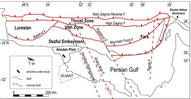
Well-log data of five exploratory wells were used to check the developed methodology. The wells are located on the axis of an anticlinal oil-field in the Abadan Plain, SW Iran (Figure 1-6). The subsurface data are limited to the Sarvak Formation. Summary of available data and specifications of some well-logs are provided in Table 1-3 and 1-4, respectively.
Table 1-2. Specifications of the ideal-logs to generate the synthetic logs.
Case Well-log Description Lower bed Thin-bed or fracture Upper bed Bed thickness (cm) Vertical resolution (cm)
1 GR (API) There is a peak at the horizon of the thin-bed. 20 50 30 30 61 2 GR (API) Deepening (finning) upward 20 100 120 30 61 3 RHOB (g.cm-3) There is a trough at the horizon of the thin-bed. 2.8 2.4 2.6 15 76 4 NPHI (%) Increasing upward 5 10 15 30 76 5 NPHI (%) There is a peak at the horizon of the thin-bed. 5 15 10 30 76
6 DT (µs.m-1) A single fracture with a dip of 60°, aperture of 1 mm, filled up with oil (281 µs/m), within a carbonate formation.
160 281 160 0.1 61
7 DT (µs.m-1) A 1 cm horizontal fractured zone (50% fractured) with a DT of 220 µs/m, within
23
Figure 1-6. Location of the field under study within the Abadan Plain, SW Iran. Modified after Sherkati and Letouzey (2004) and Rajabi et al.(2010).
Table 1-3. Available data within the Sarvak interval. #: number. GR: gamma ray, CGR: gamma ray of potassium, DT: sonic transfer time, NPHI: neutron porosity, RHOB: bulk density, DRHO: density correction, LLD: deep laterolog, LLS: shallow laterolog, MSFL: microspherically focused log, PEF: photoelectric effect.
W1 W2 W3 W4 W5 W6 Well-logs Calliper GR CGR DT NPHI RHOB DRHO LLD LLS MSFL PEF Core tests # of plugs 2 8 5 4 6 0 # of helium porosity records 38 41 416 228 258 0 # of gas permeability records 38 41 418 228 250 0 # of grain density records 0 34 0 244 258 0 # of irreducible water records 0 0 3 0 9 0 Well tests 6 3 6 3 0 2