Publisher’s version / Version de l'éditeur:
Journal of Ocean Technology, 5, 3, 2010-07-01
READ THESE TERMS AND CONDITIONS CAREFULLY BEFORE USING THIS WEBSITE.
https://nrc-publications.canada.ca/eng/copyright
Vous avez des questions? Nous pouvons vous aider. Pour communiquer directement avec un auteur, consultez la
première page de la revue dans laquelle son article a été publié afin de trouver ses coordonnées. Si vous n’arrivez pas à les repérer, communiquez avec nous à PublicationsArchive-ArchivesPublications@nrc-cnrc.gc.ca.
Questions? Contact the NRC Publications Archive team at
PublicationsArchive-ArchivesPublications@nrc-cnrc.gc.ca. If you wish to email the authors directly, please see the first page of the publication for their contact information.
NRC Publications Archive
Archives des publications du CNRC
This publication could be one of several versions: author’s original, accepted manuscript or the publisher’s version. / La version de cette publication peut être l’une des suivantes : la version prépublication de l’auteur, la version acceptée du manuscrit ou la version de l’éditeur.
Access and use of this website and the material on it are subject to the Terms and Conditions set forth at
A Hydrodynamic Basis for Estimating the Endurance of Autonomous
Underwater Vehicles for Mission Planning
Williams, C. D.
https://publications-cnrc.canada.ca/fra/droits
L’accès à ce site Web et l’utilisation de son contenu sont assujettis aux conditions présentées dans le site LISEZ CES CONDITIONS ATTENTIVEMENT AVANT D’UTILISER CE SITE WEB.
NRC Publications Record / Notice d'Archives des publications de CNRC: https://nrc-publications.canada.ca/eng/view/object/?id=682e957b-ff80-4744-a036-b3d87538c701 https://publications-cnrc.canada.ca/fra/voir/objet/?id=682e957b-ff80-4744-a036-b3d87538c701
A Hydrodynamic Basis for Estimating the Endurance of Autonomous Underwater
Vehicles for Mission Planning
Christopher D.Williams, PhD, P.Eng. Senior Research Engineer
National Research Council Canada, Institute for Ocean Technology St. John’s, Newfoundland, Canada, A1B 3T5
and
Adjunct Professor
Memorial University of Newfoundland, Faculty of Engineering and Applied Science St. John’s, Newfoundland, Canada, A1B 3X5
1
Abstract
This article presents a method for estimating the endurance of an underwater vehicle, for a typical mission scenario. The calculations are based on recent measurements in a towing tank for a new configuration for an autonomous underwater vehicle (AUV). The energy consumed by the overall system is examined for (i) straight-ahead travel in calm water and in an opposing ocean current, (ii) hovering in place in the presence of a lateral current, and, (iii) vertical descent and ascent under various ballast conditions. The cumulative energy consumption is predicted while the vehicle performs several sample missions. The results show how the mission endurance is constrained by the regime of ocean currents encountered.
2
Introduction
One of the tasks when designing a new AUV is to be able to estimate the endurance of the vehicle, for specified operating scenarios. These estimates are based on the amount of electrical power which would be consumed by all the sub-systems within the vehicle during various types of operations. For simplicity, the power consumption is divided into two parts, (a) the power consumed by the propulsion system, and, (b) the power consumed by all other components, hereinafter referred to as the ‘hotel load’ (HL). The results of these calculations are used to estimate the mass and volume for a suitable energy source, be it a battery, fuel cell or internal combustion device. Estimates of the volume and mass for a suitable energy source are required at an early stage in the design process since this volume and mass are usually a major contributor to the total vehicle size and weight.
An assumption in this article is that initial design of the vehicle has been completed and that the vehicle has the appropriate size and buoyancy characteristics to contain an energy source of sufficient capacity for the ‘required’ mission, such as the missions used in the following examples. It is the purpose of this article to show how various combinations of (i) transiting from the launch site to the survey site, (ii) descending using some appropriate technique, (iii) surveying a prescribed area (perhaps a straight line or lawn-mower pattern or station-keeping for recording images at or near a specific location), (iv) ascending, and, (v) returning to the recovery location, are affected by the choice of vehicle speed and opposing ocean currents.
3
Vehicle capabilities
The examples used in this article are for a twin pod configuration (such as that originally developed by re-searchers at the Woods Hole Oceanographic Institution) and equipped with a novel propulsion and control system developed by NRC-IOT and Marport Deep Sea Technologies Inc. The basic configuration of this
(a) forward and reverse thrust (b) lateral thrust
(c) upward thrust (d) downward thrust
(e) thrust vectors
Figure 1: Possible thruster orientations for various directions of travel for the GSC-100
autonomous underwater vehicle (AUV) is shown in Figure 1. For simplicity only the bare twin hulls and twin articulated rudder-thruster systems are shown. For the purposes of this article, the example AUV shown in Figure 1 uses the concept of the “SQX-type drive system” but otherwise does not represent any real vehicle or its performance; for simplicity we refer to this example AUV as the ‘GSC-100’.
Figure 1 shows how the twin thrusters can be oriented for the vehicle to be able to travel in certain directions. With the thrusters oriented as in (a), the vehicle travels straight-ahead or astern. With the thrusters oriented as in (b), the AUV can travel sideways, or, it can hover in-place in the presence of a lateral cross-current. In fact both rudder-thruster units have full 360◦ yaw orientation. With the
thrusters oriented as in (c), the AUV can travel vertically upward, or, hover in-place in the presence of a vertical down-current. Similarly in (d) the AUV can thrust itself vertically downward, or, can maintain station in the presence of a vertical up-welling. In the present design both thrusters are limited to ±30◦
pitch movement, as indicated in (c) and (d). Information about the real “SQX-type” vehicle and its novel propulsion and control system can be found in [1], [3] and [8]. The concept for the overall propulsion system was reported in [5]. The details of the propeller performance for a vehicle of this type were reported in [2] and [6]. The formulation for hydrodynamic simulations is presented in [7] and [9].
Table 1: Proportionality factors for various forces for the full-scale GSC-100; force coefficients are non-dimensionalized by the square of the overall length
Quantity Expression k-value Coefficient Rudder angle Resistance ku·u
2
9.24 N per (m/s)2
0.0073 0
Sway force kv·v2 422 N per (m/s)2 0.330 0
Sway force kv·v 2 278 N per (m/s)2 0.220 90 Heave force kw·w 2 148 N per (m/s)2 0.117 0
Tow-tank tests in the 200-metre towing tank in October 2009 at NRC-IOT [4] with a 0.88-scale model included (i) straight-ahead resistance tests, (ii) pure yaw tests in range -50◦ to +180◦, (iii) pure pitch tests
sway tests were the rudders tested in the two orientations of zero and 90◦. Three orthogonal forces and
the corresponding moments were measured using a six-component balance which was mounted internal to the model. The resulting full-scale force parameters are given in Table 1 for the surge, sway and heave directions. The complete formulations of the variation of the measured loads with yaw and pitch are given in [7] and [9]. For the GSC-100, Table 1 provides the results of measurements of the vehicle ‘resistance’ when towed at steady speed. The non-dimensional force coefficients which appear in Table 1 are consistent with the values in the formulations in [7] and [9]. The dimensions for the various components of this AUV are given in Table 2; Table 3 provides the full-scale values for the area, volume and mass parameters for this AUV. For the areas in Table 3, both rudders are at zero deflection, that is, their chord-lines are aligned with the longitudinal axis of the vehicle. In Table 1 the sway force coefficients are given for two cases, with both rudders at zero deflection and both at 90◦; the sway force with the rudders undeflected is about 50%
higher than when the rudders are deflected 90◦.
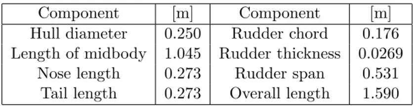
Table 2: Dimensions of various components for the full-scale GSC-100 Component [m] Component [m]
Hull diameter 0.250 Rudder chord 0.176 Length of midbody 1.045 Rudder thickness 0.0269
Nose length 0.273 Rudder span 0.531 Tail length 0.273 Overall length 1.590
Table 3: Areas, volume and mass for the full-scale GSC-100 Quantity
End view, projected area for forward travel 0.1125 m2
Side view, projected area for sway motion 0.923 m2
Plan view, projected area for heave motion 0.368 m2
Wetted surface area 2.742 m2
Displaced volume 0.140 m3
Mass when neutrally-buoyant 140 kg
The surge curve in Figure 2 shows the amount of thrust which is required to travel at various forward speeds when travelling straight ahead in calm water. Alternatively this curve shows what thrust is re-quired to hover in-place in the presence of counter-currents which are approaching from straight ahead. The maximum forward speed-over-ground (or speed of the counter-current) is, of course, limited by the amount of thrust which the twin thrusters can produce when they are oriented as in Figure 1(a). Since the amount of thrust required depends on the hydrodynamic loads which are exerted on the vehicle, which, themselves are dependent on the shape of the vehicle and the attitude of the thrusters, such thrust is independent of whether the payload sensors are powered-on or not, thus unlike in subsequent figures where there is a separate curve for each hotel load, here there is only a single “resistance” curve for all values of the hotel load.
In addition the sway curve in Figure 2 shows the amount of thrust required for the vehicle to (i) travel sideways in calm water, or, (ii) hover in-place in the presence of a lateral cross-current, when the twin thrusters are oriented as in Figure 1(b). These values of the sway force correspond to the case when both rudders are at zero deflection.
Finally the heave curve in Figure 2 shows the amount of thrust required for the vehicle to (i) travel vertically in calm water, or, (ii) hover in-place in the presence of a vertical cross-current, when the twin thrusters are oriented as in Figure 1(c) or (d).
0 0.5 1 1.5 2 2.5 3 3.5 0 20 40 60 80 100 120 140 160 180
Forward speed or speed of cross−current [m/s]
Surge, sway and heave forces [N]
Surge k = 9.24 Sway k = 278 Heave k = 148 k is for f orce = kV2
Figure 2: Force required vs vehicle relative speed for the GSC-100; see Table 1
4
Analysis for forward speed
In general the duration of a voyage for any forward speed V can be determined as follows. First the available battery energy (ABE) is equated to product of the total power consumed and the duration of the voyage. Here the total power consumed is the sum of the hotel load (HL) and the power consumed by the propulsion system. The theoretical power consumed by the propulsion system is equal to the product of the thrust required (the hydrodynamic resistance) and the forward speed. The actual power consumed by the propulsion system is equal to the ratio of the theoretical power consumed by the propulsion system to η the overall propulsive efficiency for the vehicle. Thus
Duration = ABE · η ku·V3+ HL · η
(1) where ku·V
2
is the force due to hydrodynamic resistance as given in Table 1. A plot of this function in Fig-ure 3 shows that it is similar to the right-hand side of a bell-shaped curve with a horizontal tangent at zero V , a steep slope in the region of the inflection point, and a flat portion for speeds V greater than say 3 m/s. Once the duration at a particular forward speed V is known, the range is then given by
Range = V · Duration (2)
and this result is shown in Figure 4.
In order to find the value of the vehicle speed Vopt which produces the maximum range, a derivation
provides the following result
V3 opt=
η · HL 2 · ku
(3) and the corresponding values of the maximum range appear at the maxima in the range curves in Figure 4; these values are tabulated in Table 4. Equation 3 shows that Vopt depends on all three of the ABE, the
0 1 2 3 4 5 0 5 10 15 20 25 30 35 40 45 50 Forward speed [m/s] Duration [hour] ABE is 2400 Watt.hour, η is 0.50 HL 50 W HL 100 W HL 150 W HL 200 W
Figure 3: Duration vs vehicle relative forward speed for the GSC-100
propulsive efficiency and the vehicle drag characteristics (the vehicle hydrodynamic resistance). For the special case of the vehicle travelling at speed Vopt we find that the corresponding duration is
Duration(Vopt) =
2 3·
ABE
HL (4)
which depends on neither the propulsive efficiency nor the vehicle drag characteristics. If the hotel load
0 1 2 3 4 5 0 20 40 60 80 100 120 140 Forward speed [m/s] Range [km] ABE is 2400 Watt.hour, η is 0.50 HL 50 W HL 100 W HL 150 W HL 200 W
Figure 4: Range vs vehicle relative forward speed for the GSC-100
duration occurs when the vehicle propulsion system is turned ‘off’ and all the ABE is consumed by the hotel load; for this condition
max(Duration) = ABE
HL (5)
The Range(Vopt) is given by
Range(Vopt) =
2 3·
ABE
HL ·Vopt (6)
Thus knowing the values of the four parameters k, η , HL and ABE, the graphs for range and duration can be prepared and the values of Duration(Vopt) and Range(Vopt) can be tabulated.
Based on the resistance characteristics given in Table 1, Figure 4 shows the range (distance) which could be obtained by this vehicle when advancing at a constant speed in calm water. With an available battery energy (ABE) of 2.4 kWh, a hotel load (HL) of 50 W, and, an overall propulsive efficiency η of 50 percent, the uppermost curve shows that the maximum range will be 127 km at a forward speed of 1.11 m/s; that is, the batteries will be completely depleted after travelling 127 km at this speed, and there will be no remaining energy available to either propel the vehicle, or, to energize any of the sensors. If the vehicle travels forward at a speed less than 1.11 m/s, it will be able to travel for a longer time but proportionally more energy will be consumed by the hotel load during that voyage with the result that the AUV will travel less than 127 km. If the vehicle travels at a speed which is greater than 1.11 m/s, proportionally more energy will be consumed by the propulsion system, the AUV will be able to travel for a shorter time, and the distance travelled will be less than 127 km.
When the hotel load is increased to 100 W (and other conditions remain the same), Figure 4 shows that the maximum range is reduced to about 80 km if the AUV travels at a constant forward speed of about 1.39 m/s. If the hotel load is increased to 150 W (and other conditions remain the same), the maximum range is reduced to about 61 km if the AUV travels at a constant forward speed of about 1.60 m/s. Finally, if the hotel load is increased to 200 W (and other conditions remain the same), the maximum range is reduced to about 51 km if the AUV travels at a constant forward speed of about 1.76 m/s. The four speeds 1.11, 1.39, 1.60 and 1.76 m/s are the speeds at which the four range vs speed curves attain their maximum values, that is, these are the speeds at which the range is maximal, thus these four speeds are known as the ‘optimal’ speeds for each hotel load, denoted here as Vopt.
Table 4: Parameters for the full-scale GSC-100 for optimal speed, range and duration Range Duration Maximum
HL V(opt) at V(opt) at V(opt) Duration [W] [m/s] [km] [hour] [hour]
50 1.106 127.4 32 48
100 1.39 80.3 16 24
150 1.60 61.3 10.7 16
200 1.76 50.6 8 12
The range and duration under ‘optimal’ conditions of forward travel in calm water are summarized from Figure 4 in Table 4.
The range values from Figure 4 suggest that missions of length 50 km should be possible with 2.4 kWh of ABE, if forward speeds near these ‘optimal’ values are used. Typically the transit and return phases will be accomplished using a hotel load of 50 W when the inertial navigation system, CTD (conductivity, temperature and depth sensors), altimeter, DVL (Doppler velocity log) etc. are energized. During the survey phase the hotel load may increase to typically 100, 150 or 200 W depending on which additional sensors are energized e.g. side-scan sonar, multi-beam sonar, camera and lights, acoustic modem, acoustic
tracking system etc. Such combinations of energy usage will show the portions of the mission which will consume the most energy and thus will be the limiting factors for real missions, and, which portions are negligible in comparison to the total energy consumed during the mission.
Figure 3 shows the duration of each voyage corresponding to the same operating conditions as in Figure 4, for the same range of forward speeds as in Figure 4. Clearly the duration of the voyage is largest when the forward speed of the vehicle is zero and all the ABE is consumed by the hotel load. But this may not be a practical mission! Thus the curves in Figures 3 and 4 show how the mission planner must trade-off (i) the distance which must be travelled (the track length which much be surveyed) with (ii) the number of sensors which can be switched ‘on’ during the survey, and, (iii) with the speed of travel of the AUV. An alternative interpretation of Figure 3 is that it shows how long the AUV can hover in place (perform station-keeping) in the presence of a constant counter-current. Each curve indicates that the stronger is the counter-current, the less time the AUV can retain its position in space. For example, for a counter-current speed of 1 m/s, with 2.4 kWh of ABE, the AUV can hold station for about 35 hours when the HL is 50 W, for about 20 hours when the HL is 100 W, for about 14 hours when the HL is 150 W, and, for about 11 hours when the HL is 200 W. The maximum counter-current which the AUV can withstand is of course limited by the maximum thrust which the propulsion system (the twin thrusters) can produce when thrusting in the forward direction. For a DC electric-motor drive system, the maximum thrust may be limited by any of the following factors: (i) design of the propeller, (ii) continuous (or short-term) power output of the thruster motor, (iii) maximum electrical current capacity of the motor-speed controller, or, (iv) maximum electrical current capacity of the energy source.
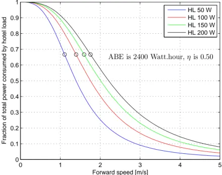
0 1 2 3 4 5 0 0.1 0.2 0.3 0.4 0.5 0.6 0.7 0.8 0.9 1 Forward speed [m/s]
Fraction of total power consumed by hotel load
ABE is 2400 Watt.hour, η is 0.50
HL 50 W HL 100 W HL 150 W HL 200 W
Figure 5: Fraction of total power consumed by hotel load vs vehicle relative forward speed for the GSC-100
Figure 5 shows the ratio (fraction) of the HL to the total load (total power consumed) for various forward speeds. On the left all four curves converge to the same point where, at zero forward speed, all the power consumed is that due to the HL. To the right, at higher forward speeds, this ratio decreases as more and more power is consumed by the propulsion system, in relation to the HL. Note that for the four optimal speeds from Figure 4 (1.11, 1.39, 1.60 and 1.76 m/s), it appears that the ratio of HL to the total power is
about 0.67; this observation will be discussed later in Appendix A.
5
Analysis for lateral (sway) movement
0.1 0.2 0.3 0.4 0.5 0.6 0.7 0.8 0.9 1 10 15 20 25 30 35 40 45 50
Cross−current flow speed [m/s]
Duration [hour] Sway force = 278 v2 ABE is 2400 Watt.hour, η is 0.50 HL 50 W HL 100 W HL 150 W HL 200 W
Figure 6: Duration vs vehicle relative sway speed for the GSC-100
Figure 1(b) shows how the thrusters should be oriented for (i) travelling sideways in calm water, or, for (ii) hovering in place (station-keeping) in the presence of a constant lateral cross-current. For station-keeping (or hovering in place) in a cross-current, the concept of ‘optimal speed’ does not apply so the duration expression given above in equation (1) is the only one which is useful. In general the duration for hovering in any lateral cross-current of speed ‘v’ is given by
Duration = ABE · η kv·v3+ HL · η
(7) Again the maximum duration would be for the case of zero cross-current; for any non-zero cross-current the duration will be less than the maximum value. The curve of Duration vs ‘v’ should have a similar shape to that in Figure 3. From Table 1 where kv is 278 for this case, Figure 6 can be prepared. All
four curves in Figure 6 indicate that the stronger is the lateral cross-current, the less time the AUV can retain its position (hover in-place). The maximum lateral cross-current which the AUV can withstand is of course limited by the maximum thrust which the propulsion system can produce when thrusting in the lateral direction.
When the AUV is hovering in a cross-current, there is no analogue for the ‘optimal speed’ which was observed in Figures 3 and 4, so no graph of range vs speed of the cross-current is shown while hovering in-place. And, the concept of ‘range’ as distance travelled does not apply when the AUV is hovering in-place.
6
Analysis for vertical (heave) movement
Figures 1(c) and 1(d) show how the thrusters should be oriented for (i) travelling vertically in calm water, or, for (ii) hovering in place (station-keeping) in the presence of a constant vertical cross-current. In general
the duration for hovering in any vertical cross-current speed ‘w’ is given by Duration = ABE · η
kw·w3+ HL · η
(8) Again the maximum duration would be for the case of zero vertical current; for any non-zero cross-current the duration will be less that the maximum value. The curve of Duration vs ‘w’ should have a similar shape to that in Figure 3. From Table 1 where kw is 148 for this case, Figure 7 can be prepared.
0.1 0.2 0.3 0.4 0.5 0.6 0.7 0.8 0.9 1 10 15 20 25 30 35 40 45 50
Vertical−current flow speed [m/s]
Duration [hour] Heave force = 148 w2 ABE is 2400 Watt.hour, η is 0.50 HL 50 W HL 100 W HL 150 W HL 200 W
Figure 7: Duration vs vehicle relative heave speed for the GSC-100
Figure 7 is similar to Figure 6 except that Figure 7 shows how long the AUV can hover in place (perform station-keeping) in the presence of a constant vertical cross-current, either upward or downward. Again, all four curves in Figure 7 indicate that the stronger is the vertical cross-current, the less time AUV can retain its position (hover in-place). The maximum vertical cross-current which the AUV can withstand is of course limited by the maximum thrust which the propulsion system can produce when the thrusters are pitched to their maximum angle of ±30◦; in this orientation the maximum vertical thrust is about half the
maximum thrust which can be produced for counter-acting either head currents or lateral currents.
7
Analysis for descent and ascent
There are a variety of mechanisms which can be used to enable an AUV to descend and ascend. A variable buoyancy system (VBS) of fore and aft tanks can be used both to alter overall net buoyancy and to provide pitch trim adjustments. While suitable for large submarines, such a mechanism is not usually employed in small AUVs where a VBS would consume valuable payload space, is expensive and adds complexity to vehicle. Thus a simpler device such as external ‘descent weight’ can be used; here a lump mass is suspended from a light-weight chain which hangs below the vehicle; once the mass reaches the seabed, if the weight of the chain has been chosen to balance the net positive upward buoyant force (NPUBF), then the vehicle will remain a constant distance (the chain length) above the seabed.
A simple device for free ascent is the ‘drop weight’. Here the vehicle is equipped with a small weight which is attached with a release hook inside the lower portion of the hull; for ascent the latch is opened and the
‘drop weight’ is released. The following analysis considers the use of both a ‘descent weight’ and a ‘drop weight’.
For operational reasons it is often desirable to have the AUV traverse near surface as far as possible toward the survey site in order to have the most-recent GPS position available so as to minimize posi-tion errors due to a lengthy deduced-reckoning segment of the survey. Similarly it may be desirable to have the AUV traverse near surface as far as possible in order to have an active RF connection with the launch site or mother ship in case there is a change in mission required since departure. In reality many AUVs are programmed to use a spiral trajectory during descent. Thus the following example missions are simplified but they portray the salient features of how to estimate the energy consumption. Simple mis-sion calculations can be refined further if required; the following three mismis-sions are for illustrative purposes. If the vehicle is equipped with a ‘descent weight’ for the purpose of descending without the use of the propulsion system, the hydrodynamic properties from Table 1 can be used to determine the ‘terminal velocity’ of descent. Once the terminal velocity is known, the time to descend is then simply the ratio of the depth to the terminal velocity. When falling at a constant speed ‘w’ due to an additional descent weight ‘∇’, the total upward force is BF + kw·w2 where ‘BF’ is the buoyant force, and, the total downward
force is W+∇. So if the buoyant force (due to the displaced volume of the vehicle) and the weight of the vehicle W are essentially the same (as is the case when the vehicle is neutrally ballasted) and ‘∇’ is the net weight (in water) which is producing the descent, then
w =√(∇/kw) (9)
gives the terminal velocity. Typically an AUV is ballasted, before launch, with about one percent of its mass acting upward (e.g. the MUN Explorer AUV has a mass of about 800 kg so is ballasted upward at 8 kg) so we use one percent in the calculations which follow. For the GSC-100 with a mass of 140 kg (Table 3) if ‘∇’ is 148 N (about 15 kg) then ∇/kw= 1 so the rate of descent ‘w’ for this vehicle is 1.0 m/s downward.
The case of aided ascent with an inflatable buoyancy bag or ‘drop weight’ is similar to the above for descent. The upward terminal velocity will be
w =√(NP UBF/kw) (10)
where ‘NPUBF’ is the net positive upward buoyant force due to the lifting bag. Again if ‘NPUBF’ is 148 N (about 15 kg) then the rate of ascent ‘w’ for this vehicle is 1.0 m/s upward.
From the value in Table 1 for kw for the heave direction, one can derive the results shown in Figure 8.
This figure shows the terminal velocity for descent which can be achieved for various values of the descent weight. The vehicle starts near the ocean surface from a condition of neutral buoyancy with a mass of 140 kg; the descent weight is added (without a change in displaced volume) such that the vehicle will descend toward the seabed. For each additional weight there is different terminal velocity which is computed from an equality of the descent weight and the upward hydrodynamic (heave) force as given in Figure 2 by kww
2
with a value of kw of 148 N/(m/s) 2
. For example, for a descent weight of 30 N the descent rate is 0.45 m/s.
Similarly Figure 8 can be used to determine the terminal velocity for ascent for various values of net posi-tive upward buoyant force (NPUBF). For example this figure shows that if drop weight of 30 N is released (without a change in displaced volume) then the ascent rate will be 0.45 m/s.
Figure 9 shows the time to descend 500 m when various values for the descent weight are used. Similarly the same curve shows the time to ascend 500 m when an equivalent amount of NPUBF is used. These times vary from 45 minutes when a 5 N weight is used to less than 15 minutes when a 50 N weight is used.
0 10 20 30 40 50 0.2 0.25 0.3 0.35 0.4 0.45 0.5 0.55 0.6 0.65
Descent weight or net upward buoyant force [N]
Terminal velocity for descent or ascent [m/s]
Displaced volume is 0.140 m3
Mass when neutrally buoyant is 140 kg
Figure 8: Terminal velocities for descent and ascent for the GSC-100
0 10 20 30 40 50 10 15 20 25 30 35 40 45 50
Descent weight or net upward buoyant force [N]
Time to descend or ascend [min]
Displaced volume is 0.140 m3
Mass when neutrally buoyant is 140 kg
Figure 9: Time to descend and ascend for the GSC-100
7.1 Energy cost associated with descent using a descent weight
Here it is assumed that the vehicle starts near the ocean surface from a condition of neutral buoyancy thus the descent weight will cause the vehicle to free-fall toward the seabed. For each additional weight there is a different terminal velocity ‘w’ which is computed from an equality of the descent weight and the upward hydrodynamic (heave) force. Since no propulsive power is required, the power consumed is only that due to the hotel load during descent. The time to descend in free-fall due to the descent weight is given by Figure 9 so the energy consumed during descent is simply the product of the time to descend and the HL.
7.2 Energy cost associated with the descent of a neutrally-buoyant vehicle while using propulsion
Here it is assumed that the vehicle starts near the ocean surface from a condition of neutral buoyancy and that the propulsion system will be required to drive the vehicle toward the seabed at some desired rate ‘w’. The thrust required from the propulsion system will be given by kw·w
2
and the theoretical propulsion power required will be given by kw·w
3
and the actual propulsion power required (APPR) by kw·w 3
/η. The time to descend at the propelled speed ‘w’ is given by the ratio of the distance to the seabed ‘d’ to ‘w’ so the energy consumed during descent is simply the product of the time to descend and the sum (HL + APPR).
7.3 Energy cost associated with the descent of a positively-buoyant vehicle while using propulsion
Here it is assumed that the vehicle starts near the ocean surface from a condition of net positive upward buoyancy and that the propulsion system will be required to drive the vehicle toward the seabed at some desired rate ‘w’. The thrust required from the propulsion system to descend will be given by
kw·w 2
+ N P U BF (11)
and the theoretical propulsion power required to descend will be given by (kw·w
2
+ N P U BF ) · w (12)
Again the time ‘t’ to descend at the propelled speed ‘w’ is given by the ratio of the distance to the seabed to ‘w’ so the energy consumed during this mode of descent is simply
∆E = [HL · η + kw·w 3
+ w · N P U BF ] · t (13) 7.4 Energy cost associated with ascent using a drop weight
Here it is assumed that the vehicle starts near the seabed from a condition of neutral buoyancy thus the releasing of the drop weight will cause the vehicle to rise freely toward the ocean surface. For any particular value of the drop weight, there is different terminal velocity ‘w’ which is computed from an equality of the upward net buoyant force weight and the downward hydrodynamic (heave) force. Since no propulsive power is required, the power consumed is only that due to the hotel load during ascent. The time to ascend freely due to the drop weight is given by Figure 9 so the energy consumed during ascent is simply the product of the time to ascend and the HL.
7.5 Energy cost associated with the ascent of a neutrally-buoyant vehicle while using propulsion
Here it is assumed that the vehicle starts near the seabed from a condition of neutral buoyancy and that the propulsion system will be required to drive the vehicle toward the ocean surface at some desired rate ‘w’. The thrust required from the propulsion system will be given by kw·w
2
and the theoretical propulsion power required will be given by kw·w
3
and the actual propulsion power required (APPR) by kw·w 3
/η. The time to ascend at the propelled speed ‘w’ is given by the ratio of the distance from the seabed to the ocean surface ‘d’ to ‘w’ so the energy consumed during ascent is simply the product of the time to descend and the sum (HL + APPR).
7.6 Energy cost associated with the ascent of a positively-buoyant vehicle while using propulsion
Here it is assumed that the vehicle starts near the seabed from a condition of net positive upward buoyancy and that the propulsion system will be required to drive the vehicle toward the seabed at some desired rate ‘w’ which is in excess of the speed at which the vehicle would rise freely due to buoyancy alone. The thrust required from the propulsion system to ascend will be given by
kw·w 2
−N P U BF (14)
which is less than the thrust required to descend, and the theoretical propulsion power required to ascend will be given by
(kw·w 2
−N P U BF ) · w (15)
Again the time ‘t’ to ascend at the propelled speed ‘w’ is given by the ratio of the distance from the seabed to the ocean surface ‘d’ to ‘w’ so the energy consumed during this mode of ascent is simply
∆E = [HL · η + kw·w 3
−w · N P U BF ] · t (16)
8
Analysis for thruster requirements
The following analysis is concerned with establishing the thruster propulsion requirements for travelling along a straight line on the seabed in the presence of a cross-current. Whereas for a traditional surface ship or AUV with a non-azimuthing thruster, the vessel is required to use an off-track heading when attempt-ing to make forward progress in the presence of a lateral cross-current. For many types of sensors (e.g. downward-looking sonar) it is a requirement that the axis of the sensor remain aligned with the specified survey line on the seabed. Thus the vectored-thrust capability of the GSC-100 AUV make it an ideal platform for such surveys.
The hydrodynamic forces and moments which act on an AUV (such as the GSC-100) while it is moving in surge at a certain speed, and, while simultaneously experiencing a cross-flow of a certain speed in the sway direction, will depend in a complicated way on the angle with which the effective flow vector is ap-proaching the vehicle. Considering the wake structure alone, there will be a wake created by each of the hull sections, plus a wake from each of the rudders, elevators, thruster bodies and propellers. Thus the actual flow field in which the propellers must operate will not be a simple superposition of the wake due to a pure surge flow and a wake due to a pure cross-flow. In this paper, for the purposes of performing a first-order energy-consumption calculation, such complications are ignored.
In reality the vehicle controllers will use the real-time measurements from the on-board sensors (inertial motion measurement unit, Doppler velocity log, compass etc.) to vary the instantaneous yaw and pitch orientation and RPM of each thruster, to adjust the vehicle heading and speed in order to ensure that the vehicle executes a straight-line track relative to the seabed. Clearly such complications must be considered when designing the heading and speed controllers.
For simplicity we take the desired direction of travel to be northward and the direction of the cross-current to be from west to east. By using the respective k-values from Table 1 in conjunction with the surge (northward) and lateral (west-to-east) speeds, the magnitude and direction of the required thrust vector can be determined. These thrust-vector direction values can then be used to determine the yaw angle of the thruster with respect to the longitudinal centreline of the vehicle; see Figure 1(e). When the cross-current is stronger than the forward speed, the thruster angle approaches 90◦, and the thrust vector points to the
0 0.5 1 1.5 2 0 10 20 30 40 50 60 70 80
Vehicle northward speed [m/s]
Thrust magnitude [N] West−to−east cross−current 0.1 to 0.5 m/s v = 0.1 m/s v = 0.2 m/s v = 0.3 m/s v = 0.4 m/s v = 0.5 m/s
Figure 10: Magnitude of the total thrust vector required for northward travel in the presence of a lateral cross-current for the GSC-100
track (when projected onto the seabed) should be straight north.
The magnitude and direction of the required thrust vector were computed for various northward vehicle speeds and west-to-east cross-current speeds. These results are shown in Figures 10 and 11.
Figure 10 shows the magnitude of the total thrust vector for five different magnitudes of the lateral (west-to-east) cross-current, from 0.1 to 0.5 m/s, for a range of northward (forward) vehicle speeds from 0.1 to 2.0 m/s. When the vehicle northward speed is low, the thrust required is dominated by the speed of the cross-current. Note that in all cases it is the speed of the cross-current which dominates the thrust, not the forward speed since the value of kv for the sway force is 278 N/(m/s)
2
and the value of kw for the surge
force is 9.24 N/(m/s)2
.
Figure 11 shows the thruster yaw angle, with respect to the longitudinal centreline of the vehicle, for the same conditions as in Figure 10. Only for the lowest cross-current and highest northward vehicle speeds does this yaw angle reduce to less than 10◦. As summarized in Table 5, for the case of a 0.5 m/s lateral
cross-current, each thruster is required to produce half of the total Tu and half of the total Tv and thus
half of the total magnitude of the required thrust vector; note that the direction of each thrust vector is the same for both thrusters, unless differential thrust is used to counteract an undesirable hydrodynamic yaw moment. The values which are summarized in Table 5 appear again in §11 for example mission C.
9
Example Mission A
From the above graphs for the thruster requirements we can estimate the amount of battery energy which will be consumed for various types of missions. As an example we propose the following example mission, Mission A. The AUV is to transit 10 km from the launch location to the work site at shallow depth, descend to a depth of 500 m by using a 4 kg mass as a descent weight, travel at that depth for a distance of 50 km, return to the surface by using a 1.4 kg mass as a drop weight, and, return 15 km to the recovery location.
0 0.5 1 1.5 2 0 10 20 30 40 50 60 70 80 90
Vehicle northward speed [m/s]
Thruster yaw angle [deg] from straight ahead
West−to−east cross−current 0.1 to 0.5 m/s v = 0.1 m/s v = 0.2 m/s v = 0.3 m/s v = 0.4 m/s v = 0.5 m/s
Figure 11: Direction of the total thrust vector required for northward travel in the presence of a lateral cross-current for the GSC-100
Table 5: Magnitude and direction of the total thrust vector for various forward speed and cross-current combinations; see Figure 1(e)
Forward Cross- Thrust Thrust
speed Thrust current Thrust vector vector u Tu v Tv magnitude direction [m/s] [N] [m/s] [N] [N] [deg] 1.106 11.3 0.5 69.5 70.4 80.8 1.39 17.9 0.5 69.5 71.8 75.6 1.60 23.7 0.5 69.5 73.4 71.2 1.76 28.6 0.5 69.5 75.2 67.6
Here it is assumed that the survey phase will be executed at the ‘optimal speed’ for the specified hotel load. With a descent weight of mass 4 kg, the descent rate is 0.52 m/s; for a drop weight of mass 1.4 kg, the ascent rate is 0.30 m/s.
Figure 12 shows the cumulative amount of energy consumed as the mission proceeds in terms of the energy consumed vs elapsed time within the mission. Figure 12 contains three curves, one for each of the hotel loads 100, 150 and 200 W. Recall that each of those hotel loads has a different ‘optimal speed‘, thus the time taken to survey the 50 km track will vary with the hotel load. The lower curve, for a HL of 100 W, falls below the dashed line at 2.4 kWh, thus this mission can be accomplished within the available battery energy. The middle curve, for a HL of 150 W, rises above the 2.4 kWh line only during the return to the recovery site; instead of being able to complete the return distance of 15 km, the AUV can probably complete only 11 km of the return journey. When the HL required for surveying is 200 W, the upper curve shows that the AUV will be unable to complete the survey phase with an ABE of 2.4 kWh and will thus be unable to complete the mission. This type of diagram shows quickly what types of missions are feasible in calm water with a given ABE which spends all its time travelling straight ahead, for the various hotel loads required.
0 5 10 15 20 0 500 1000 1500 2000 2500 3000
Cumulative time [hour]
Cumulative energy consumed [Watt.hour]
Transit 10 km at u(opt) of 1.106 m/s Descend 500 m with 4 kg at 0.52 m/s Survey 50 km at 1.39, 1.60 & 1.76 m/s Ascend 500 m with 1.4 kg buoyancy at 0.3 m/s Return 15 km at u(opt) of 1.106 m/s Mission A
Survey HL 100 W Survey HL 150 W Survey HL 200 W
Figure 12: Mission A: using optimal forward speeds for surveys with the GSC-100
Table 6: Parameters for Mission A for the GSC-100
Distance HL Speed Thrust Time APP HL+APP ∆(Energy) Phase [km] [W] [m/s] [N] [hour] [W] [W] [W.h] Transit 10 50 1.106 11.3 2.51 25.0 75.0 188.4 Descent 0.5 50 0.52 0 0.27 0.0 50.0 13.4 Survey 50 100 1.39 17.9 9.99 49.6 149.6 1495 Survey 50 150 1.60 23.7 8.68 75.7 225.7 1959 Survey 50 200 1.76 28.6 7.89 100.7 300.7 2373 Ascent 0.5 50 0.30 0 0.46 0.0 50.0 23.1 Return 15 50 1.106 11.3 3.77 25.0 75.0 282.6
Total energy consumed with survey HL of 100 W 2003 Total energy consumed with survey HL of 150 W 2467 Total energy consumed with survey HL of 200 W 2881
Table 6 summarizes, for Mission A, the distance travelled, the hotel load, the speed of travel, the thrust required, the time taken, the propulsion power required, and the amount of energy consumed, for each of the five phases, for the case of calm water.
The three curves in Figure 12 show that an ABE of at least 2.9 kWh would be required for successful completion of all three surveys which require up to 200 W of hotel load during the survey phase. If a maximum of only 150 W of hotel load is required during the survey phase then about 2.5 kWh of ABE would be sufficient.
0 5 10 15 0 500 1000 1500 2000 2500 3000 3500
Cumulative time [hour]
Cumulative energy consumed [Watt.hour]
Transit 10 km at 1.5 m/s Descend 500 m NB thrust at 0.52 m/s Survey 50 km at 1.75, 2.0 & 2.2 m/s Ascend 500 m NB thrust at 0.3 m/s Return 15 km at 1.5 m/s Mission B Survey HL 100 W Survey HL 150 W Survey HL 200 W
Figure 13: Mission B: using higher-than-optimal forward speeds for transits and surveys with the GSC-100
10
Example Mission B
Mission B is similar to Mission A in terms of distances travelled but the transit and survey and return speeds all exceed the ‘optimal speeds’. Also the descent and ascent phases are different; in Mission B the vehicle is assumed to be neutrally-buoyant and no descent weight is available for descent (and no drop weight is available for ascent) thus the AUV is require to use its propulsion system for ascent and descent. Thus the energy consumed in Mission B for the same distances travelled will be greater than the energy consumed in Mission A. The purpose of Mission B is to see how sensitive are the energies consumed to travelling at the ‘optimal speeds’.
In Mission B the transit speed is 1.5 m/s, the descent is 500 m with a neutrally-buoyant vehicle which is propelled downward at a rate of 0.52 m/s. The survey speeds with hotel loads of 100, 150 and 200 W are 1.75, 2.00 and 2.20 m/s. The ascent is 500 m with a neutrally-buoyant vehicle which is propelled upward at a rate of 0.30 m/s. The return speed is 1.5 m/s over a distance of 15 km.
Figure 13 shows the cumulative amount of energy consumed as the mission proceeds, as energy vs elapsed time, for Mission B. The lower curve, for a HL of 100 W, falls below the dashed line at 2.4 kWh, thus this mission can be accomplished within the available battery energy. The middle curve, for a HL of 150 W, rises above the 2.4 kWh line during the return to the recovery site; instead of being able to complete the return distance of 15 km, the AUV can probably complete only 2 km of the return journey. When the HL required for surveying is 200 W, the upper curve shows that the AUV will be able to complete only about 43 km of the intended 50 km of the survey phase with an ABE of 2.4 kWh and will thus be unable to complete the mission.
This type of diagram shows quickly what types of missions are feasible in calm water with a given ABE which spends all its time travelling straight ahead, for the various hotel loads required, and, what amount of ABE would be required if the vehicle is to be able to complete the desired survey when hotel loads of 150 W and 200 W are required, depending on the type of survey-sensor used.
Table 7: Parameters for Mission B for the GSC-100
Distance HL Speed Thrust Time APP HL+APP ∆(Energy) Phase [km] [W] [m/s] [N] [hour] [W] [W] [W.h] Transit 10 50 1.5 20.8 1.85 62.4 112.4 208 Descent 0.5 50 0.52 40.0 0.27 41.6 91.6 24.5 Survey 50 100 1.75 28.3 7.94 99.0 199.0 1580 Survey 50 150 2.00 37.0 6.94 147.8 297.8 2068 Survey 50 200 2.20 44.7 6.31 196.8 396.8 2505 Ascent 0.5 50 0.30 13.3 0.46 8.0 58.0 26.8 Return 15 50 1.5 20.8 2.78 62.4 112.4 312 Total energy consumed with survey HL of 100 W 2151 Total energy consumed with survey HL of 150 W 2640 Total energy consumed with survey HL of 200 W 3076
Table 7 summarizes, for Mission B, the distance travelled, the hotel load, the speed of travel, the thrust required, the time taken, the propulsion power required, and the amount of energy consumed, for each of the five phases, for the case of calm water. Notice that the energy consumed during the 200 W survey phase alone is 2505 Wh, thus that survey phase alone exceeds the ABE of 2.4 kWh.
In comparing Mission B with Mission A, recall that in Mission A the AUV uses (i) a descent weight (which it releases once it reaches the 500 m depth at which depth the AUV was trimmed to be neutrally buoyant), and, (b) releases a drop-weight for ascent. The amount of energy consumed in Mission A will be less than in Mission B but there is a trade-off in complexity of requiring (i) a releasable descent weight, and, (ii) a releasable drop-weight for ascent.
The three curves in Figure 13 show that an ABE of at least 3.2 kWh would be required for successful completion of all three surveys which involve using higher-than-optimal transit and survey speeds, and active propulsion to descend and ascend.
11
Example Mission C
Mission C uses the same distance, speed and hotel load conditions as Mission A except that the vehicle now encounters an west-to-east cross-current of speed 0.5 m/s as it attempts to travel northward and southward along a lawn-mower-type survey track. Again as in §8 the survey track lines and vehicle path, when projected onto the seabed, will run either straight north or south. In Mission C the transit speed is the value of Vopt for a HL of 50 W thus 1.11 m/s over a distance of 10 km. The descent is 500 m with a
neutrally-buoyant vehicle which uses a descent weight of mass 4 kg so the rate of descent is 0.52 m/s. The survey speeds with hotel loads of 100, 150 and 200 W are at the Vopt values of 1.39, 1.60 and 1.76m/s.
The ascent is 500 m with a neutrally-buoyant vehicle which jetisons a drop weight of mass 1.4 kg so the rate of ascent is 0.30 m/s. The return speed is the value of Vopt for a HL of 50 W thus 1.11 m/s over a
distance of 15 km.
Figure 14 shows the cumulative amount of energy consumed as the mission proceeds, as energy vs elapsed time, for Mission C. The lower curve, for a HL of 100 W, rises above the 2.4 kWh line during the survey phase; instead of being able to complete the survey distance of 50 km, the AUV can probably complete only 36 km of tis distance. The middle curve, for a HL of 150 W, rises above the 2.4 kWh line during the survey phase; instead of being able to complete the survey distance of 50 km, the AUV can probably complete only 33 km of this distance. When the HL required for surveying is 200 W, the upper curve shows that the AUV will be able to complete only about 30 km of the intended 50 km of the survey phase
Table 8: Parameters for Mission C for the GSC-100
Speed Thrust Current Thrust Thrust HL+ ∆ Distance HL u Tu v Tv mag Time APP APP Energy
Phase [km] [W] [m/s] [N] [m/s] [N] [N] [hour] [W] [W] [W.h] Transit 10 50 1.106 11.3 0 0 11.3 2.5 25.0 75.0 188 Descent 0.5 50 0.52 0 0 0 0 0.27 0 50.0 13.4 Survey 50 100 1.39 17.9 0.5 69.5 71.8 10.0 200 300 2992 Survey 50 150 1.60 23.7 0.5 69.5 73.4 8.7 235 385 3341 Survey 50 200 1.76 28.6 0.5 69.5 75.2 7.9 265 465 3666 Ascent 0.5 50 0.30 0 0 0 0 0.46 0 50.0 23.1 Return 15 50 1.106 11.3 0 0 11.3 3.8 25.0 75.0 283 Total energy consumed with survey HL of 100 W 3500 Total energy consumed with survey HL of 150 W 3849 Total energy consumed with survey HL of 200 W 4174
with an ABE of 2.4 kWh and will thus be unable to complete the mission.
0 5 10 15 20 0 500 1000 1500 2000 2500 3000 3500 4000 4500
Cumulative time [hour]
Cumulative energy consumed [Watt.hour]
Transit 10 km at u(opt) of 1.106 m/s Descend 500 m with 4 kg at 0.52 m/s Survey 50 km at 1.39, 1.60 & 1.76 m/s with sideways crab current 0.5 m/s Ascend 500 m with 1.4 kg buoyancy at 0.3 m/s Return 15 km at u(opt) 1.106 m/s Mission C
Survey HL 100 W Survey HL 150 W Survey HL 200 W
Figure 14: Mission C: using optimal forward speeds for surveys with vectored thrust to com-pensate for a 0.5 m/s lateral cross-currents near the seabed with the GSC-100
Table 8 summarizes, for Mission C, the distance travelled, the hotel load, the vehicle and cross-current speeds, the thrust required, the time taken, the propulsion power required, and the amount of energy consumed, for each of the five phases, for the case of a 0.5 m/s cross-current during the survey phase and in calm water otherwise. Column 5 contains values of the component of thrust required to maintain the speed-over-ground (SOG) of 1.39 m/s in the northward direction; column 7 contains values of the component of thrust required to counteract the west-to-east current so that the SOG in the west-to-east direction is zero. Notice that the energy consumed during all three survey phases exceeds the ABE of 2.4 kWh.
The major differences in energy consumption appear during the survey phases, as expected. For straight-ahead travel in calm water, as in Mission A, at the ‘optimal’ speeds, the energies consumed during the
survey phases were (see Table 6) 1495, 1959 and 2373 Wh for hotel loads of 100, 150 and 200 W respectively. Mission C used the same values of ‘optimal’ speeds of 1.39, 1.60 and 1.76 m/s for the northward SOG. In Mission C (see Table 8) the corresponding survey values were 2992, 3341 and 3666 Wh. Thus the effect of a 0.5 m/s cross-current has caused the energy consumption (at the same vehicle speed in each case) to rise by 1497, 1382 and 1293 Wh respectively, or in percentage terms by 100, 71 and 55 percent, respectively, over that in Mission A. These values show that the effect of a cross-current can have a significant effect on the operational and design factors for such an AUV.
The three curves in Figure 14 show that an ABE of at least 4.2 kWh would be required for successful completion of all three surveys in the presence of a constant cross-path current of 0.5 m/s, which is not unusual in ocean surveys.
12
Discussion
Comparing Mission B to Mission A emphasizes the importance of travelling at Vopt. Mission C shows that
with 2.4 kWh the vehicle could survey in conditions with lateral cross-currents for a period of perhaps up to six hours so the length of the survey leg must be reduced from 50 km to 30 km. The three energy consumption curves for Mission C show that an ABE of at least 4.2 kWh would be required for successful completion of all three surveys in the presence of a constant cross-path current of 0.5 m/s, which is not unusual in ocean surveys.
Diagrams such as the cumulative energy consumption plots of Figures 12, 13 and 14 quickly show the designer how trade-offs in propulsion load (vehicle speed), HL and survey distance affect the required ABE. It can be concluded from the three simple mission scenarios that the descent or ascent portions of Fig-ures 12, 13 and 14 are not significant contributions to the total energy consumed during a composite voyage. For example in Tables 6, 7 and 8 that (i) the energy consumed during descent never exceeds 1.1 percent of the total, andm (ii) the energy consumed during ascent never exceeds 1.2 percent of the total. Comparing the values in Table 7 with those in Table 6, in the survey portions of Mission B the forward speeds were increased by 25 percent over those in Mission A, which used the optimal speeds. The result is that in Mission B, 95 percent more power is consumed by the propulsion system, as expected, since this power (APPR) is proportional to the cube of the forward speed. However the total energy consumed only increased by seven percent and the total time required to complete the voyage decreased by 22 percent. So from a time-to-complete perspective, there appears to be an advantage in travelling at speeds greater than the optimal speed for that HL, since the HL accounts for two-thirds of the total power consumed while the APPR accounts for one-third of the total power consumed. Figure 5 shows that by increasing the survey speed by 25 percent above the optimal speed, the fraction is now 50-50.
The initial ‘resistance’ experiments with the 0.88-scale model were completed in October 2009 in the NRC-IOT 200 m towing tank and the results from those experiments formed the basis for this article. Full-scale manoeuvring experiments with an SQX-500 vehicle were performed in the 22 by 8 by 4 metre Flume Tank at the Marine Institute in December 2009; these included roll and pitch damping experiments in calm water. Since then the propeller open-water experiments were completed in the NRC-IOT Cavitation Tunnel in March 2010, and, thruster open-water experiments in the MUN water channel were completed in April 2010. Full-vehicle self-propulsion and energy-consumption experiments were conducted in the Flume Tank at the Marine Institute in May 2010. Bench-top experiments with a thrust and torque dynamometer to measure the mechanical efficiency of the propulsion system, including the friction losses due to the shaft bearings and O-ring seals, were completed in August 2010. The purpose of these measurements is to quantify the overall propulsion efficiency for the various types of manoeuvres, thus validating the estimates
for power consumption which have been made in this article.
13
Summary
As a result of a set of simple towing tank tests to determine the hydrodynamic resistance for (i) forward travel, (ii) lateral travel (movements), and, (iii) vertical movements, we can estimate the amount of energy required to execute various types of missions. The examples shown are for a twin-hull, twin-vectored-thruster vehicle which is capable of forward, lateral and vertical travel in calm water, and, is capable of hovering in-place in the presence of lateral or vertical ocean currents. The three example missions illuminate the essential features of a simple, first-order method, which is intended for the preliminary as-sessment of energy system requirements for various potential survey lengths and optimal survey speeds. The examples show the relative contributions of the various portions of a typical voyage to the total and cumulative energy consumption, by the hotel load and propulsion loads. Although these examples use a simple experimentally-obtained model to characterize the hydrodynamic performance of the AUV, al-ternative models could be based on analytical, semi-empirical or CFD or other methods. Because this method is first-order, it assumes steady-state conditions during each portion (segment) of the voyage, thus no unsteady phenomena such as abrupt manoeuvres or effects of ocean surface waves are included. The set of calculations and results which are presented in this article are unique since no other free-swimming AUV can travel forward (or in reverse), hover (station-keeping) and ascend (or descend) using a single multi-function propulsion system.
14
Acknowledgements
The author thanks the staff and students at NRC-IOT and Marport Deep Sea Technologies Inc. for their on-going support and encouragement for the experiments which provided the data which lead to the ideas presented in this article. In particular thanks go to Dr. Moqin He of NRC-IOT, to Neil Riggs, David Shea, Peter Crocker and Michael Snow of Marport Deep Sea Technologies Inc., and, to Dr. Ralf Bachmayer of Memorial University. Thanks go to the reviewers for their insight and suggestions which have been used to clarify several points made in this article.
15
References
Although some of the reports below contain commercially-sensitive information, the essential results re-quired for this article have been made available, with the kind permission of Marport Deep Sea Technologies Inc, and have been published in the open literature.
1. David Shea, Neil Riggs, Ralf Bachmayer, Christopher D. Williams, “Prototype Development of the SQX-1 Autonomous Underwater Vehicle”, proceedings of the IEEE-MTS OCEANS’09 conference, Bre-men, Germany, 11 to 14 May 2009.
2. Moqin He and Christopher D. Williams, “Propeller Design and Power Performance Estimation for SQX-1”, NRC-IOT report TR-2009-11, June 2009. Protected.
3. David Shea, Neil Riggs, Ralf Bachmayer and Christopher D. Williams, “Preliminary Testing of the SQX-1 Autonomous Underwater Vehicle”, proceedings of the 16th International Symposium on Unmanned Untethered Submersible Technology (UUST’09), Durham, NH, 23 to 26 August 2009.
4. Moqin He, Christopher D. Williams, Brad Butt and Andrew Clarke, “Hydrodynamic Model Tests for Marport Vehicle SQX-500”, NRC-IOT report TR-2009-29, October 2009. Protected.
5. Andrew Clarke, “Propulsion System of the SQX-500 UUV”, NRC-IOT report SR-2009-26, December 2009. Protected.
6. Moqin He, Christopher D. Williams, Thomas House and Darrell Sparkes, “Propeller Testing and Power Estimation for the Marport Vehicle SQX-500”, NRC-IOT report TR-2010-08, April 2010. Protected. 7. Moqin He and Christopher D. Williams, “A Simple Method for Hydrodynamic Prediction of the Ma-noeuvring Performance of a Twin-Pod Vehicle”, proceedings of the 29th American Towing Tank Conference (ATTC), Annapolis, Maryland, USA, 11 to 13 August 2010.
8. David Shea, Christopher D. Williams, Moqin He, Peter Crocker, Neil Riggs and Ralf Bachmayer, “De-sign and Testing of the Marport SQX-500 Twin-Pod AUV”, proceedings of the IEEE AUV 2010 conference, Monterey, CA, USA, 01 to 03 September 2010.
9. Moqin He, Christopher D. Williams, Peter Crocker, David Shea, Neil Riggs and Ralf Bachmayer, “A Simulator Developed for a Twin-Pod AUV, The Marport SQX-500”, accepted for presentation at the 9th International Conference on Hydrodynamics, 11 to 15 October 2010, Shanghai, China.
Appendix A. Derivation of the 1/3 and 2/3 rules of thumb for the power
consumed by an AUV travelling at the optimal forward speed
It was shown in Figure 5 at the end of §4 that when a self-propelled vehicle travels at the ‘optimal’ speed (the forward speed at which the maximum range is obtained when surveying with a given hotel load) that the ratio of that hotel load (HL) to the total power consumed is about 2/3; this can now formally be shown to be true.
To prove the above assertion let the hydrodynamic resistance be expressed as
Resistance = k · V2 (17)
and let the total power consumed (TPC) be expressed as
T P C = HL + AP P (18)
where the amount of actual propulsion power required (APPR) can be calculated from the theoretical propulsion power (TPP)
T P P = V · Resistance = k · V3 (19) by including the overall propulsive efficiency η as follows
AP P R = T P P/η (20)
Recall from equation 3 that the ‘optimal’ forward speed Vopt for each hotel load is given by
V3 opt=
η · HL
2 · k (21)
thus the theoretical propulsion power consumed when travelling at forward speed Vopt is
T P P (Vopt) = k · V 3 opt= k · ( η · HL 2 · k ) = 1 2 ·η · HL (22)
The actual propulsion power consumed when travelling at forward speed Vopt is then given by
AP P R(Vopt) =
T P P (Vopt)
η =
1
2·HL (23)
hence the total power consumed when travelling at forward speed Vopt is given by
T P C(Vopt) = HL + AP P R(Vopt) = HL +
1
2 ·HL = 3
2·HL (24)
thus we find that
HL = 2
3 ·T P C(Vopt) (25)
which can be used in expression (23) to show that AP P R(Vopt) =
1
2·HL = 1
3 ·T P C(Vopt) (26)
Again the maximum range, the range at speed Vopt, is given by
Range(Vopt) =
2 3·
ABE
and the mission duration at speed Vopt is given by Duration(Vopt) = 2 3· ABE HL (28)
Thus one concludes from equation (25) that when the vehicle is travelling forward at the constant ‘optimal’ speed Vopt, the hotel load accounts for two-thirds of the total power consumed, and, from equation (26) one
concludes that the actual propulsion power consumed accounts for one-third of the total power consumed. Inherent in this derivation are two assumptions (i) that the the coefficient ‘k’ for the hydrodynamic re-sistance is a constant, thus independent of Reynolds Number, and, (ii) the overall propulsive efficiency η is independent of forward speed. If these assumptions do not hold, a similar calculation procedure can be invoked to estimate correctly the energy consumed at each forward speed. In any case the above ‘1/3 and 2/3’ rules of thumb can provide useful initial estimates of (i) what will be the ‘optimal’ forward speed (for a particular hotel load) which will provide the maximum mission range, (ii) the total power and total energy required, and, (iii) the likely duration of travel at that ‘optimal’ speed.
For example, if the customer specifies a particular hotel load (HL), and if you have for your vehicle reasonable estimates for ‘k’ and η, then expression (21) gives a first estimate of the ‘optimal’ forward speed for that HL. Then expression (26) or (23) provides a first estimate of the actual propulsion power consumed when travelling at that forward speed, and, expression (24) provides a first estimate of the total power consumed when travelling at that forward speed. The likely maximum range which could be obtained from a battery pack of available energy ABE can then be obtained using expression (27). Finally the likely mission duration (hours) which could be obtained from that ABE when travelling at that forward speed can be obtained using expression (28). If that value of Vopt is satisfactory but either (i) the duration at
speed Vopt is not sufficient, or, (ii) the range at speed Vopt is insufficient, then since the expressions (28)
and (27) show that the duration at speed Vopt and the range at speed Vopt are each proportional to the
ABE, then either the expression
ABE2 = ABE1· Duration2 Duration1 (29) or the expression ABE2 = ABE1· Range2 Range1 (30) can be used to estimate the required amount of ABE.
The above calculations are simple to perform, and, will likely provide estimates which are within a few percent of estimates made using a more exact or complicated formulation. Practical experience with these simple estimates and real vehicles will establish the validity and usefulness of the above ‘1/3 and 2/3’ rules of thumb for the power consumed by an AUV travelling at the optimal forward speed.