Activation of conductive pathways via deformation-induced instabilities

Activation of Conductive Pathways via

Deformation-induced Instabilities

by

MASSACHUSETTS INSTITUTE

Xinchen Ni

OF TECHNOLOCY

AUG 15 2014

B.S.

Mechanical Engineering

LIBRARIES

Fudan University, Shanghai, China 2012

Submitted to the Department of Mechanical Engineering

in partial fulfillment of the requirements for the degrees of

Master of Science in Mechanical Engineering

at the

Massachusetts Institute of Technology

June 2014

C Massachusetts Institute of Technology. All Rights Reserved

Signature redacted

A uthor...

Department of Mechanical Engineering May 13, 2014

Signature redacted

Certified by...

Mary C. Boyce Ford Professr echanical Engineering

Signature redacted

A ccepted by...

David E. Hardt Ralph E. and Eloise F. Cross Professor of Mechanical Engineering

Activation of Conductive Pathways via

Deformation-induced Instabilities

by

Xinchen Ni

Submitted to the Department of Mechanical Engineering

on May 13, 2014, in partial fulfillment of the

requirements for the degree of

Master of Science in Mechanical Engineering

Abstract

Inspired by the pattern transformation of periodic elastomeric cellular structures, the purpose of this work is to exploit this unique ability to activate conductive via

deformation-induced instabilities. Two microstructural features, the contact nub and the conductive pathway, are introduced to make connections within the void and between the voids upon pattern

transformation. Finite element-based micromechanical models are employed to investigate the effects of the contact nub geometries, conductive pathway patterns and elastic properties of the coating and substrate materials on the buckling responses of the structure. Finally, a flexible circuit that can be switched on and off by an applied uniaxial load is fabricated based on the finite element analysis and demonstrated the ability to activate conductive pathways in response to an external triggering stimulus.

Thesis Supervisor: Mary C. Boyce

Acknowlidgements

First and foremost, I would like to express my deepest appreciation to my adviser,

Professor Mary C. Boyce. To think upon where I started from two years ago, and how far I have come since then, I feel extremely grateful to have you as my mentor. Your patience, kindness and knowledge have helped me to develop into the person I am now. I wish you all the best at your new future at Columbia University and I will always be proud of being your student.

I would also like to thank everyone in the Boyce's lab. Thank you, Stephan for your guidance along the way. Thank you, Hansohl for all the coffee break and late night chats. Thank you, Narges for treating me as your little brother. Thank you, Mark for always being funny and positive. Thank you, Erica for all the tutoring on Zwick. Thank you, Shabnam and Swati for always being patient and answering my questions. I also like to thank Juliette, Leslie, Joan and Una for making administrative matter much easier.

Above all, I would like to thank my friends and family for all your love and support. Thank you, Ke, for being with me and supporting me through all the ups and downs. I am so grateful to have you and I promise that I will do the same thing to you. Thank you, Mom and Dad. There are really no words to describe how grateful I am and how much I love you. I know you have scarified so much to help me to get to where I am right now. Yes, your son has got a degree from MIT and he will keep working hard to realize his dream. But I want to tell you that no matter where I am and no matter what I do, my love is always with you.

Table of Contents

Chapter 1 Introduction ... ... 1

1.1 Overview of periodic elastomeric structures and their applications ... 1

1.2 Thesis objective... 4

Chapter 2 Background ... 7

2.1 List of symbols... 7

2.2 Characterization of material behavior... 8

2.3 Boundary conditions for infinite periodic structures... 10

2.4 Eigen analysis... 12

2.5 Post-buckling analysis... 13

2.6 References ... 14

Chapter 3 Pattern transformation of periodic elastomeric structures with a square array of circular holes ... 15

3.1 Infinite periodic structure, unit cell and RVE ... 15

3.2 Analysis of instability... 17

3.3 Post-buckling analysis... 19

3.4 Understanding the effect of void-volume fraction... 20

3.5 Conclusions ... 24

3.6 References ... 25

Chapter 4 Micromechanical model based design of contact nubs...26

4.1 Conceptual design ... 26

4.2 Design parameters... 27

4.4 Effect of void-volume fractions for fixed nub geometries... 32

4.5 Design of contact nubs for circular holes on a hexagonal lattice... 34

4.6 References ... 36

Chapter

5

Micromechanical model based design of conductive pathways...37

5.1 Modeling rationale for thin film bonded to an elastomer substrate ... 37

5.2 Three dim ensional periodic structures ... 39

5.3 Design of conductive pathways... 41

5.4 Discussion on the design of conductive pathways... 49

5.5 References ... 51

Chapter 6 Experim ents... 53

6.1 Substrate fabrication... 53

6.2 Conductive pathways printing... 55

6.3 Experim ents and results ... 58

6.4 References ... 62

Chapter 7 Conclusion and future w ork ... 63

7.1 Conclusions... 63

List of Figures

Figure 1 .1 (a) Image of an opal bracelet, a natural photonic crystal (Taken from Wikipedia) (b) Demonstration of a photonic band gap [1] (c) Phononic band gaps for a 2D periodic structures with a square array of circular holes at different strains (Taken from Bertoldi and Boyce 2008 [4]) Figure 1.2 Images of the progressive deformation of an elastomeric matrix comprising a square array of circular holes (Taken from Overvelde, Shan et al. 2012 [10])

Figure 1.3 Sequence of progressively deformed shapes of a "Buckliball," a spherical elastomeric shell patterned with a regular array of circular voids, due to the decrease of internal pressure (Taken from Shim, Perdigou et al. 2012 [13])

Figure 2.1 (a) Acrylic mold (b) Cylindrical testing specimen with a radius of 10 mm and a height of 6.35 mm (c) Uniaxial compression test setup

Figure 2.2 Engineering stress vs. principle stretch. Comparison between experiment and Neo-Hookean model

Figure 2.3 A periodic structure and its corresponding unit cell and RVE

Figure 2.4 A RVE deforming under periodic boundary conditions with pi and P2 periodically located on the RVE boundary

Figure 3.1 (a) An infinite periodic structure with circular holes (b) Corresponding unit cell (c) Corresponding 2 x 2 RVE (d) Corresponding 3 x 3 RVE (e) Corresponding 4 x 4 RVE Figure 3.2 Infinite periodic structures and their corresponding unit cells with void-volume fraction $ = 30%, 50% and 60%

Figure 3.3 First and second eigenmode for

4

= 50% for p = (2,2), p = (3,3), p = (4,4), p = (5,5) and p = (6,6)

Figure 3.4 Eigenvalue vs. RVE size for

4=

50%. $' = 30% and

4'

= 60% showed similar trends with different eigenvalues.

Figure 3.6 (a) A beam subject to compressive load (b) The first buckling mode of the beam when the load reaches a critical value.

Figure 3.7 Dimensions of the beam

Figure 3.8 (a) Inter-void ligament slenderness of RVE with different void volume fractions (b) relation between critical stress of the ligament and the macroscopic critical stress

Figure 3.9 normalized acr-ligament vs. d/1

Figure 4.1 The conceptual design of contact nubs Figure 4.2 Nub design parameters

Figure 4.3 Nub shapes with B = 0.5R: 0.1R: 0.7R, and C = 0.9R: 0.1R: 1.1R while keeping A = 0.25R fixed

Figure 4.4 First mode of the specimen with Nub shapes with A = 0.25R, B = 0.5R, C = 0.6R

Figure 4.5 Eigenvalues vs. B for different values of C for a fixed A=0.25R

Figure 4.6 Nub shapes with C=0.9R, R, 1.IR, and A=0.15R, 0.25R, 0.75R, while keep B=0.7R fixed

Figure 4.7 eigenvalues vs A for different values of C

Figure 4.8 The 2D unit cell with qj = 20%, 50%, 70%. Nub design parameters are A =

0.25R, B = 0.5R, C = 0.9R.

Figure 4.9 Comparison of eigenvalues between structures with and without nubs

Figure 4.10 Two elastomeric porous structures with different hole arrangements buckle under uniaxial compression (Taken from Shim, Shan et al. 2013 [2])

Figure 4.11 (a) a finite-sized sample with a 7 x 8 hexagonal array of circular holes with nubs; (b) a RVE representing its infinite periodic counterpart.

Figure 5.1 (a) A film stretches with the substrate when well bonded to the substrate. (b) A film wrinkles under compressive load when well bonded to the substrate. (Taken from Li, Suo et al. 2005[1]) (c) A film detaches from the substrate and ruptures under tensile load. (d) A film detaches from the substrate under compressive load. (Taken from Huang, et al. 2012) Figure 5.2 Specimen dimensions

Figure 5.3 First four eigenmodes and eigenvalues of the 2D structure (plane strain) and the same structure with different thicknesses t/R (t = 1/8, 1/4, 1/2, 5/4)

Figure 5.4 Nominal strain vs. nominal stress for 2D structure and 3D structures with thickness t/R = 1/8 and t/R = 1/4

Figure 5.5 Transformative patterned elastomeric materials in undeformed and deformed states Figure 5.6 Potential conductive pathways on the deformed patterned structure

Figure 5.7 a 2 x 2 RVE with nubs and thin film coating to realize the conductive pathway depicted in Figure 5.6(a)

Figure 5.8 First buckling mode and eigenvalue of Specimen 1,2,3 and 2D strucutre (from left to right)

Figure 5.9 First buckling mode and eigenvalue of Specimen 4, 5 and 6 (from left to right) Figure 5.10 First buckling mode and eigenvalue of Specimen 7, 8 and 9 (from left to right) Figure 5.11 Nominal strain vs. nominal stress for specimen 3 and 7

Figure 5.12 Strain levels within the film

Figure 5.13 RVEs with conductive line width d/R = 1/40, d/R = 3/40 and d/R = 3/20

Figure 5.14 Specimen 3 with conductive line width d/R = 1/40, d/R = 3/40 and d/R = 3/20

Figure 5.15 Specimen 7 with conductive line width d/R = 1/40, d/R = 3/40 and d/R = 3/20

Figure 6.1 (a) Acrylic base with microstructures made by laser cutter. (b) Pillars made using 3D printer were inserted into the base.

Figure 6.2 (a) Final substrate (b) Zoomed-in image of the RVE with four unit cells (top view) (c) Zoomed-in image of one circular void with four contact nubs (top view)

Figure 6.3 (a) 3D printer (b) printed conductive lines and nozzle (c) a printed circuit (Taken from Russo, Ahn et al. 2011 [4])

Figure 6.4 Schematics of designed conductive pathways (a) disconnected circuit in an undeformed configuration (b) connected circuit in a deformed configuration

Figure 6.5 Printing setup

Figure 6.6 Printed conductive pathways

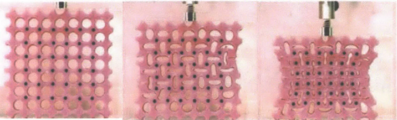
Figure 6.7 Experimental and numerical images of the specimen at different strains

Figure 6.8 Nominal stress vs. nominal strain curve showing experimental and numerical results Figure 6.9 Demonstration circuit layout

Figure 6.10 Images of progressive deformation of the demonstration circuit. (a) undeformed circuit; conductive pathways disconnected (b) deforming circuit (c) deformed circuit; conductive pathways connected to light up the LED

Chapter 1

Introduction

Periodic microstructures abound in nature and demonstrate numerous interesting and unique mechanical, photonic and hydrophobic properties.

In recent years, a number of research groups have focused on periodic elastomeric

structures because of their unique ability to switch between two very different configurations due to instability in response to an external triggering stimulus. These structures offer exciting

opportunities to design lightweight responsive and reconfigurable devices that have a wide range of applications in sensors, bioengineering, microfluidics and photonics. For example, photonic switches could be created to filter waves if the periodic pattern length scales are in the order of the wavelength of light.

In this chapter, an overview of state-of-the-art research on periodic elastomeric structures is presented, and the objective of this study is proposed at the end.

1.1 Overview of periodic elastomeric structures and their applications

1.1.1 Phononic and photonic crystals

Phononic and photonic crystals are periodic structures that are capable of controlling the propagation of waves through band gaps: a range in frequency where wave propagation is barred [1]. Phononic crystals have exciting applications such as sound filters, acoustic wave guides, and vibration isolators; Photonic crystals avenues to control light waves such as tuning colors and directing light. Figure 1.1(a) shows an image of an opal bracelet. It is essentially a natural photonic crystal with periodic microstructures that give rise to its iridescent color. Figure 1.1(b) illustrates the concept of a phononic band gap. The yellow region in the picture represents a frequency range where sound wave propagation is forbidden [1].

It is desirable to design tunable photonic and phononic band gap systems because most photonic and phononic crystals only operate at a fixed frequency range. Great advances have

been made towards this goal using methods such as altering out-of-plane modes with

piezoelectric effects [2] and directly physically changing the positioning of the periodic structure [3]. The dramatic shape change of periodic patterned elastomeric structures due to instability also provides one potential alternative: to use deformation and other stimulus as an external means to control band gaps in photonic and phononic crystals [4]. Figure 1.1(c) demonstrates this idea. It shows the different band gaps of a 2D periodic elastomeric structure with a square array of circular voids at different strain levels.

C X U1 L 01i Strain-0.0 *at Strain=0.03 a ftain=0.06 a0 L x W V'3 Strain 0.1 04, L Ms* x Wga

x-y gap z gap Complete gap r

Figure 1.1 (a) Image of an opal bracelet, a natural photonic crystal (Taken from Wikipedia) (b) Demonstration of a photonic band gap [1] (c) Phononic band gaps for a 2D periodic structures with a square array of circular holes at different strains (Taken from Bertoldi and Boyce 2008 [4])

b 0.8 0.7 0.6 016 0.4 0.3 0.2 0.1 0 U

I

rsg=:Z--PhOtONC 8" Gop

I

1.1.2 Auxetic materials

Mechanical instability of periodic patterned elastomeric structures can also be used to design 3D metamaterials with switchable Poisson's ratio. The Poisson's ratio is defined as the ratio between the transverse and axial strain when subjected to uniaxial stresses [5]. When compressed, most materials expand outwards in the directions orthogonal to the applied load resulting in a positive Poisson's ratio. However, the pattern transforming material of Mullins, Boyce et al. [6] was demonstrated to have a Possion's ratio that transforms from a positive Possion's ratio to a negative Possion's ratio after the deformation-induced pattern transformation [7], [8].

Figure 1.2 shows a periodic patterned structure with a square array of circular holes. When the structure is uniaxially compressed, a structural transformation induced by instabilities occurs [8], [9] and the initial circular holes transform into elongated, almost closed ellipses, giving rise to the shrinkage of the entire structure. Moreover, a significant lateral contraction is observed and is further accentuated with the increase of applied strain. This material behavior offers great potential for designing energy absorbing devices.

Figure 1.2 Images of the progressive deformation of an elastomeric matrix comprising a square array of circular holes (Taken from Overvelde, Shan et al. 2012 [10])

1.1.3 Soft origami-like structure

The attractive characteristics of periodic elastomeric structures also provide routes for the fabrication of foldable and origami-like structures that have a wide range of applications such as drug delivery capsules [11], material synthesis agents and soft-material robots [12].

One interesting example of a 3D origami-like structure is shown in Figure 1.3. It was developed by Professor Pedro Reis's group at MIT and Professor Katia Bertoldi's group at Harvard and is based on the pattern transforming structure of Mullins et al. [6] The structure is named the "Buckliball" because the shape change is a result of local buckling of ligaments in the structure. The "Buckliball" comprises a spherical elastomeric shell patterned with 24 carefully spaced dimples. The inner pressure is controlled by a motorized syringe pump. When air is sucked out of the ball, the thin ligaments between the dimples buckle, inducing a "cooperative buckling cascade" of the skeleton of the ball in the same manner as the planar cases of Mullins et al. [6], [13]. As a result, the circular dimples turn into ellipses that are almost closed and the ball volume is reduced by up to 54%. Moreover, the structure remains spherical throughout the process. Figure 1.3 shows the progressive images of the deformation.

A big advantage of the buckling-induced folding mechanism of the elastomeric structures is that it is fully reversible and can be achieved without moving parts. This opens the possibility for reversible encapsulation over a wide range of length scales.

Figure 1.3 Sequence of progressively deformed shapes of a "Buckliball," a spherical elastomeric shell patterned with a regular array of circular voids, due to the decrease of internal pressure (Taken from Shim, Perdigou et al. 2012 [13])

1.2 Thesis objective

Great advances have been made to take advantage of the reversible and dramatic pattern transformation of periodic elastomeric structures, such as the tunable phononic crystals and the Buckliball for encapsulation. Moreover, while there have been extensive works on the effect of topology on the behaviors of periodic elastomeric structures [7], [10], [14], [15] as well as the

stretchability of thin films on elastomeric substrates [16], [17], little has been investigated on the overall buckling and postbuckling behavior of the elastomer when it is periodically patterned with another material.

In this thesis, a flexible circuit with switchable conductive pathways that can be

controlled by deformation-induced instabilities is designed based on finite element analysis. Also, 3D printed electronics techniques are exploited to fabricate a working demonstration circuit.

A major challenge of the design is to make connections between the voids of the continuous porous structure as it undertakes a dramatic shape change induced by instabilities. Here, we first introduce two novel design concepts of contact nubs and conduction pathways. We then choose an optimal geometry of those features based on finite element analysis and confirm our design with experiments. Finally, we present a robust flexible circuit harnessing the

optimized elastomeric substrate geometries that is fabricated using 3D printing techniques and stretchable conductive ink.

1.3 References

[1] J. D. Joannopoulos, S. G. Johnson, J. N. Winn, and R. D. Meade, Photonic Crystals: Molding the Flow of Light (Second Edition) (Google eBook). Princeton University Press, 2011,p.304.

[2] Z. Hou, F. Wu, and Y. Liu, "Phononic crystals containing piezoelectric material," Solid State Commun., vol. 130, no. 11, pp. 745-749, Jun. 2004.

[3] Y. Yao, Z. Hou, and Y. Liu, "The two-dimensional phononic band gaps tuned by the position of the additional rod," Phys. Lett. A, vol. 362, no. 5-6, pp. 494-499, Mar. 2007. [4] K. Bertoldi and M. C. Boyce, "Wave propagation and instabilities in monolithic and

periodically structured elastomeric materials undergoing large deformations," Phys. Rev. B, vol. 78, no. 18, 2008.

[5] G. N. Greaves, A. L. Greer, R. S. Lakes, and T. Rouxel, "Poisson's ratio and modern materials.," Nat. Mater., vol. 10, no. 11, pp. 823-3 7, Nov. 2011.

[6] T. Mullin, S. Deschanel, K. Bertoldi, and M. Boyce, "Pattern Transformation Triggered by Deformation," Phys. Rev. Lett., vol. 99, no. 8, p. 084301, Aug. 2007.

[71 S. Babaee, J. Shim, J. C. Weaver, E. R. Chen, N. Patel, and K. Bertoldi, "3D Soft Metsmaterials with Negative Poisson's Ratio," Adv. Mater., vol. 25, no. 36, pp. 5044-5049, 2013.

[8] K. Bertoldi, P. M. Reis, S. Willshaw, and T. Mullin, "Negative Poisson's Ratio Behavior Induced by an Elastic Instability," Adv. Mater., vol. 22, no. 3, p. 361-+, 2010.

[9] K. Bertoldi, M. C. Boyce, S. Deschanel, S. M. Prange, and T. Mullin, "Mechanics of deformation-triggered pattern transformations and superelastic behavior in periodic elastomeric structures," J. Mech. Phys. Solids, vol. 56, no. 8, pp. 2642-2668, 2008. [10] J. T. B. Overvelde, S. Shan, and K. Bertoldi, "Compaction through buckling in 2D

periodic, soft and porous structures: effect of pore shape.," Adv. Mater., vol. 24, no. 17, pp. 2337-42, May 2012.

[11] Y. Zhu, J. Shi, W. Shen, X. Dong, J. Feng, M. Ruan, and Y. Li, "Stimuli-responsive controlled drug release from a hollow mesoporous silica sphere/polyelectrolyte multilayer core-shell structure.," Angew. Chem. Int. Ed. Engl., vol. 44, no. 32, pp. 5083-7, Aug. 2005.

[12] C. Laschi, M. Cianchetti, B. Mazzolai, L. Margheri, M. Follador, and P. Dario, "Soft Robot Arm Inspired by the Octopus," Adv. Robot., vol. 26, no. 7, pp. 709-727, Jan. 2012. [13] J. Shim, C. Perdigou, E. R. Chen, K. Bertoldi, and P. M. Reis, "Buckling-induced

encapsulation of structured elastic shells under pressure.," Proc. Natl. Acad. Sci. U. S. A., vol. 109, no. 16, pp. 5978-83, Apr. 2012.

[14] S. H. Kang, S. Shan, W. L. Noorduin, M. Khan, J. Aizenberg, and K. Bertoldi, "Buckling-induced reversible symmetry breaking and amplification of chirality using supported cellular structures.," Adv. Mater., vol. 25, no. 24, pp. 3380-5, Jun. 2013.

[15] S. Singamaneni, K. Bertoldi, S. Chang, J.-H. Jang, S. L. Young, E. L. Thomas, M. C. Boyce, and V. V. Tsukruk, "Bifurcated Mechanical Behavior of Deformed Periodic Porous Solids," Adv. Funct. Mater., vol. 19, no. 9, pp. 1426-1436, May 2009. [16] T. Li and Z. Suo, "Deformability of thin metal films on elastomer substrates," Int. J.

Solids Struct., vol. 43, no. 7-8, pp. 2351-2363, 2006.

[17] T. Li, Z. Huang, Z. Suo, S. P. Lacour, and S. Wagner, "Stretchability of thin metal films on elastomer substrates," Appl. Phys. Lett., vol. 85, no. 16, p. 3435, Oct. 2004.

Chapter 2

Background

In this chapter, we first characterize the material behavior of the silicone rubber we use throughout the study. Then, the method of periodic boundary conditions as a means for modeling periodic structures and Refined Eigen Analysis are introduced. The former is useful for

analyzing large structures with repeating units, while the latter is a typical approach to explore the instability of structures.

2.1 List of symbols

We use standard notation of modem is listed below. X x X = X(X, _t) F = VX J = detF > 0 u = x - X H = Vu F = RU = VR U,V R C =U2 = FTF,B = V2 FFT 1 E = -(C -1) 2 Ii(B)

continuum mechanics throughout this work, which

Material point in the reference body Spatial point in the deformed body Motion function Deformation gradient Determinant of F Displacement Displacement gradient Polar decomposition of F Right and left stretch tensor Rotation tensor

Right and left Cauchy-Green tensor Green strain tensor

xi > 0 Principal stretches

il Left principal basis

{rI} Right principal basis

T Cauchy stress

TR First Piola stress

TRR Second Piola stress

Principal value of Cauchy stress/true stress Principal value of Piola stress/engineering

Si stress/nominal stress

PR Mass density per unit reference volume

IR Free energy density per unit reference volume

boR Body force per unit reference volume

p Arbitrary pressure

Generalized shear modulus

* Eigen modes

2.2 Characterization of material behavior

A silicone rubber (Elite Double 8, Zhermack) is used throughout this study. The major macroscopic physical characteristic of this material is its ability to sustain large reversible strains with negligible hysteresis, which makes it ideal to be modeled by the theory of finite elasticity. Uniaxial compression tests were conducted to determine the material constants.

A mold was made from acrylic sheets using laser cutting to cast the material testing specimen. The testing specimen was a cylinder with a radius of 10 mm and a height of 6.35 mm (Figure 2.1).

Figure 2.1 (a) Acrylic mold (b) Cylindrical testing specimen with a radius of 10 mm and a height of 6.35 mm (c) Uniaxial compression test setup

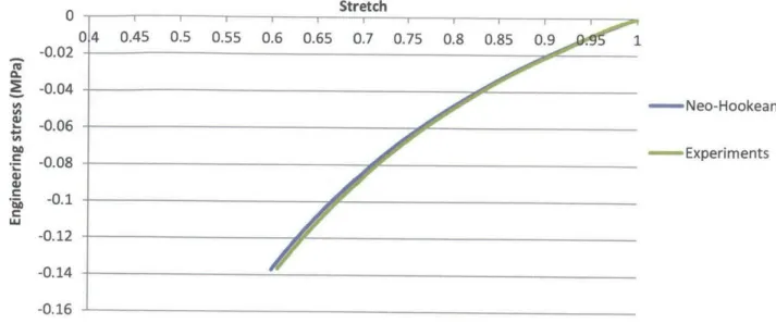
Uniaxial compression tests were conducted on the specimen to characterize the material response of the elastomeric matrix and the behavior was found to be well captured by a simple Neo-Hookean model. The specimen was subjected to uniaxial compression at different strain rate using a Zwick screw-driven testing machine. Vaseline was used to reduce the friction effects between the sample and the plates. The tests showed that the material exhibits a behavior typical for elastomers: large strain elastic behavior with negligible rate dependence and negligible hysteresis during a loading-unloading cycle. The material behavior at a compression speed of 20 mm/min is reported in Figure 2.2 and is used to determine the shear modulus.

The uniaxial stress-strain behavior of the material up to an applied strain of over 35% was found to be well captured using an incompressible Neo-Hookean model, whose strain energy is,

$= (1 1-3) (2.1)

where p.o is the initial shear modulus and I, is the first invariant of the left Cauchy Green tensor. This covers well beyond the range of strain in this study. After curve fitting, the initial shear modulus was found to be 0.058 MPa.

Stretch 0 0 4 0.45 0.5 0.55 0.6 0.65 0.7 0.75 0.8 0.85 0.9 . 1 -0.02 ----0.04 , -- _Neo-Hookean -0.06 -Experiments -0.08 -0.1 LU -0.12 -0.14 -0.16

Figure 2.2 _{Engineering stress vs. principle stretch. Comparison between experiment and}

Neo-Hookean model

2.3 Boundary conditions for infinite periodic structures

When analyzing a structure with complicated and repeating units of microstructures, we often use periodic boundary conditions. One methodology was first developed by Danielsson, Parks and Boyce [1].

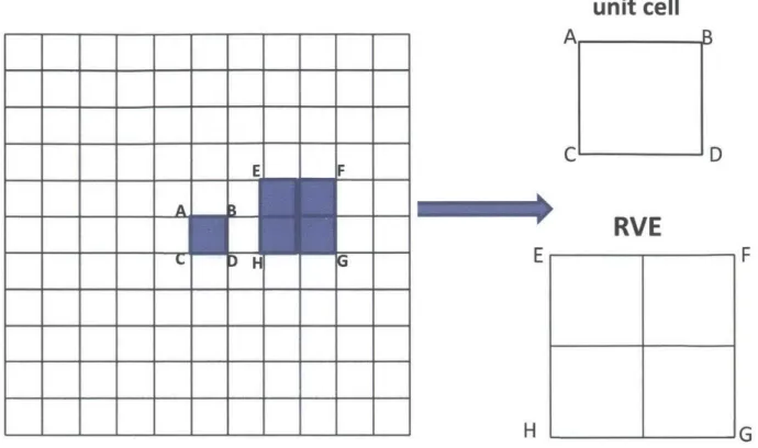
The key idea of this methodology is that instead of analyzing the entire structure, we consider a representative volume element (RVE) that contains one or multiple unit cells of the structure. A unit cell is defined as the smallest repeating geometric units. Figure 2.3 shows a structure with repeating units. Square ABCD is a unit cell; the unit cell itself is typically taken as the RVE. However, with deformation, instabilities may actually have their lowest energy mode over multiple "initial unit cells", hence changing the "unit cell" to require more of the "initial unit cells". Therefore, we also consider RVEs include multiple "initial unit cells" such as the square EFHG containing four unit cells. We impose boundary conditions on the RVE to capture the periodic nature of the deformation of the RVE edge boundaries, written in terms of the macroscopic deformation gradient and the local position of the edge nodes. Using periodic boundary conditions is not only computationally efficient but also eliminates the artificial boundary effects of the finite structure.

unit cell

A fI CD

RVE

E F E' D H - G

Figure 2.3 A periodic structure and its corresponding unit cell and RVE

Figure 2.4 A RVE deforming under periodic boundary conditions with pi and P2 periodically located on the RVE boundary

F G F E H K P2 E P1 P2 HG

P1

T

'G

The periodic boundary condition can be mathematically defined as follows:

uP2 - uP, = H(Xp2 - Xp) = (F - 1)(X 2 - Xp1) (2.2)

where pi and P2 are two points periodically located on the RVE boundary, shown in Figure 2.4. F denotes the macroscopic applied deformation gradient.

To implement in finite element programs, we impose the macroscopic deformation by prescribing the components of H through a set of virtual nodes. The components of H are assigned to be the displacement components of the virtual nodes. Therefore, by prescribing corresponding displacements of the virtual nodes, we can realize different macroscopic loading conditions including uniaxial compression, biaxial tension and simple shear. Using the principle of virtual power, the components of the macroscopic first Piola stress S are identified as the reaction forces of the virtual nodes divided by VO, the reference volume of the RVE. Then the Cauchy stress can be found through T = L SF T, where V is the volume of the deformed configuration. The components of the macroscopic nominal strain are simply equal to the displacements of the virtual nodes.

2.4 Eigen analysis

In this study, we mostly focused on infinite periodic structures for the sake of computational efficiency with a few analyses performed on finite-sized specimens to enable comparison with the experimental results.

The stability of both the finite-sized specimens and the corresponding infinite periodic structures was first examined using eigenvalue analysis. It is a linear perturbation procedure that perturbs an arbitrary reference load by X and seeks alternative configurations that can sustain the perturbed load [2], [3]. It is essentially an eigenvalue problem. In our study, this procedure was implemented using the *BUCKLE module in the commercial finite element package

ABAQUS/Standard. It returns an eigenmode which corresponds to a buckled shape and an eigenvalue which corresponds to a critical stress/strain. There can be multiple eigenvalues and eigenmodes.

It is rather straightforward for a finite-sized specimen. However for its infinite periodic counterpart a Refined Eigen Analysis [4], [5] is needed because it is possible that there exists a microscopic bifurcation with a longer periodic length than a "unit cell." A "unit cell" here is defined as the smallest repeating geometry unit. Therefore, in order to obtain the correct eigenvalue and eigenmode of an infinite periodic structure, we should perform eigenvalue analysis on RVEs with an increasing number of unit cells. Then the critical load of the infinite periodic structure is defined as the infimum of the critical load on all possible RVEs. This approach is referred to as Refined Eigen Analysis.

In particular, an RVE is constructed consisting of pY cells, where p = (Pl, P2) and Y serves as a unit cell. Periodic boundary conditions described in Section 2.2 were imposed and linear buckling analysis was performed on each RVE with increasing p. In theory, we need to examine an infinite number of RVEs for different values of p, but for practical purposes, RVE size up to 10Y by 10Y is sufficient to get a reasonable understanding of material behaviors.

2.5

Post-buckling analysis

The eigenvalue analysis using *BUCKLE in ABAQUS is a one-step linear analysis that only returns the end-state data, i.e., eigenvalues and eigenmodes. It does not provide any information about the material response prior to or after the bifurcation. On the other hand, a static analysis using *STATIC in ABAQUS does generate progressive data at each time increment, but it does not capture the bifurcation at the critical load. In order to depict both the buckling and evolution of material behavior, we introduce an imperfection in the form of the first buckling mode 41(the eigenmode with the lowest eigenvalue) obtained from the linear buckling analysis to perturb the mesh by a small amount, scaled by a scale factor w,

dx + d(2.7)

AX0 = w 2 (27

Thus, the perturbation Ax0 introduced into the mesh is a fraction of the average center-to-center distance between the voids (dx and dy denoting the horizontal and vertical center-to-center to center-to-center distance, respectively). With this initial imperfection, the structure can capture the bifurcation point during a static analysis and deform as the first buckling mode.

2.6 References

[1] M. Danielsson, D. M. Parks, and M. C. Boyce, "Three-dimensional micromechanical modeling of voided polymeric materials," J. Mech. Phys. Solids, vol. 50, no. 2, pp.

351-379,Feb.2002.

[2] _{R. D. Cook, M. E. Plesha, D. S. Malkus, and R. J. Witt, "Concepts and applications of} finite element analysis," 2002.

[3] S. Timoshenko, Theory of Elastic Stability. McGraw-Hill Book Company, Incorporated, 1936, p. 518.

[4] K. Bertoldi, M. C. Boyce, S. Deschanel, S. M. Prange, and T. Mullin, "Mechanics of deformation-triggered pattern transformations and superelastic behavior in periodic elastomeric structures," J. Mech. Phys. Solids, vol. 56, no. 8, pp. 2642-2668, 2008. [5] _{G. Geymonat, S. Muller, and N. Triantafyllidis, "Homogenization of nonlinearly elastic}

materials, microscopic bifurcation and macroscopic loss of rank-one convexity," Arch. Ration. Mech. Anal., vol. 122, no. 3, pp. 2 3_{1-290, 1993.}

Chapter 3

Pattern transformation of

periodic elastomeric

structures with a square array

of circular holes

Before introducing our key design features (the contact nubs and the conduction

pathways), it is worthwhile to extend some of the key results of the modeling of an elastomeric periodic matrix with circular holes on a square lattice, especially the effect of void-volume fraction on critical stress, as they provide important guidance for our design. This section essentially follows the approach by Bertoldi and Boyce [1].

3.1 Infinite periodic structure, unit cell and RVE

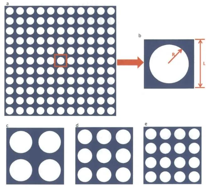
As was briefly mentioned in Section 2.3, we analyze infinite periodic structures for computational efficiency. Figure 3.1(a) shows an infinite periodic structure with circular holes. A unit cell is defined as the smallest repeating geometric unit of the periodic structure, as is

shown in Figure 3.1(b). A representative volume element (RVE) contains m x m repeating unit cells. Figure 3.1 (c)-(e) show RVEs of size 2 x 2, 3 x 3 and 4 x 4.

Since the infinite periodic structure is just the repeating of the unit cells, the void-volume fraction $ of the infinite structure can thus be defined as

1TR 2

(3.1)

where R is the radius of the circular void and L is the length of the unit cell square shown in Figure 3.1(b). To examine specimens with various void-volume fractions, we can simply change the ratio between R and L.

000000 000000*0 A L A

inuinuinumuinuinuinuinuuinuinl

r ~ r r ~ L A L Pr -I L d L A L Ad

I-Figure 3.1 (a) An infinite periodic structure with circular holes (b) Corresponding unit cell (c) Corresponding 2 x 2 RVE (d) Corresponding 3 x 3 RVE (e) Corresponding 4 x 4 RVE

b I

-t

e F, 19 F, '9 r- -I F, 'I F, -I F- -I F, 14 11 A

3.2 Analysis of instability

We analyzed three void-volume fractions

1

= 30%, 50% and 60%. Figure 3.2 shows the infinite periodic structures and the corresponding unit cells.

Following the procedure by Bertoldi and Boyce [1], Refined Eigen Analysis (Section 2.4)

was performed on RVEs consisting of m x m (m = 2,3, ... ,10) unit cells for all three

void-volume fractions, a total of 27 RVEs. All analyses were performed in ABAQUS/Standard using *BUCKLE module. The material model used was the Neo-Hookean model (Section 2.2) with a shear modulus of 0.058MPa. Infinite periodic boundary conditions (Section 2.3) with uniaxial loading were imposed. Triangular, quadratic plane strain elements (CPE6H) were used.

0 p p *000 00000000 00 000 00000 0 000000000 0 00000000000 01000000000 00000000000 00000000000 0 0000 00000 00000000000 00 000 0 * e U

se

U

ee

I U I

eeIIs

I I I

Figure 3.2 Infinite periodic structures and their corresponding fraction 4 = 30%, 50% and 60%

unit cells with void-volume

LU~ -L

T

L

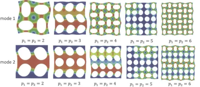
Figure 3.3 shows the first and second mode of * = 50% for cases where p = (2,2), p = (3,3), p = (4,4), p = (5,5) and p = (6,6).

4'

= 30% and 4' = 60% showed similar modes.

The figure clearly shows that eigenmodes of the RVE vary with the number of unit cells it consists of. Interestingly, the same first eigenmode exists for RVEs that consist of even

number of unit cells (i.e. p = (2n, 2n), n = 1,2 ... ). In other words, the first mode of a 6 x 6

RVE can be assembled by three 2 x 2 RVEs. This does not hold for either the second mode or the odd-sized RVEs. This observation suggests that the first mode of the even-sized RVEs is a result of local instability that occurs through the entire structure, causing the global periodic pattern transformation. Higher modes are not presented here as they are unlikely to occur due to their high critical loads. However, one may preferentially activate high modes by placing

inclusions in the voids. This is yet beyond the scope of this study and thus will not be discussed.

mode 1 16 P1 = P2 = 2 mode 2 P1 = P2 = 2 P1 =P2 =3 P1= P2= 3 P1 =P2= 4 P1 = P2= 4

Figure 3.3 First and second eigenmode for 4' = 50% for (5,5) and p = (6,6)

p = (2,2), p = (3,3), p = (4,4), p =

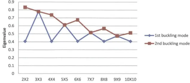
To quantitatively verify the above observation, we plot the eigenvalues against RVE size in Figure 3.4. As is clearly shown in the plot, even-sized RVEs have the same values for the

lowest critical load and hence are the preferred eigen modes. This indicates a repeating 2X2 first buckling mode throughout the structure.

P1 P2=

P1 =P2 5

P1= P2= 6

--- 1st buckling mode

-M-2nd buckling mode

2X2 3X3 4X4 5X5 6X6 7X7 8X8 9X9 1OX10

Figure 3.4 Eigenvalue vs. RVE size for ip = 50%. $p = 30% and q' = 60% showed similar trends with different eigenvalues.

3.3 Post-buckling analysis

From the Refined Eigen Analysis in the previous section, a 2 x 2 RVE was used for post-buckling analysis to obtain stress-strain data for post-post-buckling behavior. An imperfection in the form of the first buckling mode was introduced to preferentially activate the first mode. Figure

3.5 shows the stress-strain curve for each void-volume fraction.

35 1 - 'P =30% =50% ---

P

=60% 6 8 Nominal strain (%) 10 12 14

Figure 3.5 Nominal strain vs. nominal stress for $ = 30%, $ = 50% and

4'

= 60%

to MU 0.9 0.8 0.7 0.6 0.5 0.4 0.3 0.2 0.1 0 30 25 20 I 15 010 5 0 0 2 4

-'or-From the plot, we can see that:

(1) All three curves have three distinct regimes: a linear elastic response followed by a distinct rollover at a critical load followed by a much reduced slope (a near plateau like regime) This is clearly a result of the buckling at the critical load.

(2) Although all structures exhibited similar behaviors, a departure from linearity due to instability, their critical stress or critical strain at buckling were quite distinct.

3.4 Understanding the effect of void-volume fraction

The observations in Section 3.3 can be conceptually understood as follows.

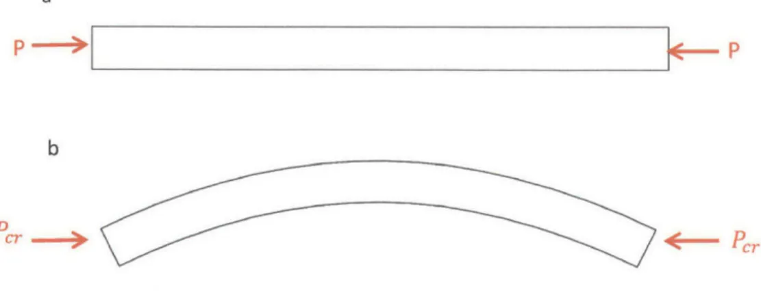
The ligaments between the voids can be viewed as small beam elements. Figure 3.6 shows a beam subject to compressive load and the first buckling mode of the beam when the load reaches a critical value.

From Euler beam buckling, the critical load for beam buckling with pinned-pinned ends is

nri Pr = EI(-) 2

L

where E is the Young's modulus, I is the moment of inertia and L is the beam length. a

(3.2)

I

iI

b

Pr --- v -- ~ Pcr

Figure 3.6 (a) A beam subject to compressive load (b) The first buckling mode of the beam when the load reaches a critical value.

Figure 3.7 shows the dimension of the beam with Young's modulus E. Let the symbol "~" denote "proportional to" or "scale as" and we conduct the following scaling

E t

d

Figure 3.7 Dimensions of the beam

The moment of inertia I is scaled as

(3.3) where d is the in-plane width of the beam and t is the depth.

Thus, the critical force is scaled as

I d3_t

Pcr~ -1 12W

where L is the in-plane length of the beam. Then, the cross-sectional area is scaled as

A-dt

(3.4)

(3.5) Hence, the critical stress

d3t

cPr

Pcr

~- d 2

A dt dt 1

(3.6)

The term d/1 is usually referred to as the slenderness ratio of the beam. As we can see, the critical buckling stress is proportional to the slenderness ratio of the beam squared, meaning the more slender the beam, the lower the critical stress it takes to buckle.

We apply this result to the understanding of the behavior of our periodic cellular structures. The internal ligaments between the voids can be modeled as beam elements. The effective beam length 1 can be approximated as the diameter of the void, while the effective beam width d can be approximated as the smallest distance between the voids. Hence, the

slenderness ratio of the ligament is also d/l. 1 and d are depicted in Figure 3.8 (a). Moreover, the relation between the critical stress of the local ligament and the macroscopic critical stress is depicted in Figure 3.8(b). The critical stress of the local ligament is the critical stress we described above in the beam analogy. It should be proportional to the slenderness ratio of the ligament. d

_-+31

d₁ d

4=30%--

0.67 1 1 d =50%,- = 0.25 d i~60%-T=O.14 acrmacro Ucrligament

Figure 3.8 (a) Inter-void ligament slenderness of RVE with different void volume fractions (b) relation between critical stress of the ligament and the macroscopic critical stress

When the whole structure is compressed, the ligaments experience mainly the

compressive load along their 1 direction. When the local compressive stress is below the critical value, the ligament behaves linearly as a normal linear elastic column, which explains the linear regime of the stress-strain curve. However, as the deformation becomes larger, the local

compressive stress reaches the critical value and thus all the ligaments buckle in a way similar to Euler beam buckling. This accounts for the critical stress followed by the stress plateau after the linearity.

To quantitatively look into the effect of the slenderness ratio of the ligament, we plot

acrjligament vs. in Figure 3.9. The values of ( and acr-ligament are normalized by their values at $ = 60%.

The void-volume fraction is related by the ratio of d/1 and the macroscopic critical stress is related to the local ligament critical stress; therefore if we plot the macroscopic critical stress vs. void-volume fraction, it follows the same trend as local ligament critical stress vs.

slenderness ratio. This is shown in Figure 3.10.

It can be clearly seen from Figure 3.8 that the inter-void ligament of

4,

= 60% is much longer and thinner than that of = 30%, or equivalently has a larger slenderness ratio, so it should buckle much earlier than $ = 30% and have a lower local and macroscopic critical stress. This conclusion is in good agreement with the stress-strain plot in Figure 3.5.

It is worth noting that critical stress is strongly affected by the void-volume fraction or the slenderness ratio, as is shown in Figure 3.9 and Figure 3.10. The macroscopic critical stress drops by nearly 70% when the void-volume fraction increases from 30% to 50%. This makes a huge difference in designing deformation-induced devices as will be explained in the following chapters.

U' 0 E U' 0U Z 4 3.5 3 2.5 2 1.5 1 0.5 0

ii

, 0

7l

1 2 3 Normalized d/l 4 5

Figure 3.9 normalized acrligament vs. d/li

(A 0 30 25 20 15 10 5 0 30% 50%

Void volume fraction

65%

Figure 3.10 Void-volume fraction vs. critical stress

3.5

Conclusions

Here, we summarize the important results from analyzing circular holes on a square lattice of varying void-volume fraction, as they are crucial to our design in the following chapters.

(1) An elastomeric periodic cellular structure comprising of square arrays of circular holes would suddenly transform into a periodic pattern of alternating and mutually orthogonal

ellipses (Figure 3.2) upon reaching a critical load. This dramatic shape change offers the opportunity for the design of tunable and deformation-controlled switches.

(2) The global dramatic pattern transformation is a result of the buckling of the inter-void ligaments.

(3) The void-volume fraction has a strong effect on the onset of buckling (i.e. critical stress and strain).

3.6 References

[1] K. Bertoldi, M. C. Boyce, S. Deschanel, S. M. Prange, and T. Mullin, "Mechanics of deformation-triggered pattern transformations and superelastic behavior in periodic elastomeric structures," J. Mech. Phys. Solids, vol. 56, no. 8, pp. 2642-2668, 2008.

Chapter 4

Micromechanical

model based

design of contact nubs

In this chapter, in order to make connections within the voids upon pattern transformation, we introduce a microstructural feature - contact nubs. It is reasonable to expect the response of the structure with nubs will be different from the one without the nubs due to the change in the microscopic structure. Therefore, to explore the effect of adding contact nubs on the structural behavior, finite element models were built and analyzed in the commercial finite element package ABAQUS. A series parametrical analysis was undertaken over different nub

geometrical parameters to test and optimize the nub geometry. The input file for ABAQUS was generated using MATLAB scripts.

In the following sections, the finite element model used, the nub design parameters and the simulation results are presented.

4.1 Conceptual design

In light of the conclusions drawn from Chapter 3, the periodic structure showed great potential for the design of instability-induced switches and yet one major challenge remains; how to utilize the dramatic shape change upon buckling. In this section, we present a novel design feature, which we refer to as the "contact nubs" to take advantage of the shape transformation of voids from circle to ellipse.

The difference between a circle and an ellipse is that an ellipse has one long major axis and one short minor axis while a circle has essentially an infinite number of pairs of "major" and "minor' axes of the same length. The design idea is simple, as shown in Figure 4.1. By adding a pair of nubs, we make the connection when the circular void on the left buckles into an elliptical void on the right, turning the sudden shape change into a real "switch".

Particularly, when the load is below the critical load, even though the circle is

compressed, the deformation is still relatively small so that the nubs are not in contact, which means the switch is off. Only if the load and the strain pass the critical value, the circular void would suddenly transform into the elliptical shape so that contact between the nubs is then

initiated, which means the switch is on. Since the material is elastic, this process can be repeated. Therefore, a switch that can be turned on and off via deformation is realized.

We also note that since the void shape is symmetric, we can add two pairs of nubs aligned vertically and horizontally, so that at least one pair of nubs can make contact regardless of the loading direction.

Figure 4.1 The conceptual design of contact nubs

4.2 Design parameters

The nub design concept is easy to grasp, however, adding nubs is essentially changing the microstructure of the periodic structure. It presumably could affect the instability response of the structure. Therefore, the effect of nub geometry on the buckling and post-buckling behavior of the structure needs further investigation.

Guided by engineering intuition, we identified three major geometrical parameters as shown in Figure 4.2.

A is the length of intersection between the nub and the inter-void ligament. B is the width of the nub end that makes the contact. C is the distance between the opposing nubs. Therefore, A is used to examine the effect of the connection between the nubs and the inter-void ligament. B is used to examine the contact between the mating nubs. C is used to examine the strain level at which the nubs make contact. A larger C means that greater strain or stress is required to achieve

contact. We also looked into the effect of all three parameters and their relationship with the void-volume fraction. The results are reported in the next few sections.

A

Figure 4.2 Nub design parameters

4.3 Effect of nub geometries for fixed void-volume fractions

From Chapter 3, we know that the critical load is strongly dependent on the void-volume fraction. Here, in order to examine solely the effec of nub geometry, we kept the void-volume fraction 4 = _{50% fixed and varied the parameters A, B and C. The focus here is still the}

eigenvalues and eigenmodes, or in other words, critical stress and strain. 4.3.1 Keep A constant while varying B and C

We still used 2x2 RVEs as we assume that there would be the same 2x2 periodicity as in the structures without the nubs. A total of nine structures were considered (see Figure 4.3). We normalized the parameters by R to make our studies applicable to different length scales.

The first buckling mode essentially follows that of the structure without the nubs; however, the eigenvalues are changed quite a bit due to the effect of the additional "nub"

material at the beam center which also aids in resisting buckling. Figure 4.4 shows the first mode of the specimen with A = 0.25R, B = O.5R, C = 0.6R. The nubs make connections after the structure buckles as expected.

B = 0.6R

C = 1.1R

C = R

C = 0.9R

Figure 4.3 Nub shapes with B = O.5R: O.1R: 0.7R, and C = 0.9R: O.1R: 1.1R while keeping A = 0.25R fixed

Figure 4.4 First mode of the specimen with Nub shapes with A = 0.25R, B = O.5R, C = 0.6R

B = 0.7 R B = 0.5R

Eigenvalues plotted against B with different values C are shown in Figure 4.5. As we can see, there is no significant difference between different values of B or C for a fixed A. However, the eigenvalue of the structure with nubs is about 10% higher than those of the structures without nubs. This can be interpreted as meaning that adding nubs is somehow equivalent to adding more material and stiffness to the inter-void ligaments, which gives rise to a higher buckling load.

Since B is the surface that makes the contact, we would want B to be as large as possible to ensure full contact between the nubs, as long as they do not touch each other during the process.

Since C determines when the nubs meet, we could easily tune the length of C to control the strain level at which the nubs make contact.

0.46 -4-C/R=1.1 __.44__-_C/R=1 0.44 C/R=0.9 0.42 Without Nubs 0.4 --0.38 -0.5 0.6 0.7 B/R

Figure 4.5 _{Eigenvalues vs. B for different values of C for a fixed A=0.25R}

4.3.2 Keep B constant while varying A and C

Having identified the effect of B and C, we now explore the design parameter A that relates the nub with the ligaments, through Refined Eigen Analysis of the 2x2 RVEs. A total of nine structures were considered in this section (see Figure 4.6).

A = 0.15R

C = 1.1R

C = R

E

C = 0.9R

Figure 4.6 Nub shapes with C=0.9R, R, fixed

A = 0.25R

E:3

A = 0.75R

1.lR, and A=O.15R, 0.25R, 0.75R, while keep B=0.7R

The results are shown in Figure 4.7. As predicted in Section 4.3.1, the parameter C plays no role in determining the critical stress. However, parameter A, on the other hand, has a strong effect on the buckling load. The eigenvalue increases by nearly 30% as A increases from 0.15R to 0.75R.

This gives us great flexibility for designing our structures. For example, we can control the width of A to obtain the desired critical stress, or vice versa. Also, the strain level at which the nubs make contact is solely determined by C. Therefore, by simply adjusting the distance C between the nubs, we could easily control the contact strain.

0.55 0.5 > 0.45 0.4 0.35 0.15 0.25 A/R

Figure 4.7 eigenvalues vs A for different values of C

4.4 Effect of void-volume fractions for fixed nub geometries

So far, we have examined the effect of nub geometry on material behavior at a given void-volume fraction. In this section, we evaluate the material response for a given nub geometry with the change of void-volume fraction. Three specimens with Ji = 20%, 50%, 70% were studied (see Figure 4.8). The nub geometry is the same for all three specimens with A =

0.25R, B = .5R, C = 0.9R.

ip=20% 0 = 50% 70%

Figure 4.8 The 2D unit cell with $f = 20%, 50%, 70%. Nub design parameters are A =

0.25R, B = 0.5R, C = 0.9R. 0.75 -$-C/R=1.1 -U'-C/R=1 C/R=0.9 Without Nubs

We compare the results with structures without nubs in Figure 4.9. The eigenvalues of all three structures are larger than their corresponding structures without the nubs. However, the

increase of eigenvalue is tremendously larger for structures with a small void-volume fraction.

-i C w 1 0.9 0.8 0.7 0.6 0.5 0.4 0.3 0.2 0.1 0 0.7% " with nubs * without nubs 236% 20% 50% Void-volume fraction 70%

Figure 4.9 Comparison of eigenvalues between structures with and without nubs

4.5 Design of contact nubs for circular holes on a hexagonal lattice

Previous sections explored the design of contact nubs utilizing the alternating, mutually orthogonal elliptical pattern of an elastomeric matrix with a square array of circular voids after buckling. It has also been found that different hole arrangements would result in different buckling patterns for porous elastomers [1], [2]. Figure 4.10 shows examples of two distinct buckling patterns resulting from different hole arrangements under uniaxial compression.

Figure 4.10 Two elastomeric porous structures with different hole arrangements buckle under uniaxial compression (Taken from Shim, Shan et al. 2013 [2])

The findings create more options for the design of our contact nubs, as the nubs do not necessarily need to be aligned vertically or horizontally. Their orientation can be tailored according to the buckling pattern.

Guided by the results in previous sections, we choose a nub design with A = 0.25R, B =

0.5R, C = 0.9R and the void-volume fraction is j = 50%. In this case, we simulated both a finite-sized specimen and its infinite periodic counterpart.

Figure 4.11 (a) shows a finite-sized sample with a 7X8 hexagonal array of circular holes with nubs while Figure 4.11 (b) shows a RVE representing its infinite periodic counterpart.

Note that the RVE was deliberately chosen as in Figure 4.11(b) for it to be compatible with our MATLAB code for periodic boundary conditions in x and y directions. There exist other choices of RVEs that may be more computationally efficient but require another set of scripts. Moreover, we want the RVE to have a complete void in the middle for better visualizing the deformation.

Also, the holes next to the edge of the finite-sized sample were cut in half to minimize the boundary effect.

Figure 4.11 (a) a finite-sized sample with a 7 x 8 hexagonal array a RVE representing its infinite periodic counterpart.

of circular holes with nubs; (b)

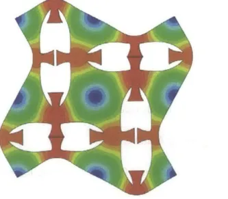
Figure 4.12 presents the first buckling mode of the structure. A different pattern from the matrix with holes on a square lattice is observed. The circular holes morphed into ellipse-like holes that alternate direction from row to row, clearly indicating a different mechanism from that of the square array. This distinctive pattern transformation is a result of critical intervoid shear instability, which is discussed in detail in Bertoldi, Boyce et al. 2008 [1]. An important

consequence of this shear instability mechanism is that the contact nubs which had been aligned were shifted due to the shear deformation and thus no connections were able to be made upon buckling. This is also expected to happen in matrix with a staggered array of voids.

- In a word, elastomeric matrix with a hexagonal or staggered array of holes is not suitable for the design of conductive pathways due the nub shifting resulting from shear instabilities.

Figure 4.12 (a) first mode of the finite-sized sample (b) first mode of the RVE

4.6 References

[1] K. Bertoldi, M. C. Boyce, S. Deschanel, S. M. Prange, and T. Mullin, "Mechanics of deformation-triggered pattern transformations and superelastic behavior in periodic elastomeric structures," J. Mech. Phys. Solids, vol. 56, no. 8, pp. 2642-2668, 2008. [2] J. Shim, S. Shan, A. Kosmrlj, S. H. Kang, E. R. Chen, J. C. Weaver, and K. Bertoldi,

"Harnessing instabilities for design of soft reconfigurable auxetic/chiral materials," Soft Matter, vol. 9, no. 34, p. 8198, Aug. 2013.

4M "Alio AOQ .4 jp%: ,Pp A PZ 444 ..... ..... -AV

Chapter

5

Micromechanical

model based

design of conductive pathways

In Chapter 4, we introduced a novel design feature which we referred to as "contact nubs" and demonstrated how connections are made when the circular holes transform into the elliptical shape. We also investigated the effect of nub geometry on the structural behavior. Thus far, however, we have not addressed the question on how to make connections between the voids.

In this chapter, we will introduce another design feature: the conductive pathways. By adding a conductive layer on the substrate, we are able to activate a conductive pathway when opposing nubs make contact. In general, the conductive path can be thermal, mechanical or electrical, but here, we will focus on the electrical conductivity for its application in flexible circuits.

5.1 Modeling rationale for thin film bonded to an elastomer substrate

To form electrical conductive pathways, or conductive patterns, the most common way is to bond a layer of thin film to the substrate. Traditionally, the film is made of metal for its high electrical conductivity. But recently, with advances in 3D printing technology and its application in printed electronics, conductive ink, a special ink that conducts electricity by adding silver nanoparticles or graphene into a solvent, is gaining more and more attention for its operational ease and printing flexibility.

When one material is adhered to another material (i.e. the thin film and the substrate in our case) upon deformation, several possible scenarios might happen due the mismatch in material properties of the two materials and the loading condition.

1) When the load is tensile and the film and the substrate are perfectly bonded with each other, they will either stretch together like a single material until one of them (usually the thin

film because it is stiffer and also has a smaller strain to break than the substrate) ruptures at a critical stress or strain, as shown in Figure 5.1(a).

2) When the load is compressive and the film and the substrate are still perfectly bonded with each other, wrinkling would happen (i.e. the film buckles into multiple sine waves) upon reaching a critical load, as is shown in Figure 5.1(b).

3) When the film and the substrate are not so well bonded, at some point of deformation, the film detaches from the substrate. This can happen i either compression or tension and is called delamination. Figure 5.1(c) shows that the film debonds and assists the rupture when stretched, while Figure 5.1(d) shows the detachment of the film during compression.

Film

b d

Figure 5.1 (a) A film stretches with the substrate when well bonded to the substrate. (b) A film wrinkles under compressive load when well bonded to the substrate. (Taken from Li, Suo et al. 2005[1]) (c) A film detaches from the substrate and ruptures under tensile load. (d) A film detaches from the substrate under compressive load. (Taken from Huang, et al. 2012)

Modeling a substrate with a film coating requires a full three-dimensional analysis. The film is taken to be perfectly bonded to the substrate and is modeled as linear elastic at all strain levels of our interest so that fracture will not occur. Given the above discussions, in the

following sections we will focus on the effect of elastic properties and geometrical features of the film on the 2D in-plane behavior of the structure. Note that the modeling space is in 3D because of the film layer.