Mantle heterogeneities, geoid, and plate motion: a Monte Carlo inversion

HAL Id: hal-02046607

https://hal.archives-ouvertes.fr/hal-02046607

Submitted on 22 Mar 2021

HAL is a multi-disciplinary open access

archive for the deposit and dissemination of

sci-entific research documents, whether they are

pub-lished or not. The documents may come from

teaching and research institutions in France or

abroad, or from public or private research centers.

L’archive ouverte pluridisciplinaire HAL, est

destinée au dépôt et à la diffusion de documents

scientifiques de niveau recherche, publiés ou non,

émanant des établissements d’enseignement et de

recherche français ou étrangers, des laboratoires

publics ou privés.

Mantle heterogeneities, geoid, and plate motion: a

Monte Carlo inversion

Y. Ricard, C. Vigny, C. Froidevaux

To cite this version:

Y. Ricard, C. Vigny, C. Froidevaux. Mantle heterogeneities, geoid, and plate motion: a Monte Carlo

inversion. Journal of Geophysical Research, American Geophysical Union, 1989, 94 (B10),

pp.13,739-13,754. �hal-02046607�

MANTLE HETEROGENEITIES, GEOID, AND PLATE MOTION:

A MONTE CARLO INVERSION

Yanick Ricard, Christophe Vigny, and Claude Froidevaux

D•partement de G•ologie, Ecole Normale Sup•rieure, Paris

Abstract. Seismic tomography in both the up-

per and the lower mantle, as well as subducting oceanic slabs defined by seismicity, has been translated into density heterogeneities to gener-

ate models of mantle circulation. These models

can predict both the surface velocities and the geoid, which can be compared with plate tectonics

and gravity data. A given model is specified by 6

parameters related to the viscosities of 3 mantle layers and the absolute amplitudes of density variations in the upper and lower mantle as well as in the slabs. The values of these parameters are chosen at random within an acceptable range. Each model is submitted to an appropriate test comparing observations with predictions. The re- sults of the most successful models selected by this Monte Carlo inversion are displayed. They

yield preferred mantle viscosity structures exhi- biting large variations at depth. With a physical

interface between upper and lower mantle, i.e.,

with the possibility for the circulation to pen- etrate the 650 km discontinuity, two classes of

viscosity profiles stand out. The first one im- plies a regular increase of the viscosity in the sublithospheric mantle, with reasonable values for the density parameters. The second one is un- expected in the sense that it predicts a very stiff bottom for the upper mantle. It also re- quires vanishingly small amplitudes for the upper mantle density heterogeneities defined by tomo- graphy, which would thus have to be of lithologi- cal rather than thermal origin. With a chemical

interface at 650 km the outcome is very similar:

the same two classes of viscosity structures do

yield a satisfactory geoid prediction. However

only the class of models with a stiff layer at midmantle depths predicts acceptable surface vel- ocities. Altogether the best models out of some

60,000 which have been tested only explain one third of the geoid and two thirds of the surface divergence for spherical harmonic degrees 1 to 6. Nevertheless the main features of these two ob-

served patterns are present in the computed maps,

and 4 out of 6 correlation coefficients lie close to the 90% confidence level. This is true for the geoid as well as for the surface divergence of the displacement velocity. However, as the inter-

nal viscosity structure has been assumed to have

spherical symmetry, the rotational component of

the surface velocities cannot be predicted.

Introduction

The geoid is an equipotential surface of the

Earth's gravitational field which practically co- incides with the mean surface of the oceans. Its

Copyright 1989 by the American Geophysical Union. Paper number 89JB00960

0148-0227/89/89JB-00960505.00

deviation from an ellipsoidal shape reveals the

existence of lateral density variations at all

depths and scales. The most prominent undulations

are at long wavelengths. At first sight, they ex- hibit no clear correlation with surface features:

hence their great interest for theoretical geo-

dynamics. The seismic tomography picture of the Earth's mantle which has emerged in recent years

provides a new data set which can be used to understand mantle dynamics and its surface ex- pressions, in particular gravity and plate veloc-

ities. A first level of physical understanding of these observables has now been established.

The distribution of seismic velocities reveals

lateral variations of a few percent in the upper

mantle [Woodhouse and Dzfewonskf, 1984; Nata• et aZ., 1986; Tanfmoto 1986] and about 1% in the lower mantle [Dzfewonskf, 1984]. The spatial res-

olution corresponds to spherical harmonic degree

6 or 8, i.e., at best to some 5000 km of lateral extent. Radially, the resolution varies from 100

km at shallow depths to more than 500 km near the core boundary. By assuming that these observed

patterns reflect temperature fluctuations, one

can identify low (high) density anomalies with regions of slow (fast) wave propagation. A first

attempt to predict the shape of the geoid on the basis of these deep density structures alone led

to a promising but puzzling result: the corre-

lation between observed and computed geoid for the lower mantle sources was significant for de-

grees 2 and 3, but negative [Dzfe•onskf, 1984]. No correlation was found for higher degrees or

for upper mantle sources.

The negative sign of the predicted long wave- length geoid can be removed by considering dy-

namic mantle models with internal loading [Rfcard

et

aZ., 1984; Richards and Hager, 1984; Lago and

Rabinowicz, 1984]. The internal loads induce a

circulation which deflects the existing density interfaces such as the core-mantle boundary and the outer surface. The amplitudes of these topo- graphies are very sensitive to the assumed radial

viscosity structure. They generate additional

contributions to the gravity field, not all with

the same sign. For a viscosity contrast between upper and lower mantle not larger than 30 the dy- namically induced deflection at the Earth's sur-

face yields the dominant term. Its sign is oppo- site to that of the deep source: hence the nega- tive correlation between this deep density struc-

ture and the geoid. On the contrary, a stiffer lower mantle can sustain internal loads with more efficiency so that the induced surface deflection

is much weaker. In this case, internal sources could indeed directly determine the sign of the geoid.

The relevance of dynamic Earth models predic- ting observables such as the geoid and the sur-

face velocities strongly depends upon two in-

gredients. Firstly, the capability of the physi-

13,740 Ricard et al.: Mantle Heterogeneities, Geoid and Plate Motion

cal model to reflect mantle processes realistic- ally. This will be discussed later. Secondly, the quality of the data defining the internal loadsß This raises the question of the validity of the tomographic data, and of the choice to make when

several sets are availableß For the lower mantle,

we had no choice as only one model is published,

even though another one [CZayton and Comer, 1983]

has already been used for the same purpose [Hayer et aS., 1985]. For the upper mantle the three models available include one [Tanimoto, 1986] which is preferred by some authors [Rfchards and Hayer, 1986] but not by us because it ignores crustal corrections and shows little correlation at shallow depths with structures like oceanic ridges or cratons. The other two models [Nataf et aS., 1986; Woodhouse and Dziewonski, 1984] detect these expected warm or cold tectonic provincesß They contain other common features, for example, under the Red Sea or Central Pacific areasß Late- ly the model by Woodhouse and Dziewonski has been confirmed by the analysis of an even larger set of seismic data [Dziewonski and Woodhouse, 1988]. This determined our selection.

The uncertainty of the tomographic models be- comes larger at higher harmonic degrees. On the other hand the lower degrees are enhanced when the geoid is computed. The most prominent fea- tures of the geoid are thus not very sensitive to uncertainties of the tomography at high degrees. Additionally one should remember that the power spectrum of the observed geoid starts at g = 2 and strongly falls as g increases.

The prediction of the geoid components of de- grees Z = 2 and 3 on the basis of lower mantle tomography alone is best for an Earth model where the mantle viscosity increase at 650 km is not

larger

than 10 [Hayer and Rfchards, 1984; Rfcard

et aZ., 1985; Hayer et aZ., 1985]. Such a small viscosity contrast between upper and lower mantle agrees with the conclusions of post-glacial re- bound [Wu and Peltier, 1982] and Chandler wobble studies [Yuen et aZ., 1982]. The predicted ampli- tude of the geoid is also satisfactory when the assumed proportionality between seismic velocity v _p and density p falls within the range of ex-

perimental

values

(0v./0p

= 3-4

km

s

-1 / g cm-3•

The above results i•ply a 650 km discontinui

mantle is purely physical. In models where this interface marks an intrinsic density step, the

flows above and below are separated but coupled.

One then speaks of a chemical boundary. Such models are not quite as successful in matching the geoid amplitude with the low degree mass het- erogeneities of the lower mantle [Hayer et aZ., •985].

For the upper mantle the tomographic model is

given in terms of A v 2 [Woodhouse

and Dzfemonskf

1984] We simply assume

that A v 2 = 2 vs A v s

where v s is taken from the Preliminary reference earth model (PREM) [Dzfemonskf and Jnderson, 1981] and varies with depth. The importance of density heterogeneities in the upper mantle thus

depends upon the value of 0vs/•.

The poor corre-

lation with the geoid suggests that the velocity distribution above 650 km could be linked to both temperature and chemistry fluctuations. However one specific correlation is noticeable: the long

wavelength geoid is always high over subduction zonesß Unfortunately, global tomography is not yet capable of detecting the subducting slabsß

Their excess mass characterized by a parameter

LAp, where L is the lithospheric thickness, can

be inserted in dynamic Earth models to compute a

geoidß The result is particularly well correlated with observations for degrees I = 4 to I = 9, if one assumes a very large viscosity contrast at 650 km, say more than 100 [Hayev, 1984]. As this stiff lower mantle is capable of supporting the weight of the dipping slabs, the induced surface depression is negligible and the gravity signal has the si•n of the excess density of the slabß This result however contradicts the conclusion of a rather uniform mantle viscosity deduced from

lower mantle loadingß

The tomography data set has recently been used

in conjunction with dynamic Earth models in order

to predict not just the geoid but also the sur- face velocities [Forte and PeZtier, 1987]. The latter can be compared with known plate veloc- ities. This new approach has the advantage of being sensitive to the absolute value of mantle viscosity. It yields a satisfactory pattern for the divergence of the surface velocity field near oceanic ridges. The convergence zones however cannot be correctly predicted, most likely be- cause of the lack of tomography signal associated with the subducting oceanic slabs. The required viscosities (2x1021Pa s in the upper mantle) are close to those derived from post-glacial rebound and the increase within the lower mantle is not

more than one order of magnitude. An additional

test could easily be performed by including the contribution of the slabs to the total internal loads. These slabs are indeed known to be of prime importance for plate dynamics [Forsyth and Uyeda, 1975; Rfchardson et aS., 1979].

All Earth models described above, as well as

those which will be found in the present paper, have one major limitation: they assume a purely radial viscosity structure, i.e., they forbid the very existence of lithospheric plates with their weak boundaries. The predicted surface velocity field is therefore purely poloidal, i.e., without any shear or toroidal component. For the real Earth both components are equally excited [Hayer and O'ConneZZ, 1979]. Some first models including lateral viscosity variations inside the outermost shell of the Earth are now available [Rfcard et aZ., 1988]. They predict several features of the geoid such as the marked maxima over convergence zones, and weaker minima over the softer ridge structures. In the present paper, however, no attempt will be made to include similar depar- tures from spherical symmetry in the viscosity distribution.

We shall perform a series of tests using our

selection of available data for internal loads

(tomography and slabs) and the present state-of- the-art dynamic Earth models with a purely radial viscosity distribution. In order to investigate as large a variety of viscosity values as poss- ible, we have established a straightforward Monte Carlo inversion procedure. The predictions of each model are compared with the real geoid and plate velocity divergence for degrees between 1 and 6. The best fitting models out of some 60,000 are then selected and discussed. The Monte Carlo

approach was already introduced in geophysics in order to construct elastic Earth models satisfy- ing seismic observations [Press, 1970].

Monte Carlo Selection

We use the tomography data set L02.56 for the lower mantle [Dzfewonskf, 1984]. It includes de- grees Z = 1 to 6. For the upper mantle we take the M84C set of data [Woodhouse a•d Dzfewonskf, 1984] truncated beyond Z = 6. To this we add a file describing the density anomalies associated with the seismic portions of subducting slabs. This file was provided by B. Hager who made use of it for some of his own models [Hager, 1984].

To convert the above spatial distributions

into densities we need the values of three para-

meters: LAp, •vs/•p, and •vp/•p. The second

de-

rivative

was proposed to amount to 3-4 km s -1 /

gcm -3 by comparing the observed low degree geoid

and that predicted by a model with internal load- ing restricted to the lower mantle [Hager et aZ., 1985]. Experiments with the relevant oxides and

silicates yield values of •Vp/•p between

3 and 10

km s -1 / g cm

-3

[Sumfno and Anderson, 1984]. In

our models, we allowed this derivative to vary

from 1 to 13 km s -• / g cm

-3 . The same laboratory

measurements indicate a value around 3 km s -• /

gcm

-3 for Ovs/O

p. In order to allow for a poss-

ible chemical rather than thermal origin of the velocity variations in the upper mantle, we let

this parameter vary from 1 to 80 km s -1 / gcm -3.

The large value of the upper bound tends to damp the density fluctuations, i.e., to attribute the

observed seismic pattern to a possible petro-

logical distribution without associated density

changes.

The free parameter LAp for the slabs can be estimated by comparing the bathymetry of ridges

to that of old ocean floors. Isostasy requires

L ZSp to be equal to the increase in water depth, say 4 km, times the density difference between

mantle rocks and water, say 2300 kg m

-3 . In our

dynamic Earth models we therefore allowed the

value

of LAp to vary between 3.0x106 and

1.Sx107 kg m -2 . The lower bound corresponds to a situation where the added slabs have a small den-

sity contrast and are not essential in the model. This could also be interpreted as an indication that their signature is already present in the

tomography signal. The upper bound, on the con-

trary, would suggest that the dense slab struc-

ture could extend beyond the seismicity limit, as suggested by wave propagation analysis [Creager and Jordan, 1984]. Another possible parametriz- ation would thus consist in varying the length of slabs rather than their density [Hager, 1984].

This alternative is not equivalent to the choice made in this paper, in the sense that the Green

function relating the loads to the induced geoid can change markedly with depth. The density dif- ferences represented by the subducting slabs are certainly of large magnitude, but very localized. Therefore their amplitude content at degrees 2 to 6 of spherical harmonics is indeed rather weak in comparison with the density heterogeneities de-

fined by upper mantle tomography. For 8vs/8 p = 5

km s -• / g cm

-3 and a slab thickness L = 100 km,

seismic tomography yields density fluctuations of

amplitude 0.05 g cm -3 at 300 km depth, whereas the additional contribution derived from the ex-

isting slab configuration amounts to 0.08 g cm

-3 .

For a given internal density•d!stribution,

the

geoid N and surface divergence V.v of the induced flow can be computed for any chosen viscosity

profile within the sublithospheric mantle. Here

we assume a reference viscosity 40 in the upper 100 km, and divide the remaining mantle in three layers with interfaces at depths of 300, 650 and

2900 km, and with viscosities 4•, 42, and 43,

respectively. These viscosities are allowed to

scan several decades: 4• can vary between 40 and

10-• 40, 42 has a broader range from 103 40 to

10-4 40 , while in the lower

mantle

43 Can

take

values between 10 40 and 10 -3 40. Both physical

and chemical interfaces at 650 km have been con- sidered, depending upon the possibility for the induced flow to cross this boundary. The general formalism is fully described in recent papers

[Rfcard

et aZ.,

1984; Richards and Hagen, 1984;

Forte and PeZtfer, 1987] and consists in comput- ing Green excitation functions for each spherical harmonic degree. A convolution of the Green func- tion with the radial load distribution is then carried out for every degree Z and order m. This yields the computed coefficients øNzm for the

geoid and c(V.v)zm for the surface velocity

divergence.

Each dynamical model we computed includes six

free parameters:

LAp, •vs/•p, •v•/•p, 4•/40,

42/40, and 43/4 o . As our expansion

•n spherical

harmonics is limited to degree 6, a given model predicts 45 geoid coefficients (degrees 2 to 6) and 48 velocity divergence coefficients (degrees

Z = I to 6). Notice that the viscosity 40 of the

outermost layer has a prescribed reference value. The value of the geoid reflects the force equi-

librium between applied loads and induced inter-

face deflections. It is sensitive to the viscos- ity structure, but not to the absolute value of

the viscosi•y• On the contrary, the absolute am-

source load intensity and absolute value of the

viscosity. If one restricts the comparison be-

tween modeled and observed velocities to the in- dividual correlation coefficients one can only determine viscosity ratios for the structure as well as density ratios for the loads. Our pro- cedure is restricted to relative velocity values in order to avoid the difficulties associated with the unsolved problem of the equipartition of energy between poloidal and toroidal fields.

For a given model the above six free para-

meters are chosen within each of the allocated

ranges of values. Two selection criteria are then calculated in order to determine the best poss-

ible models. It is usual to consider the correla-

tion coefficients between computed models and

observations for each degree. However, a good correlation at all degrees does not imply a sat- isfactory prediction of the amplitudes or of the global shape. On the other hand, the confidence level of a global correlation including all de- grees together is only meaningful when the coef-

ficients of the spherical harmonics do not de-

crease too sharply in amplitude as Z increases. This last condition holds for the velocity di- vergence V.v, but does not apply to the geoid N

13,742 Ricard et al.: Mantle Heterogeneities, Geoid and Plate Motion

[KauZa, 1966]. One thus defines two different selection criteria: _<6

c v =

(•)

c• = 4•

N•m+øN•m

<1

1/2

o

Here the upper index o refers to observations, as c stands for computed values. The first cri-

terium C

v corresponds to the correlation coef-

ficient for V.v. It includes all degrees from

Z = 1 to 6. A good model yields a maximum value

of Cv,Close to unity. The second criterium C

N ex-

observed and predicted geoid. This residual vari- ance is given in meters, and can thus be compared with the average amplitude of the total geoid when degrees Z = 2 to Z = 6 are taken into consi- deration, which amounts to 41 m. A good model should minimize the misfit given by the value of

C

N. By inspection of the above formula one sees

that a minimum

C

s requires maximum

values for all

correlation coefficients calculated for each de- gree as well as globally for all degrees. Quanti-

tatively

the value of CN is obviously dominated

by the largest coefficients, i.e., those of de- grees 2 and 3 which have average amplitudes of 33.7 and 19.2 m. For degrees 4, 5 and 6, this am- plitude drops to 10.0, 7.6 and 5.5 m.

Models With Internal Loading

In this section we mainly examine the results

of the selection procedure based on the best fit

to the geoid, according to criterium C

N. In order

to reduce computing time we usually ran some 3000

models with random values of the six free para-

meters described above. The allowed values in this random selection are regularly distributed on a logarithmic scale for the viscosities and on

a linear scale for the densities. For each para-

meter the allowed range was then cautiously re- duced around the group of values corresponding to the best 100 solutions. A new set of 3000 models

was then tested. This procedure was repeated six

times and satisfactory convergence was achieved. The first steps of the Monte Carlo selection re- vealed the existence of two classes of solutions for the mantle viscosity structure. For class 1 the viscosity stratification implies changes by

less than two orders of magnitude. For class 2 a strikingly stiff layer is found at the bottom of the upper mantle, with a viscosity contrast of

order 104 . For clarity these two types of sol-

Class 1 Solutions: Geoid

Figures 1 and 2 each depict the 15 best sets of free parameters selected for a mantle having

either

a physical or a chemical interface at 650

km depth. For class 1 the viscosity between 300 and 650 km is not allowed to take values much in

excess of that of the 100 km thick lithosphere. In both cases the fit is somewhat satisfactory,

as C• amounts

to 31 m. Thus 24%

of the real geoid

up to degree 6 is explained by the best models. By comparison the best two-layer model of Forte

and PeZtier [1987]

yields a mean discrepancy C•

of 33 m for degrees up to 5 only, and a weaker viscosity contrast. Here the selected viscosity structure of Figure 1 singles out the presence of a stiff lithosphere with a reference viscosity •0 and exhibits a marked jump by a factor of 50 be- tween upper and lower mantle. In Figure 2, i.e.,

in the presence of a chemical boundary at 650 km,

the structure is more homogeneous, except for a narrow asthenospheric channel. The upper histo- grams in both figures show that the density of the slabs is not well resolved by the models. In Figure 1, the partial derivatives of the seismic velocities are on the contrary well defined, as seen in the middle and lower histograms. The pre-

ferred values of •Vs/•p are well within the range

of experimental results and thus seem to rule out a predominantly petrological explanation for the

observed distribution of seismic velocities in

the upper mantle. For the lower mantle our pre-

ferred value of •Vp/•p is higher by 50%

than that

found by previous authors [Hager et al., 1985]

and remains compatible with experimental values

[Sumfno and Anderson, 1984].

In Figure 2, the

middle histogram still favors a thermal rather than a petrological origin for the upper mantle

heterogeneities. The low value of •vp/•p in the

lower histogram points to the presence of density heterogeneities of large amplitude in the lower mantle.

It is customary to plot the correlation coef- ficients between predicted and observed spherical harmonic coefficients degree by degree. This is done in Figure 3 for the geoid. The squares cor- respond to the best solution among the 15 given

in

Figure 1 for

a physical

interface.

For this

solution the 6 parameters take the values 0.003, 0.0035, and 0.25 for the three viscosity ratios,

and 9.6x106 kg m-2, 5.0 km s-1 / g cm-3, and 6.0

km s- 1 / g cm- 3 for the density coefficients.

No-

tice that for Z = 2, 3, 4, and 5 the coefficients lie close to or above the line of 90% confidence level. This statement alone could be misleading, because as mentioned above this best solution ex-

plains only 24% of the geoid mean amplitude. This

illustrates the general remarks we made before

defining C

v and C•: a good correlation between

orders is certainly required, but the amplitudes for all degrees must also coincide. This last aim is not quite reached yet. In the same figure the circles correspond to the best solution included

in Figure 2 for a chemical interface. Here the 6

VISCOSITY 1 E-04 SLABS

1'2 15

io

4'o 2'o

o

z

13 1•

7

4

1

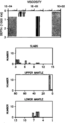
Fig. 1. Set of six free parameter values corre-

sponding to the 15 best solutions selected by a Monte Carlo method. The model Earth has a 100 km

thick lithosphere with viscosity

•0 = 1,

and 3

650 km interface between upper and lower mantle: this sort of interface is called physical. Each solution yields a computed geoid which has been compared with the observed one by means of (2).

The upper diagram depicts the selected viscosity

profiles within a prescribed range limited by the

shaded domains proper to class 1 solutions. Below this, 3 histograms describe the distribution of

1.6, and 2.0 with the same units as above. Notice that although these correlation coefficients are different from the previous ones, this solution also explains a sizable portion (24%) of the ob-

1 E-03 VISCOSITY 1E+oo 1E+03 ...,..J ..., .... ! ...,..J ...,..J ...,..J ...,... II III II '

II

o

pi.,

80

6'0 40

20

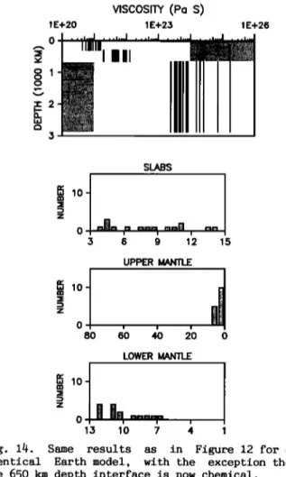
0

Fig. 2. Same as Figure 1, but for model Earth structures with a chemical interface at 650 km,

i.e., in which the circulation is not allowed to

cross that boundary . Notice that the low viscos- ity is only present in the upper part of the up- per mantle. The lower histogram points to a strong contribution from lower mantle heterogen-

the best values for density parameters. The upper

eities.

one gives the number of solutions versus the

value of the slab parameter LAp expressed in 106

kg m -2 . This parameter is not well constrained. Similarly the middle histogram is for upper mantle heterogeneities: the horizontal axis give

the allowed values of Ov

s/Op inkm s- 1 / g cm - 3 .

Notice that 14 solutions out of 15 happen to have the same value for this parameter. Finally the

lower histogram is drawn relative to Ovp/Op

for

the lower mantle. The best solutions are grouped

around 6 km s-i/

g cm

-3 . The orientation

of the

abscissae for each histogram is such that a se-

lected parameter value located on the left hand side corresponds to a smaller amplitude of the density anomaly than one located on the right

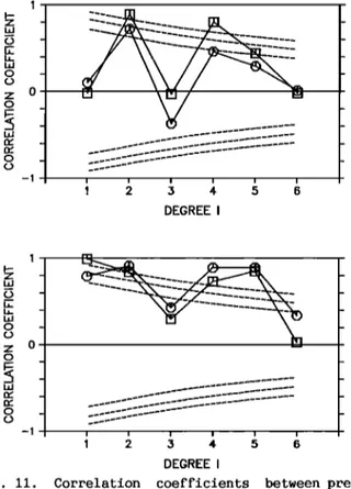
1 b_ L•_ W z w -1 DEGREE I

hand side. For oceanic slabs the most probable Fig. 3. Correlation coefficients for spherical

value of LAp lies in the middle portion of

the

harmonic degrees 2 to 6 between computed and ob-

horizontal axis. Experimental values of the de- served geoid for the best solution without rivatives of seismic velocities versus density (squares) or with (circles) a chemical interface also lie in the middle portion of the horizontal at 650 km. The three pairs of dashed curves indi-

axis of the lower histogram, but are at the ex-

cate

confidence levels

of 80,

90 and 95%, re-

13,744 Ricard et al.: Mantle Heterogeneities, Geoid and Plate Motion

..:...:::

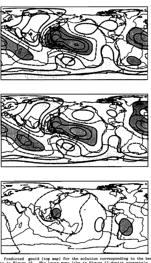
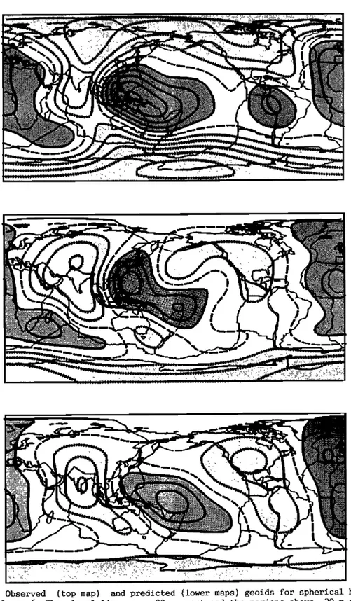
Fig. 4. Observed (top map) and predicted (lower maps) geoids for spherical harmonic

degrees 2 to 6. The level lines are 20 m apart and the regions above 20 m or below

-20 m are heavily or lightly shaded. The middle map derives from our best class 1 sol-

ution with a physical interface

at 650 km. It thus corresponds to one of the set of

six parameters included in Figure 1 and to the correlation

coefficients of.Figure 3

(squares). The lower map corresponds to the best solution with a chemical interface at

650 km, and is similarly related to Figures 2 and 3 (circles).

served geoid. If one computes the three separate

and upper mantle sources are equally important,

contributions

from slabs, upper mantle and lower

but the slab contribution is still

negligeable.

mantle one finds that the last one is largely

The hydrostatic geoid truncated above degree 6

dominant. This is not true for the model includ-

is

plotted at

the top of Figure 4 and compared

and lower maps depict the computed geoids for a

mantle with physical or chemical interface at 650 km. They thus correspond to the two sets of cor- relation coefficients of Figure 3. Visually, the

main equatorial maxima over Africa and western

Pacific are well predicted, as is the trough of

minimum amplitude over India. The main shortcom- ings are in the insufficient polar flattening and

in the absence of a maximum over South America.

CZass 2 SoZutions: Geoid

These solutions were isolated from those de-

picted in the above section by imposing a lower bound to the possible values of the viscosity be-

tween 300 and 650 km. This lower bound is ident-

ical with the upper bound imposed to the class 1

solutions. Figure 5 depicts the new best 15 sets of selected parameters for a physical interface at 650 km. The most striking feature is a very

stiff bottom layer for the upper mantle. It damps

the flow velocities at this level. There is thus not much difference in dynamical behavior with a model mantle having a chemical interface and the same stiff layer. These last solutions were also found, and are indeed quite similar, as seen in Figure 6. The other remarkable feature depicted

by the histograms of Figures 5 and 6 is the good

definition and high value for slab densities, the

VISCOSITY

1E-03 1E+00 1E+03

0 ...

LL[I,!!!l

...

•

9

12

15

Fig. 5. Same as Figure 1, but for the 15 best class 2 solutions. For this class the shaded area

shows that the bottom oC the upper mantle is al-

lowed to exhibit high viscosity values. Here the

selected density parameters in the histograms show that the preferred solutions imply very dense subducting slabs.

1 E-03

VISCOSITY

1E+oo 1E+03

, ,., .... I , ,,i..J . . . ,..J i i.,..J . ..I..J . ..,...

SLABS UPPER MANTLE

;o

2'o

o

z o I

Fig. 6. Same as Figure 2 but for the 15 best

class 2 solutions. As in the case of a physical

interface (Figure 5) the slabs are dense with a very well defined distribution.

vanishing amplitudes of the other density hetero- geneities in the upper mantle and the rather weak heterogeneities in the lower mantle. The best two solutions among those shown in the last figures correspond to a residual geoid of 28 m in both cases. Therefore it explains 32% of the observed geoid. The six free parameters amount to 0.018 (respectively 0.039), 260 (875) and 0.83 (0.82)

for

the viscosities,

and 15x106 (respectively

15x106) kg m

-2, 67 (70) km s -• / g cm -3, and 8.2

(9.7) km s -• / g cm

-3 for the densities.

The cor-

ted quantities are given on Figure 7. By compari- son with Figure 3 one notices that the class 2 solutions give a better fit than those of class 1, as can also be appreciated from the already

mentionned values of CN (misfit of 28 instead of

31 meters). Figure 8 maps the predicted geoid for

these best class 2 solutions. They are very simi-

lar. By comparison with the class 1 solutions of Figure 4 one notices a slight improvement over South America and the persisting weakness of the

polar flattening.

Predicted Surj•ace Velocities

We now turn to the problem of constructing dy-

namical Earth models with the same internal loads as above, but with the purpose of predicting the observed velocity divergence of plate tectonics.

13,746 Ricard et al.' Mantle Heterogeneities, Geoid and Plate Motion 1 b_ - W 0 - Z 0 w n• _ 0 - DEGREE I

Fig. 7. Same correlation coefficients as in Figure 3, but for both best class 2 solutions. Squares are again for a model Earth with a physi- cal interface at 650 km, and circles for a chemi- cal interface.

basis

of maximizing the correlation

criterium C

v

variations, we have fixed a scaling factor for

the loads by taking L •

= 107 kg m

-2. As already

noticed by Fo•te and Pe•tf• [1987] the predicted

surface velocities are not very sensitive to the relative radial variations of the viscosity. Both best solutions for a physical or chemical inter-

face at 650 km tend however to exhibit a stiff

layer at the botom of the upper mantle, as was the case in class 2 solutions for the geoid. Moreover these solutions lead to high values of the two derivatives related to upper and lower

mantle densities. This means that the role of the

slabs is enhanced with respect to that of density heterogeneities derived from seismic tomography.

Our best solutions yield a value of 0.82 for C

v .

Taking account of the 48 harmonic coefficients

involved here, this means that with an adequate

value of the reference viscosity •0, 82% of the

than 99,9%.

As the inversion for the velocity turns out to have less resolving power for the mantle viscos- ity distribution than that obtained by fitting the geoid, we now turn to a different approach. It consists in computing the surface velocity di- vergence for the solutions used to predict the best geoids of class 1 and 2. In Figure 9 the top

map depicts the observed velocity divergence for

Fig. 8. Maps of the predicted geoid corresponding to the best class 2 solutions. The top map is for an Earth model with physical interface at 650 km; the lower one for a

chemical interface at the same depth. These maps can be compared to those of Figure 4,

in particular to the top one corresponding to the observed geoid. The spacing between

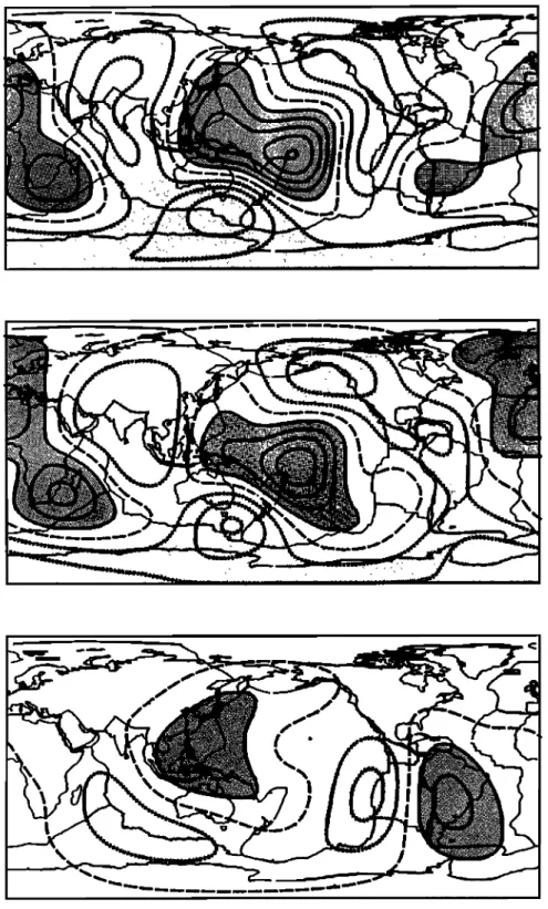
Fig. 9. Divergence of surface displacement velocities for spherical harmonic degrees

1 to 6. The top map corresponds to observed plate

velocities

with marked maxima over

oceanic ridges (heavy shading) and minima over subduction zones (light shading). The other two maps depict predicted values for our best class 1 solutions. Each map is normalized and has 5 level lines. The middle one gives the velocity divergence pre- dicted on the basis of the solution used to plot the middle geoid in Figure 4. It ac-

counts for 44% of the observed velocity

pattern. The lower one only accounts for 26%

13,748 Ricard et al.: Mantle Heterogeneities, Geoid and Plate Motion

Fig. 10. Same as Figure 9 but for our two best class 2 solutions, i.e.,

either with

(top) or without (bottom) chemical interface at 650 km. They respectively account for

56% and 64% of the observed pattern depicted at the top of Figure 9. In the lower map,

the spurious zone of opening along about 90 ø longitude has a size which is exaggerated

by the cylindrical

projection. The convergence

along the rim of the Pacific is well

predicted as are the major oceanic zones of opening.

degrees I = 1 to 6. The middle and lower maps are predicted on the basis of the best solutions of class 1, first with a physical and second with a chemical interface. They correspond to geoids de-

picted

in Figure 4. Our middle map is very simi-

lar to the preferred model of Forte and Peltfer [1987] based on a two-layer mantle, and accounts for 44% of the observed pattern. This resemblance

can be explained by two reasons' (1)4 •he weak

sensitivity of the Green functions of V.v to the radial viscosity variation, and (2) the absence

or relative weakness of the internal loads corre-

sponding to oceanic slabs in both investigations. The lower map only accounts for 26% of the obser- vations. Notice that the computed maps have the

correct localization for the zones of opening

corresponding to oceanic ridges. However they lo- cate the zones of convergence beneath old dense cratons like Africa, South America, Australia, North America and Siberia.

Figure 10 corresponds to the best class 2 sol- utions already used to draw the predicted geoids in Figure 8. These velocity divergence maps pre-

dict 56%, respectively

64%, of the real pattern,

a remarkable improvement. A comparison with Fig- ure 9, which depicted the class 1 solutions, il-

lustrates this point: convergence in the Western Pacific region has advantageously replaced the spurious downwelling of old cratons. This is of course not a surprise as the main driving force has been shifted to the slabs (see upper histo-

grams in Figures 5 and 6). Figure 11 depicts the

vergence corresponding to the above class 1 and class 2 solutions.

Models With Both Internal Loading

And Imposed Surface Kinematics

The previous section showed that it is quite difficult to propose dynamic Earth models which satisfactorily predict both the geoid and the di- vergence of plate velocities. In particular, the relative importance of slabs and other mantle heterogeneities is not always the same for both criteria. Generally speaking the prediction of the velocity divergence has been more successful than that of the geoid. Now we shall consider the possibility of taking observed surface velocities

in addition to internal loads as given contraints

to compute the induced mantle dynamics and the associated geoid. Plate tectonics velocities con-