HAL Id: hal-03256356
https://hal.archives-ouvertes.fr/hal-03256356
Submitted on 10 Jun 2021
HAL is a multi-disciplinary open access
archive for the deposit and dissemination of
sci-entific research documents, whether they are
pub-lished or not. The documents may come from
teaching and research institutions in France or
abroad, or from public or private research centers.
L’archive ouverte pluridisciplinaire HAL, est
destinée au dépôt et à la diffusion de documents
scientifiques de niveau recherche, publiés ou non,
émanant des établissements d’enseignement et de
recherche français ou étrangers, des laboratoires
publics ou privés.
Distributed under a Creative Commons Attribution| 4.0 International License
The Solar Orbiter magnetometer
T. Horbury, H. O’brien, I. Carrasco Blazquez, M. Bendyk, P. Brown, R.
Hudson, V. Evans, T. Oddy, C. Carr, T. Beek, et al.
To cite this version:
T. Horbury, H. O’brien, I. Carrasco Blazquez, M. Bendyk, P. Brown, et al.. The Solar Orbiter
magnetometer. Astronomy and Astrophysics - A&A, EDP Sciences, 2020, 642, pp.A9.
�10.1051/0004-6361/201937257�. �hal-03256356�
https://doi.org/10.1051/0004-6361/201937257 c ESO 2020
Astronomy
&
Astrophysics
The Solar Orbiter mission
Special issue
The Solar Orbiter magnetometer
T. S. Horbury
1, H. O’Brien
1, I. Carrasco Blazquez
1, M. Bendyk
1, P. Brown
1, R. Hudson
1, V. Evans
1, T. M. Oddy
1,
C. M. Carr
1, T. J. Beek
1,†, E. Cupido
1, S. Bhattacharya
2, J.-A. Dominguez
3, L. Matthews
4, V. R. Myklebust
5,
B. Whiteside
6, S. D. Bale
12,33, W. Baumjohann
13, D. Burgess
7, V. Carbone
14, P. Cargill
1, J. Eastwood
1, G. Erdös
15,
L. Fletcher
8, R. Forsyth
1, J. Giacalone
16, K.-H. Glassmeier
17, M. L. Goldstein
18, T. Hoeksema
19, M. Lockwood
9,
W. Magnes
13, M. Maksimovic
20, E. Marsch
21, W. H. Matthaeus
22, N. Murphy
24, V. M. Nakariakov
10, C. J. Owen
6,
M. Owens
9, J. Rodriguez-Pacheco
23, I. Richter
17, P. Riley
25, C. T. Russell
26, S. Schwartz
32, R. Vainio
27, M. Velli
26,
S. Vennerstrom
28, R. Walsh
11, R. F. Wimmer-Schweingruber
21, G. Zank
29, D. Müller
30,
I. Zouganelis
31, and A. P. Walsh
31(Affiliations can be found after the references) Received 4 December 2019/ Accepted 27 January 2020
ABSTRACT
The magnetometer instrument on the Solar Orbiter mission is designed to measure the magnetic field local to the spacecraft continuously for the entire mission duration. The need to characterise not only the background magnetic field but also its variations on scales from far above to well below the proton gyroscale result in challenging requirements on stability, precision, and noise, as well as magnetic and operational limitations on both the spacecraft and other instruments. The challenging vibration and thermal environment has led to significant development of the mechanical sensor design. The overall instrument design, performance, data products, and operational strategy are described.
Key words. space vehicles: instruments – solar wind – Sun: magnetic fields – Sun: heliosphere 1. Introduction
The Sun’s magnetic field is carried into space by the hot plasma outflow known as the solar wind. The interplanetary mag-netic field (IMF, also known as the heliospheric magmag-netic field; Owens & Forsyth 2013), along with the solar wind, fills the entire Solar System. Our knowledge of the conditions in the inner Solar System is largely due to measurements by the twin Helios spacecraft in the 1970s and 1980s (Schwenn & Marsch 1990,1991), which reached 0.29 au (62 solar radii, RS); early
data are also available from Parker Solar Probe (Fox et al. 2016) launched in August 2018, with a closest approach to date of 35 RS, and ultimately 9.8 RS. While travelling only slightly
closer to the Sun than Helios, but with an orbit that will carry it to over 30◦heliolatitude and with more modern instrumenta-tion and remote sensing instruments not carried by either Helios or Parker Solar Probe, the Solar Orbiter mission (Müller et al. 2013,2020) will explore the inner Solar System with the goal of determining how the Sun creates and controls the heliosphere.
The Sun’s visible surface, atmosphere, and solar wind are all sufficiently hot to be plasmas, whose dynamics is controlled by the complex interactions between charged particles and mag-netic and electric fields. The magmag-netic field is therefore a crit-ical quantity to measure in any plasma in order to characterise its dynamics. The magnetic field is also central to understand-ing the connectivity between the Sun and space, a key science goal of the Solar Orbiter mission, but the effects of en route dynamics make this challenging: these effects are minimised with increased proximity to the source. The magnetic field is also a quantity that can be measured to very high precision
†
Deceased 11 December 2019.
in space using a vector magnetometer, making it possible to characterise a wide range of fundamental plasma phenom-ena such as wave–particle interactions, turbulence, and shocks. Finally, the Sun’s magnetic field – and its extension into inter-planetary space – are central to the operation of its internal dynamo, which drives all solar activity. For all these reasons, measurement of the magnetic field in the vicinity of the Solar Orbiter spacecraft is a requirement for all four key science goals of the mission. This will be achieved using a fluxgate vector magnetometer (MAG) designed, developed, built, and operated at Imperial College London.
In this paper, the scientific goals of the magnetometer inves-tigation are discussed, along with elements of its hardware and software design that are pertinent to the data returned. Some novel aspects of the instrument development process are described, including challenges unique to the Solar Orbiter ther-mal, mechanical, and electromagnetic environment. The flight configuration Solar Orbiter instrument was delivered to the prime contractor in November 2017 and the results of pre-delivery characterisation and calibration are presented. Existing plans for in-flight operations are introduced, including opera-tions planning, data products, calibration, and coordination with other instruments and missions.
2. Science goals and requirements
The magnetometer science team includes 36 co-investigators from ten countries with a broad range of interests in solar, helio-spheric, and space plasma physics. While the magnetometer will contribute to almost all science goals of the mission, some of the more important topics to the instrument science team are listed below.
2.1. Connections between the solar magnetic field and interplanetary space
The interplanetary magnetic field (Owens & Forsyth 2013) pro-vides information on the magnetic configuration at the solar surface, its large-scale topology, and its evolution. Carried into space by the solar wind plasma, at the largest scales the IMF is wound into the Parker (Archimedian) spiral by solar rotation.
The IMF provides important evidence on the origin of indi-vidual solar wind streams and their generation mechanisms. While it is well established that high-speed solar wind origi-nates in coronal holes (Cranmer 2002), the origin of slower wind is less clear, with multiple sources being possible. Recent evi-dence from 1 AU (D’Amicis et al. 2019) and 35 RSfrom Parker
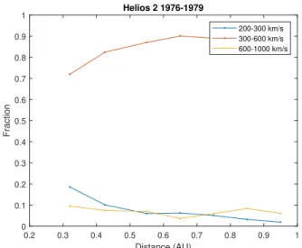
Solar Probe (Bale et al. 2019; Kasper et al. 2019) shows that slow wind can originate in small, equatorial coronal holes; such wind shares several properties with faster, coronal hole wind, such as the pervasive presence of Alfvénic fluctuations. Such slow streams can exist well away from the heliospheric current sheet (HCS); those near the HCS could originate elsewhere, such as at the edges of coronal holes (Wang 2017), intermittent release from the top of helmet streamers, pseudostreamers (Wang et al. 2012), or even from active regions. The very slowest wind is only present close to the Sun (see Fig.1); at larger distances its absence is due either to its continuous acceleration, or its interac-tion with faster surrounding wind. Solar Orbiter, travelling close enough to measure the pristine slow wind before stream–stream interactions destroy the fine-scale structure, will provide new measurements of the plasma and magnetic field in such streams, and, using remote sensing data, the regions from which it originates.
As the solar wind travels anti-Sunward, stream–stream inter-actions develop, ultimately leading to corotating interaction regions (CIRs,Gosling & Pizzo 1999) which can have signifi-cant space weather impacts at the Earth due to their enhanced and complex magnetic field structure (Luan et al. 2013). By compressing the magnetic field into planar magnetic structures (Jones & Balogh 2000), CIRs also impede the propagation of energetic particles; conversely, shocks associated with the stream interactions can also accelerate thermal particles to higher ener-gies. Solar Orbiter will measure the development of CIRs out to 1 AU, as well as their latitudinal dependence.
Ultimately, the IMF reflects the global solar magnetic field driven by its internal dynamo. The evolution of this field over the approximately eleven-year solar cycle, from dipolar near solar minimum, through a complex reversal at maximum, to a new minimum with the opposite polarity, is the direct manifes-tation of dynamics in the solar interior – the dramatic weak-ening of the last two solar maxima, resulting in much weaker solar and interplanetary magnetic fields and even a weaker solar wind flow, highlights the importance of diagnosing and understanding the solar interior. Solar Orbiter’s PHI instrument (Solanki et al. 2020) will remotely measure the solar surface field, and in combination with MAG will map the connections between the solar and interplanetary fields. The evolution of the spacecraft orbit to latitudes over 30◦ by the end of the mission will make it possible to remotely measure the polar fields and directly measure their interplanetary manifestation well above the low-latitude streamer belt. In contrast, Parker Solar Probe, like the Helios spacecraft before it, orbits close to the solar equa-tor. Ulysses (e.g.Smith et al. 2003) travelled to over 80◦ helio-graphic latitude, but with a five-year orbital period could only sample the latitudinal structure of the IMF twice per solar cycle. Solar Orbiter will make repeated measurements of the latitudinal
0.2 0.3 0.4 0.5 0.6 0.7 0.8 0.9 1 Distance (AU) 0 0.1 0.2 0.3 0.4 0.5 0.6 0.7 0.8 0.9 1 Fraction Helios 2 1976-1979 200-300 km/s 300-600 km/s 600-1000 km/s
Fig. 1.Fractional occurrence of hourly averaged speeds measured by Helios 2. The very slowest speeds only occur close to the Sun.
structure of the IMF, and by extension the solar magnetic field, over the evolution of the next solar cycle.
The magnetometer (MAG) instrument will measure the structure of coronal mass ejections (CMEs) and, in conjunc-tion with other missions, their evoluconjunc-tion as they propagate anti-sunward. The magnetic flux associated with CMEs is impli-cated in the evolution of the dynamo over the solar cycle (e.g. Owens & Crooker 2006); near-Sun measurements by MAG will clarify the role of CMEs in the development of the global solar field as well as the fraction of solar magnetic flux open into space as a function of distance, latitude, and phase of the solar cycle. 2.2. Heating and acceleration of the corona and solar wind The solar wind presents a unique laboratory for studying fun-damental plasma processes such as shocks, turbulence, insta-bilities, and reconnection which occur throughout the Universe. These processes are also implicated in the heating of the solar corona and acceleration of the solar wind itself. Solar Orbiter, as it travels close to the Sun with a comprehensive field and plasma payload along with remote sensing instruments to determine the solar source conditions, will provide new and unique measure-ments over a broad range of distances and latitudes.
Non-Maxwellian plasma populations and temperature anisotropies (e.g. Matteini et al. 2007; Chen et al. 2016) can drive instabilities which heat the plasma and drive waves and other fluctuations. Magnetic field measurements from MAG will diagnose such fluctuations and their energy content.
Recent evidence of intermittent Alfvénic velocity spikes (Kasper et al. 2019;Bale et al. 2019; Horbury et al. 2018) sug-gests that reconnection can play a role in heating and driving the solar wind. Solar Orbiter will provide new measurements of these short spikes and characterise their structure, as well as their radial evolution and contribution to the total solar wind energy and momentum budget. Importantly, Solar Orbiter’s near-corotation will make it possible to determine the spatial variation of these structures and link this to their solar origins, in a way which is not possible from near Earth.
Magnetic field measurements are the highest-precision diag-nostic available for turbulence on both fluid and kinetic scales, and can also be used to characterise the dissipa-tion processes that ultimately heat the plasma. Solar Orbiter’s
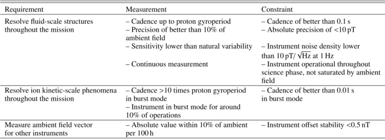
Table 1. MAG performance requirements, including measurement requirements and constraints.
Requirement Measurement Constraint
Resolve fluid-scale structures – Cadence up to proton gyroperiod – Cadence of better than 0.1 s throughout the mission – Precision of better than 10% of – Absolute precision of <10 pT
ambient field
– Sensitivity lower than natural variability – Instrument noise density lower than 10 pT/√Hz at 1 Hz
– Continuous measurement – Instrument operational throughout science phase, not saturated by ambient field
Resolve ion kinetic-scale phenomena – Cadence >10 times proton gyroperiod – Cadence of better than 0.01 s
throughout the mission in burst mode in burst mode
– Instrument in burst mode for around 10% of operations
Measure ambient field vector – Absolute value within 10% of ambient – Instrument offset stability <0.5 nT for other instruments per 100 h
measurements of the near-Sun, dynamically young, turbulent cascade (Bruno & Carbone 2013) will answer several open ques-tions regarding the nature of the cascade and its evolution, par-ticularly in the absence of strong driving and over a wide range of plasma parameters.
MAG will provide high-precision measurements of shock waves throughout the inner heliosphere, and with its triggered burst mode (see Sect.6.2) will measure the fluctuations within and around the shock with a resolution sufficient to resolve sub-ion phenomena.
2.3. Acceleration and propagation of energetic particles The acceleration of particles to high energies and their propaga-tion into the heliosphere, with some arriving in near-Earth space, is not only a fundamental physical process of broad interest, but is also of importance for the survival of space-based tech-nology and indeed astronauts (e.g. Eastwood 2008). The EPD instrument on Solar Orbiter (Rodríguez-Pacheco et al. 2020) will characterise the local energetic particle population, but MAG will play a key role in determining both their acceleration mechanisms and propagation mechanisms. By the time they reach 1 AU, energetic particles have typically scattered and their signatures can be diffuse and difficult to link to acceleration sites. MAG will characterise the acceleration mechanisms, for example properties of near-Sun shocks associated with CMEs, as well as determining the fine-scale structure of the magnetic field which determines the propagation and scattering of the parti-cles, resulting in “particle channels”. MAG will also characterise the development of planar magnetic structures (e.g.Jones et al. 2002) associated with CIRs and CMEs, which can result in For-bush decreases (e.g.Shaikh et al. 2018) of galactic cosmic rays. 2.4. Instrument requirements
Given the overall science goals described above, a set of mea-surement requirements was derived at the beginning of instru-ment developinstru-ment. The MAG instruinstru-ment must:
1. operate continuously throughout the scientific phase of the mission;
2. measure the magnetic field on fluid timescales at all times; 3. for shorter intervals, measure the magnetic field on ion kinetic timescales;
4. measure the field with sufficient resolution and sensitiv-ity to resolve physical phenomena on the relevant measurement timescales; and
5. provide magnetic field measurements in real time to the Radio and Plasma Wave (RPW) and Solar Wind Analyser (SWA) instruments.
These, in combination with expected conditions along the orbit, in turn result in quantitative requirements on the instru-ment, as shown in Table1. As we discuss later in this paper, the Solar Orbiter magnetometer satisfies all these requirements.
The instrument must have sufficient range to measure all amplitudes of fields expected in operation, and in addition, to enable ground operations, the instrument must not saturate in the Earth’s field. This, combined with the finite number of e ffec-tive bits of measurement and the need to resolve the sensor noise floor (under 10 pT) when the field is sufficiently low, leads to a design with several “ranges” of measurement, as is common in space magnetometers. The most sensitive range, that of ±128 nT, has a resolution of around 4 pT. Helios measurements of the heliospheric magnetic field (Fig.2) rarely found field strengths over 100 nT, and therefore the Solar Orbiter magnetometer is expected to remain in its most sensitive range for the vast major-ity of the mission; see Sect.6.
We note that while the average strength of the interplan-etary magnetic field varies with the solar cycle, it decreased significantly during the minimum in 2008 (Wang et al. 2009) and has not recovered back to values seen early in the Space Age: the solar wind density is also lower on average. As a result, the predictions that were made for the original instru-ment proposal in 2008 of the magnetic field strength and several parameters that depend on it (Alfvén speed, particle gyroradii, plasma β), which drove the instrument measurement require-ments, are out of date. Unless the solar wind recovers to its state in the Helios era, Solar Orbiter will experience a rather dif-ferent environment from that experienced by Helios, but MAG still has ample sensitivity and resolution to achieve its science goals.
In addition to placing requirements on the MAG instru-ment, the need to accurately measure the IMF without interfer-ence from artificial signals places stringent requirements on the magnetic fields generated by both the spacecraft and the other instruments. The programme undertaken to achieve these requirements is described in Sect.5.
0.2 0.3 0.4 0.5 0.6 0.7 0.8 0.9 1 Distance (AU) 100 101 102 |B| (nT) Helios 2 1976-1979
Fig. 2. Hourly averaged magnetic field magnitudes measured by Helios 2.
2.5. Collaboration with other instruments
With ten instruments onboard, Solar Orbiter’s science will be maximised by the coordination of observations – indeed, the sci-entific objectives of the mission cannot be achieved without such coordination, including that between the remote sensing and in situ instruments (see Sect.6). Coordination will also take place between various in situ instruments. MAG will provide real time data to RPW and SWA (Sect.6.4) and in turn respond to shock triggers from RPW. Scheduled burst mode intervals will be coor-dinated between the in situ teams as needed to achieve relevant science objectives (Walsh et al. 2020).
It is also planned to merge the MAG and RPW search coil data into one data product, taking into account the better low-frequency response of fluxgates and better high-frequency response of search coils, as has been performed on other spacecraft (e.g. Fischer et al. 2016). Ground measurements are planned with engineering models of MAG and RPW to verify the spectral transfer functions of both instruments in order to optimise this merging process. Since the RPW search coil will record time series only for limited periods, this merged product will not be available throughout the mission.
2.6. Collaboration with other missions
Solar Orbiter will form part of a constellation of spacecraft char-acterising the Sun and inner heliosphere operating in conjunc-tion with Earth-based telescopes. As well as multiple near-Earth telescopic missions such as the Solar Dynamics Observatory and HINODE, in situ measurements will be made by spacecraft near L1, by BepiColombo during its cruise and after arrival at Mercury, by STEREO A and perhaps most notably by Parker Solar Probe (Fox et al. 2016); see Velli et al. (2020). Science planning for MAG operations takes into account the locations of other spacecraft, for example targeting burst mode intervals during a radial line-up with Parker Solar Probe in late 2020.
3. Instrument design
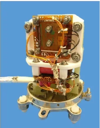
The Solar Orbiter magnetometer (Fig.3) is a conventional dual fluxgate design. Two sensors have been provided and they are accommodated on the spacecraft boom (Fig.4; for details of the spacecraft see García Marirrodriga et al. 2020): MAG-IBS and
Fig. 3.Solar Orbiter flight hardware magnetometer sensors and elec-tronics box.
Fig. 4.Solar Orbiter spacecraft with MAG sensors marked.
MAG-OBS. A dual sensor configuration provides redundancy, and, as they are at different distances (approx. 1 m for IBS and 3 m for OBS) from the spacecraft body, also allows “gradiome-ter” magnetometer characterisation of spacecraft signals in flight (Neubauer & Schatten 1974). The sensors are connected by an electrical harness, along which analogue signals travel to the MAG electronics box (ELB), which houses the following elec-tronics cards:
1. one front end electronics (FEE) card for each sensor, con-taining the sensor drive and field extraction electronics;
2. cold redundant power converter units (PCU), including a DC-DC converter to supply the required secondary voltages and a DC-AC sensor heater supply; and
3. a single instrument controller unit (ICU) which provides redundant SpaceWire data interfaces between the spacecraft and sensors.
Triple redundant thermistors mounted on each sensor block are routed directly to the spacecraft for conditioning and read out via spacecraft housekeeping data, providing sensor tem-perature data when the instrument is both operational and
Table 2. MAG instrument resources.
Unit Mass (g)
Sensor (each) 500
Sensor thermal blanket (each) 55
Electronics box 2200
Sensor harness (each MEP only) 110
Total 3530
Unit Power (W)
Instrument without heaters 7.2
Sensor heaters 5.3
Notes. This table details the elements delivered by the MAG team. The harness running along the boom from the boom root to the sensors them-selves was supplied by the boom contractor, and was ∼125 g m−1.
non-operational. The resource requirements for the instrument are summarised in Table2. A block diagram of the instrument is shown in Fig.5.
3.1. Fluxgate sensors
The fluxgate principle (e.g.Acuña 2002) is well established as a robust, low-power, low-mass magnetometer with high precision and stability. The MAG sensor core design used on Solar Orbiter is essentially identical to those on Double Star (Carr et al. 2005) and Cassini (Dougherty et al. 2004), with two soft magnetic cores procured from Ultra Electronics mounted in a rigid Macor ceramic block to maintain their relative orthogonal orientation. There are also two small printed circuit boards (PCBs) which contain tuning capacitors, redundant thermistors, and electrical connections between the cores and harness. The sensor with its cover removed is shown in Fig.6.
Early in the project, it was anticipated that the thermal and mechanical design from earlier missions – with the ceramic block mounted onto an aluminium baseplate directly attached to the spacecraft boom – could not be used for Solar Orbiter. The addition of strong thermal and mechanical requirements made it impossible to use the earlier design and required significant additional developments.
Solar Orbiter is a three axis stabilised spacecraft with a heat shield on the Sun-pointing face. The two MAG sensors are accommodated on a boom which deploys into shadow on the anti-Sun face. The sensors remain in shadow throughout the mission, apart from offpointing events associated with orbit cor-rections and Venus and Earth gravity assist manoeuvres. With a design requirement to operate with a boom interface temperature of as low as −190◦C and no incident sunlight, the legacy design, without power hungry heaters, would be far too cold to operate and so an extensive re-design programme was instigated. The principal element is a glass-fibre insulating standoff, which acts to thermally isolate the Macor block and cores from the boom mount. The aluminium base plate has been replaced with tita-nium to provide a thermal match to the titatita-nium boom bracket; analyses indicate that with the aluminium sensor cover and MLI insulation the dominant heat loss in flight will be via the electri-cal harness.
The sensor has been qualified for operation to −100◦C. Dual
redundant non-magnetic heaters have been added to the core PCBs for both survival and operation. While uncertainties in the sensor temperatures in flight are still significant, it is hoped that for large parts of the science orbit, the sensor power dissipation will be adequate to maintain the sensors above −100◦C without
heater operation, improving the temperature stability and there-fore reducing offset drift. Heater operation is controlled by the spacecraft, which monitors sensor thermistors for both survival and operation and turns heaters on and off on one-minute bound-aries as required.
During Venus flybys, the sensors and boom will receive both solar and venusian illumination and the sensor is likely to warm well above its usual operating temperature of −90◦C. Careful design of the boom interface bracket and matching of mate-rial (titanium) on both boom and sensor brackets minimises the effects of thermal expansion and should ensure consistent sensor alignment.
Solar Orbiter is a modestly sized spacecraft mounted on a large launcher. Boom vibration levels are therefore signifi-cant, particularly since MAG-OBS is midway along a boom seg-ment. The combination of materials in the sensor housing driven by thermal considerations, with rigid Macor and more flexible glass-fibre, resulted in a failure under test of an early test model. Following extensive structural modelling, small changes to the design resulted in a successful qualification and the Orbiter mag-netometer design (Fig.6) is robust to vibration up to 22 g rms and a very broad temperature range −100◦C to+45◦C; with a total sensor mass of 500 g, including housing, 30 cm harness, and con-nector, this represents a robust design for many future scientific applications.
3.2. Front end electronics (FEE)
The Solar Orbiter FEE design is a digital implementation of the analogue design flown on the Double Star mission (Carr et al. 2005). A 15.35 kHz drive signal (F) is imposed on two toroidal, orthogonal fluxgate cores using a toroidal drive winding to force periodic saturation. The presence of an ambient field results in asymmetry in the saturation, causing a hysteresis which can be detected as a harmonic of the drive signal in sense coils wound as a solenoid pick up coil around each core. The sense coils detect the field proportional signal at twice the drive frequency (2F, 30.72 kHz) and are also used to supply a feedback current to exactly negate the measured field in the DC–500 Hz range. Such a closed loop configuration improves linearity, with the ampli-tude and direction of the applied nulling current proportional to the ambient field. Each core is wrapped with two orthogo-nal sense windings, providing a three-axis measurement across two cores. One axis (sensor Y axis) is sensed by both cores: these two sense windings are connected in series and routed to single-sense electronics. Thus, the field is completely nulled out in each of the sensor cores, reducing cross talk between axes.
On the FEE card, the sense signals are tuned to provide amplification of the 2F sensor signal, passed through an addi-tion amplifier, and then immediately digitised via a 14-bit analogue-to-digital converter (ADC) operating at 64 times the drive frequency. The ADC signal is passed to an RTAX field-programmable gate array (FPGA). A bandpass filter is applied to the digitised sense signal within the FPGA to generate the field proportional signal, which is integrated and fed to a sigma delta digital-to-analogue converter (DAC) partially embedded in the FPGA (O’Brien et al. 2007) to generate the required feedback current. The output of the DAC from the FPGA is passed through an analogue low pass filter (Butterworth, third order, cut-off fre-quency 500 Hz) and then a voltage to current converter before being fed back to the feedback coil via a 2F blocking circuit to avoid contamination of the incoming sense signal. The field proportional signal from each axis is additionally fed to a dig-ital third-order low pass cascaded integration comb (CIC) filter
Fig. 5.Solar Orbiter magnetometer functional diagram.
(Hogenauer 1981) before being passed from the front-end elec-tronics to the MAG instrument controller unit in blocks of 28 vectors at 1920 Hz via an SPI interface.
3.3. Power control unit (PCU)
The PCU is a custom implementation designed at Imperial Col-lege London, building on heritage from Venus Express and Bepi Colombo. It provides the required secondary voltages (±8 V, 3.3 V, 2.5 V, 1.8 V and 1.5 V) for the ICU and FEE boards from the input spacecraft 28 V line, and a sensor heater DC-AC con-verter to supply a sensor heating supply at 262 kHz from a sep-arate spacecraft 28 V heater line. The AC heater signal is routed to redundant non-magnetic heater mats fitted to the sensor block. There is a single heater line supplying current to the heater mats on both the OBS and IBS sensors; these can only be operated together. The heaters are operated based on thresholds (update-able by telecommand) of the OBS sensor temperature. The OBS sensor, being further from the spacecraft, will experience lower temperatures to the IBS sensor.
3.4. Instrument controller unit (ICU)
The ICU hosts a Central Processing Unit (CPU) based on a custom version of the 25 MHz Leon3FT-RTAX PC1 configura-tion provided by Aeroflex Gaisler, hosted on a RTAX2000S/SL FPGA. The RTAX configuration is bespoke for Imperial College London, with additional IP: two SpaceWire cores; two SPI cores for communication with the sensor FEEs; a SPI core for com-munication with housekeeping ADCs; a debug support unit; a UART serial link; a CCSDS Time Manager; and a memory con-troller. The Leon3FT is fault tolerant and supports memory error detection and correction (EDAC).
The ICU has four 32Kx8 programmable read only memory (PROM) chips which hold a copy of the boot software (BSW), a
Fig. 6.Solar Orbiter magnetometer sensor, without cover, showing the two cores, heater pads and associated wiring.
256Kx32 electronically erasable programmable read only mem-ory (EEPROM) which holds three instances of the application software (ASW), and a 1Mx39 static random access memory
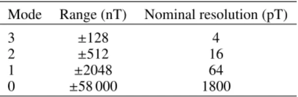
Table 3. Magnetometer resolution for the four operating ranges.
Mode Range (nT) Nominal resolution (pT)
3 ±128 4
2 ±512 16
1 ±2048 64
0 ±58 000 1800
Notes. All three axes of each sensor will be in the same range. OBS and IBS can operate in different ranges. Range can be changed via telecom-mand, or autonomously by the instrument in response to the measured field.
(SRAM). In science operation, most of the SRAM is used for rolling burst-mode buffers (see Sect.6.2). The ICU performs the following functions:
1. Data interfacing to the spacecraft via dual 10 MHz SpaceWire connections, including processing and responding to telecommands and generating telemetry packets;
2. monitoring of instrument health via measurement at 8 Hz of secondary voltages and electronics temperature, and send-ing warnsend-ing and danger events to the spacecraft should these parameters exceed defined thresholds. The ICU houses redun-dant housekeeping ADCs which digitise the secondary voltages and transmit these to the processor;
3. generation of event packets in response to instrument mode changes, and to indicate reception and execution status of telecommands;
4. decimation and filtering of the 1920 vectors/s data streams from the two sensor FEE boards into appropriate data prod-ucts depending on instrument mode, including timestamping. The incoming 1920 Hz data are low pass filtered and decimated via a second-order CIC operating in the ICU to produce the required data rates for normal and burst modes, with an indepen-dent filter working for each sensor and each data stream. This produces 128 Hz burst mode data with a bandwidth of approxi-mately 10 Hz;
5. range control of the sensors, both via command and autonomously detecting when all three components are below a threshold of 12.5% full scale, and commanding the FEE into a more sensitive range. The FEE will autonomously up-range to a less sensitive range if any axis exceeds 87.5% of full scale to avoid saturation of the sense signal ADCs. Ranges are given in Table3; 6. detection of burst mode triggers, and changing the instru-ment mode as appropriate based on content of inter-instruinstru-ment communication packets;
7. application of a calibration matrix to the measured data for onboard distribution to the SWA and RPW instruments; and
8. patching of flight software on the EEPROM.
Early in development of the MAG software, a decision was made to undertake common development of the BSW and ASW. A real-time operating system was required and RTEMS v4.10 was selected for its robustness and availability of drivers including SpaceWire. The MAG instrument boots into the BSW which is held in PROM and is non-patchable. Boot software does not allow science operations but can support in-flight patching of application software in EEPROM. Following extensive devel-opment effort, a very flexible patching capability is available, with blank areas of memory interspersed within the ASW code to allow the uploading of small updates to individual subroutines as required.
Typical operation of MAG will entail power-on, entry to BSW, and then a rapid, commanded transition to ASW. In ASW, the sensors will be activated (by pulling the front-end
electron-Table 4. Magnetometer data streams.
Data stream Primary Secondary (samples/s) (samples/s)
Low latency 0.125 None
Normal (N) 16 1 Normal (L) 1 1 Normal (E8) 8 8 Burst (B) 128 8 Burst (B64) 64 8 Burst (B128) 128 128 Engineering 1920 None
Notes. Science mode is either “normal” where low latency and one of the three normal mode data streams will be produced, or “burst”, where low latency, one of the normal mode data streams and one of the three burst mode streams will be produced. An engineering data stream at 1920 Hz from the primary sensor can also be produced, although this is only anticipated to be used for short periods during commissioning.
ics FPGAs out of reset) with the ICU autonomously monitoring the activation status to ensure successful initiation of the reso-nant sensor drive circuit. It is expected that following successful entry into science operations, the MAG instrument will remain operating in this mode for months, and ideally years, without turning off. The current longest duration test is over 6 weeks, demonstrating that the software is robust to continuous unsup-ported operation.
4. Instrument performance
The magnetic field in interplanetary space at 1 au is around five orders of magnitude smaller than that at the Earth’s sur-face, with fluctuations on proton gyroscales nearly three orders smaller still. The characterisation of magnetometers on the ground before flight is therefore challenging and specialist facil-ities are required.
To provide a representative, low-field, low-noise magnetic field environment for sensor test and verification, the sensors were tested within mu-metal shields: Imperial College London has a five-layer shield that operates at room temperature and a three-layer shield with thermal control system that allows the sensor to be cooled with nitrogen down to −150◦C. In both
shields, the field is reduced to just a few nanoTesla with noise levels below the noise floor of the instrument at 10 pT Hz−1/2at
1 Hz, despite the challenging magnetic environment in central London.
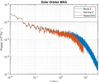
Particular attention was paid during the electronics design and development from lab model to engineering and qualifica-tion models to reduce the electronics noise, resulting in the clean spectra as shown in Fig.7, well below the 10 pT Hz−1/2at 1 Hz requirement. The high-frequency roll-off of the spectrum due to the anti-aliasing filter is also clear in the spectrum.
While the dynamic electrical environment in the Imperial College lab means that the magnetic field even in shielding cans typically shows variations of order 0.5 nT over a day, the flight instrument showed excellent stability over several days during ground operation (Fig.8).
5. Magnetic cleanliness
Two factors mean that the MAG sensors are considerably closer to the spacecraft body than is desirable from an electromagnetic
10-2 10-1 100 101 f (Hz) 10-7 10-6 10-5 10-4 10-3 Power (nT 2Hz -1)
Solar Orbiter MAG
Burst Z Normal Z Noise limit
Fig. 7.Power spectra of normal and burst-mode data from the Solar Orbiter magnetometer flight model outboard sensor, operating in the most sensitive range. A single axis is shown. The 10 pT Hz−1/2at 1 Hz
noise requirement is marked for reference.
-1 -0.5 0 0.5 1 X (nT)
Solar Orbiter MAG (means removed)
-1 -0.5 0 0.5 1 Y (nT) 306 21 00 307 00 00 307 03 00 307 06 00 307 09 00 2009, dayno hour min (UT)
-1 -0.5 0 0.5 1 Z (nT)
Fig. 8.Magnetometer data (means removed) taken within a magnetic shielding can at Imperial College London. Drifts over the >12 h interval are typical of local variations rather than sensor offsets.
compatibility (EMC) perspective: physical constraints of the spacecraft body size, meaning that the two-hinge boom is rather short; and a desire to enhance the field of view of the SWA/EAS electron sensor (Owen et al. 2020) resulting in this sensor being placed at the boom end.
The need to measure magnetic field fluctuations on kinetic scales, with amplitudes down to 10 pT, requires a very quiet magnetic environment at the outboard sensor location. It was considered unrealistic, given the complex remote sensing instru-ments and relatively short boom, to place an overall magnetic requirement at this level. Therefore, a comprehensive magnetic cleanliness programme (requiring support from the prime con-tractor, ESA, and all the instrument teams) has been undertaken, and the concept of EMC quiet periods for the mission has been introduced. The mission is required to be EMC quiet for at least 70% of the science orbit, in periods of at least 1 h. Known noisy activities such as solar array movements and reaction wheel o ff-loadings will be coordinated as far as possible and EMC noisy periods identified, with instrument noisy activities ideally also
placed in these intervals. All spacecraft-controlled heaters will be powered up or down on one-minute boundaries, with their operation reported in telemetry to allow their magnetic signature to be removed from the MAG data.
During EMC quiet periods, any AC signals below 64 Hz (i.e. the burst mode Nyquist frequency) as measured at the OBS loca-tion are required to either be below the noise floor of the OBS sensor (<10 pT), that is, invisible to the MAG instrument, or to be transients, superimposed on the DC value, (including step functions) of <1 s duration and <1 nT amplitude at the OBS sen-sor, which can be identified by events reported in telemetry, that is, signals which can be easily removed from the MAG data.
The magnetic performance of all instruments and spacecraft units were verified at unit level prior to delivery, scaling the mea-sured unit-generated signals to an equivalent unit-OBS distance, with results presented and discussed at project EMC working group meetings. At these meetings, a classification was made for all instrument modes and events as either EMC quiet (and therefore allowed during EMC quiet periods) or EMC noisy (and therefore to be confined to non-EMC quiet parts of the orbit). A final characterisation of the almost fully integrated spacecraft was performed at the MFSA magnetic test facility at IABG in Munich. During this test, the unpowered spacecraft was moved on a non-magnetic trolley through a ring of eight mag-netometers, with an additional three magnetometers located at the deployed boom locations for IBS, OBS, and the AC magne-tometer in an Earth’s field compensation coil system to verify the DC magnetic requirement at the OBS sensor location. The MAG sensors themselves were located on the stowed boom on the SC for the test (the spacecraft with deployed boom would not fit inside the facility). Following this unpowered test, a powered test was completed, with the stationary spacecraft configured to an EMC-quiet operational state to confirm the DC contamina-tion was below requirements. A second day of characterisacontamina-tion of a prioritised subset of spacecraft and instrument unit mag-netic performance was also carried out to further verify EMC quiet classification.
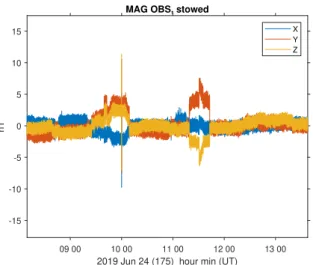
This testing, although limited due to schedule constraints to just one day of unpowered and two days powered testing, has provided a wealth of magnetic field characterisation data which will be invaluable for distinguishing real from spacecraft-generated signals in space; an example is shown in Fig. 9. Importantly, many signals are well correlated with instruments’ current consumption, meaning that with this data, the signals could potentially be removed. Further analysis will be performed on magnetic field data recorded during spacecraft and instrument commissioning activities.
6. Operations concept
The operational principle of the MAG instrument is straightfor-ward and has been designed to require minimal maintenance and operator input. MAG is expected to operate continuously throughout the cruise, science, and extended phases of the mis-sion and emphasis has therefore been placed on simplicity of the operational strategy. Key operational tasks, beyond health mon-itoring and maintenance, are expected to be the coordination of burst modes with other instruments and the on-ground calibra-tion of the received data.
The instrument has four ranges (Table 3), and will autonomously switch between them to ensure high-resolution without saturation. If the field in any axis of a sensor exceeds 87.5% of the amplitude of the existing range, all three axes of that sensor will move to the next range. If the field in all three
09 00 10 00 11 00 12 00 13 00
2019 Jun 24 (175) hour min (UT)
-15 -10 -5 0 5 10 15 nT
MAG OBS, stowed
X Y Z
Fig. 9.MAG OBS time series from spacecraft-level magnetic field char-acterisation testing, showing DC level shifts and spikes associated with the operation of other instruments. These measurements were taken with the boom stowed, meaning that the MAG sensor was much closer to the spacecraft than will be the case in flight.
axes remains below 12.5% of the current range for more than a configurable time (nominally 10 s) then the sensor will drop into the next most sensitive range. Due to spacecraft fields at the IBS location, it is expected to be routinely in Range 2, whilst OBS should routinely operate in the most sensitive range, Range 3, apart from during the strongest fields near perihelion.
MAG has several science operational modes (Table4) which represent different cadence data from the primary (nominally outboard, OBS) and secondary (nominally inboard IBS) sensors. 6.1. Normal mode
Based on experience from earlier missions such as Ulysses and Cluster, the highest scientific priority is a continuous, homoge-neous dataset at a cadence sufficient to resolve up to the pro-ton gyroscale: this cadence has been selected at 16 vectors/s for the outboard sensor. The inboard sensor will return 1 vector/s to allow gradiometer mode assessment of spacecraft magnetic field perturbations. An “Equal8” mode where both sensors return 8 vectors/s is available: this will be used if spacecraft field vari-ations are so rapid that a gradiometer mode is required to be run continually. This is not expected to be the case.
During cruise phase, telemetry allocations are expected to be lower than for normal science operations for several months, and in order to ensure continuous data coverage a low rate nor-mal mode at 1 vector/s cadence from each sensor has also been implemented.
6.2. Burst mode
Higher cadence than normal mode is required to reach below the proton gyroscale. A burst mode of 128 vectors/s from the primary sensor has been implemented, which within the teleme-try allocation will allow around 1 h per day of burst data. As it is expected that the natural signal will be below the MAG sensor noise floor above around 10 Hz, a further burst mode (“Burst64”) of 64 vectors/s was implemented, allowing around 2 h/day of coverage, and this is expected to be used routinely, with higher rate burst modes only used for engineering pur-poses. An additional burst mode which provides 128 vectors/s
from both primary and secondary sensors will be used during the boom deployment and for periods of commissioning to help characterise the magnetic field of the spacecraft. An engineering mode can also be enabled, which produces 1920 vector/s data from the primary sensor. These higher data rate modes will be used in commissioning to verify instrument performance, but the limited telemetry rates mean that they will rarely if ever be used in flight.
The modest normal mode data rate achieved by MAG means that its burst mode can run for significantly longer each day, on average, than other in situ instruments. The operational strategy for burst mode is to coordinate with other in situ instruments and enter burst mode whenever any other instrument is in burst mode, as well as command burst mode intervals, probably in blocks of 30 min, as the telemetry allocation allows. Burst mode can be triggered by timed telecommand or by receipt of the RPW real time shock trigger via onboard packets on the SpaceWire link; in future, an internal MAG trigger could be implemented.
The RPW shock algorithm does not immediately detect a shock and there is also scientific interest in the region imme-diately upstream of the shock. A rolling buffer, holding 6 min of burst mode data, has therefore been implemented and this will be emptied into the spacecraft solid state mass memory (SSMM) whenever a burst mode is triggered or commanded.
Traditionally, instruments are either in normal or burst mode, however this can potentially result in gaps in the data return: since the number of burst triggers is unknown beforehand, it is possible that more burst-mode intervals will be recorded than can fit in the store or be telemetered to ground. If no normal-mode data were taken during burst normal-mode intervals, there would be gaps in the final data stream. As a result, MAG continues to produce normal-mode data even when in burst mode. Burst-mode and normal-Burst-mode data are routed to different packet stores on the spacecraft SSMM, so even if the burst-mode store is filled, a continuous normal-mode data stream will be brought down to ground.
The MAG team will select burst-mode intervals to coordinate with other instrument teams, especially the in situ instruments. The strategy for determining commanded burst-mode intervals has not been finalised but it is likely that MAG will take at least 30 min of continuous burst mode data every day during the sci-ence phase of the mission. As a result of this strategy, the MAG instrument internally generates four main data streams (normal and burst for both sensors) continually, with digital low pass fil-ters appropriate to the cadence selected and implemented in the ICU.
6.3. Low-latency data
Depending on the downlink rate, normal- and burst-mode data can remain on the spacecraft for months before transmission to Earth. The MAG instrument generates a low-data-rate product which will be downlinked at every pass to allow mission-level short-term planning decisions to be made, for example by reveal-ing whether the heliospheric current sheet has been crossed. This “low-latency” data stream is plucked from the outboard sensor normal-mode stream once every 8 s and therefore does not have cadence-specific filtering applied. Removal of the offsets from this data stream will be challenging and it is not expected to ever be of science quality.
6.4. Inter-instrument communication
The SWA and RPW instruments require magnetic field data in real time. SWA uses the magnetic field unit vector to generate
rapid reduced distribution functions (Owen et al. 2020) while RPW uses the magnetic field magnitude as an input to its shock-detection algorithm (Maksimovic et al. 2020). MAG distributes these data on the SpaceWire link via “service 20” packets which are sent eight times per second, a cadence which is driven by the SWA requirement.
The MAG service 20 packets provide magnetic field vectors in the spacecraft frame, in nanoTesla. It is therefore necessary for the instrument to apply a calibration matrix in real time, both rotating the vector from sensor coordinates and removing space-craft magnetic fields. This is performed in fixed point arithmetic using an uploaded calibration matrix and a resolution of around 0.1 nT. At this time, it is not clear how variable the spacecraft fields will be and how often a new calibration matrix can be cal-culated and uploaded, and so the ultimate precision of the real-time MAG vectors is not likely to be known until flight. 6.5. Operations planning
Successful science operation of Solar Orbiter requires coordi-nated observations from both remote sensing and in situ instru-ments, taking into account the overall mission goals, spacecraft orbit, and telemetry constraints (Zouganelis et al. 2020). Science coordination is undertaken within the framework of the Sci-ence Operations Working Group (SOWG; see Sanchez et al., in prep.). Within that agreed overall mission profile, MAG opera-tions will be planned 6 months ahead of execution, in blocks of 6 months of operations, covering roughly one orbit. The MAG planning is relatively straightforward and will consist of coordi-nating burst mode intervals to maximise the science return taking into account:
1. coordinated burst mode intervals with other Solar Orbiter instruments;
2. data rates during EMC quiet and noisy periods;
3. conjunctions with other spacecraft, such as Parker Solar Probe, Bepi Colombo, and Stereo; and
4. balancing normal- and burst-mode acquisition with the telemetry allocation for the MAG instrument, which varies con-siderably with the orbit.
The In Situ Working Group (Walsh et al. 2020) will also be used as a mechanism for coordinating science between the in situ payload, in terms of both operations planning and exploitation following data return.
6.6. Processing and calibration
The MAG data will be processed into common data format (CDF) data files with increasing levels of calibration applied. Calibration in this sense is used to cover the removal of sensor offsets, and also any cleaning that is required to remove space-craft signatures from the data.
1. Level 0: Raw uncalibrated data for internal use only. 2. Level 1: Un-calibrated data in units of nT in the unit ref-erence frame.
3. Level 2: Calibrated data in RTN coordinates and in the spacecraft reference frame. These data will be released to the community through the archive 90 days after acquisition and will be scientifically useable.
4. Level 3: A subset of Level 2 data with further calibration applied. Likely to be of a higher cadence than Level 2.
The magnetometer underwent a ground calibration at the Magnetsrode facility near Braunschweig (Glassmeier et al. 2007), where offsets, relative orthogonality, and gains were determined for each sensor and every operating range, at both
room temperature and −100◦C, close to the expected operating temperature. These values will be used as the starting point for in-flight calibration.
In-flight calibration will use aHedgecock(1975)-based pro-cedure for data in the solar wind, plus data collected dur-ing spacecraft rolls planned for once per orbit to calculate the spacecraft-generated field at the sensor locations. Pre-flight anal-ysis shows that these fields can be routinely determined to a pre-cision of around 0.1 nT. Sensor relative gain and orthogonality parameters are unlikely to be determined better in flight than from ground calibration, so the latter values are expected to be used throughout the mission.
Several science goals of the MAG team require comparison of the fluxgate data with those of other in situ instruments, where co-alignment knowledge is vital. Boom deployment knowledge will only constrain the MAG sensor orientation to around 1◦
but this can be improved upon by comparison with other sen-sor data. Co-alignment with the RPW search coil magnetome-ter, which is also situated on the boom, will be determined by a covariance analysis of the two data sets. Co-alignment with the SWA/PAS ion sensor will be determined by comparing the symmetry direction of the proton distribution with the instan-taneous field direction measured by MAG. Since PAS is fixed on the spacecraft body, this should also provide more accurate determination of the MAG sensor alignment with the spacecraft reference frame and hence, via spacecraft attitude, a heliospheric coordinate system. Accurate knowledge of the magnetic field direction is important for quantitative studies of the heliospheric flux budget and its evolution over the solar cycle.
6.7. Data distribution
Following calibration, magnetometer data will be distributed via ESA’s Solar Orbiter data archive (Sanchez et al., in prep.). It is a requirement that data be made public 90 days following receipt on the ground; given the possible level of magnetic contamina-tion from the spacecraft and instruments, this is a challenging goal and it is likely that subsequent, improved revisions of the public data will be made available at a later date.
Automatically processed low-latency data (see Sect.6.3) will be made available via ESDC immediately. Although of interest for providing context, these data will not be of science quality, given that they will not have been subject to a full calibration sequence.
7. Conclusions
The Solar Orbiter magnetometer meets all its requirements and is fully qualified, integrated on the spacecraft, and operating as expected. The instrument will play a key role in the increase in understanding of the dynamics of the Sun and heliosphere pro-vided by Solar Orbiter in the coming decade.
Acknowledgements. The Solar Orbiter magnetometer was funded by the UK Space Agency (grant ST/T001062/1). We gratefully acknowledge the work of all the engineers who supported the instrument development but have since left Imperial College as well as the support of the engineering and technical staff at Airbus Space and the European Space Agency during the Solar Orbiter project. Helios data were provided by NASA’s NSSDC. This paper is dedicated to the memory of Trevor Beek, Lawrence Soung Yee and Andy Breen.
References
Acuña, M. H. 2002,Rev. Sci. Instrum., 73, 3717
Bruno, R., & Carbone, V. 2013,Liv. Rev. Sol. Phys., 10, 2
Carr, C., Brown, P., Zhang, T., et al. 2005,Annal. Geophys., 23, 2713
Chen, C. H. K., Matteini, L., Schekochihin, A. A., et al. 2016, ApJ, 825, L26
Cranmer, S. 2002,Space Sci. Rev., 101, 229
D’Amicis, R., Matteini, L., & Bruno, R. 2019,MNRAS, 483, 4665
Dougherty, M. K., Kellock, S., Southwood, D. J., et al. 2004, The Cassini Magnetic Field Investigation(Dordrecht: Springer Netherlands), 331 Eastwood, J. P. 2008,Philos. Trans. R. Soc. A: Math. Phys. Eng. Sci., 366, 4489 Fischer, D., Magnes, W., Hagen, C., et al. 2016,Geosci. Instrum. Meth. Data
Syst., 5, 521
Fox, N., Velli, M., Bale, S., et al. 2016,Space Sci. Rev., 204, 7
García Marirrodriga, C., Pacros, A., Strandmoe, S., et al. 2020, A&A, in press, https://doi.org/10.1051/0004-6361/202038519(Solar Orbiter SI) Glassmeier, K.-H., Richter, I., Diedrich, A., et al. 2007,Space Sci. Rev., 128,
649
Gosling, J. T., & Pizzo, V. J. 1999, inCorotating Interaction Regions, eds. A. Balogh, J. T. Gosling, J. R. Jokipii, R. Kallenbach, & H. Kunow (Dordrecht: Springer Netherlands), 21
Hedgecock, P. C. 1975,Space Sci. Instrum., 1, 83
Hogenauer, E. 1981, IEEE Transactions on Acoustics, Speech, and Signal Processing, 29, 155
Horbury, T. S., Matteini, L., & Stansby, D. 2018,MNRAS, 478, 1980 Jones, G., & Balogh, A. 2000,J. Geophys. Res.: Space Phys., 105, 12713 Jones, G. H., Rees, A., Balogh, A., & Forsyth, R. J. 2002,Geophys. Res. Lett.,
29, 15
Kasper, J. C., Bale, S. D., Belcher, J. W., et al. 2019,Nature, 576, 228 Luan, X., Wang, W., Lei, J., et al. 2013,J. Geophys. Res.: Space Phys., 118, 1255 Maksimovic, M., Bale, S. D., Chust, T., et al. 2020,A&A, 642, A12(Solar
Orbiter SI)
Matteini, L., Landi, S., Hellinger, P., et al. 2007,Geophys. Res. Lett., 34, L20105 Müller, D., Marsden, R. G., St. Cyr, O. C., & Gilbert, H. R. 2013,Sol. Phys.,
285, 25
Müller, D., St. Cyr, O. C., Zouganelis, I., et al. 2020,A&A, 642, A1(Solar Orbiter SI)
Neubauer, F. M., & Schatten, K. H. 1974,J. Geophys. Res. (1896–1977), 79, 1550
O’Brien, H., Brown, P., Beek, T., et al. 2007,Meas. Sci. Technol., 18, 3645 Owens, M. J., & Crooker, N. U. 2006,J. Geophys. Res.: Space Phys., 111, A10 Owens, M. J., & Forsyth, R. J. 2013,Liv. Rev. Sol. Phys., 10, 5
Owen, C. J., Bruno, R., Livi, S., et al. 2020,A&A, 642, A16(Solar Orbiter SI) Rodríguez-Pacheco, J., Wimmer-Schweingruber, R. F., Mason, G. M., et al.
2020,A&A, 642, A7(Solar Obiter SI)
Schwenn, R., & Marsch, E. 1990,Physics of the Inner Heliosphere I: Large-scale Phenomena(Berlin, Heidelberg: Springer-Verlag)
Schwenn, R., & Marsch, E. 1991,Physics of the Inner Heliosphere II. Particles, Waves and Turbulence(Berlin, Heidelberg: Springer-Verlag)
Shaikh, Z. I., Raghav, A. N., Vichare, G., Bhaskar, A., & Mishra, W. 2018,ApJ, 866, 118
Smith, E., Marsden, R., Balogh, A., et al. 2003,Science, 302, 1165
Solanki, S. K., del Toro Iniesta, J. C., Woch, J., et al. 2020,A&A, 642, A11 (Solar Orbiter SI)
Velli, M., Harra, L. K., Vourlidas, A., et al. 2020,A&A, 642, A4(Solar Orbiter SI)
Walsh, A. P., Horbury, T. S., Maksimovic, M., et al. 2020,A&A, 642, A5(Solar Orbiter SI)
Wang, Y.-M. 2017,ApJ, 841, 94
Wang, Y.-M., Robbrecht, E., & Sheeley, N. R. 2009,ApJ, 707, 1372
Wang, Y. M., Grappin, R., Robbrecht, E., & Sheeley, N. R., Jr. 2012,ApJ, 749, 182
Zouganelis, I., De Groof, A., Walsh, A. P., et al. 2020,A&A, 642, A3(Solar Orbiter SI)
1 Imperial College London, South Kensington Campus, London SW7
2AZ, UK
e-mail: [email protected]
2 Evonetix Ltd, Cambridge, UK 3 Arquimea Ingenieria, Madrid, Spain 4 Atomio, Lille, France
5 CERN, Geneva, Switzerland
6 Mullard Space Science Laboratory, University College London,
Holmbury St. Mary, UK
7 School of Physics and Astronomy, Queen Mary University of
London, London E1 4NS, UK
8 SUPA School of Physics and Astronomy, University of Glasgow,
Glasgow G12 8QQ, UK
9 Univ. Reading, Dept. Meteorol., Reading RG6 6BB, Berks, UK 10 Centre for Fusion, Space & Astrophysics, Physics Dept., University
of Warwick, Coventry, UK
11 Jeremiah Horrocks Institute, University of Central Lancashire,
Pre-ston, UK
12 Space Sciences Laboratory, University of California, Berkeley, CA
94720-7450, USA
13 Space Research Institute, Austrian Academy of Sciences, Graz,
Austria
14 University of Calabria, Dipartimento Fis, Arcavacata di Rende,
Cosenza, Italy
15 Wigner RCP, Budapest, Hungary
16 Lunar and Planetary Laboratory, U. Arizona, Tucson, AZ, USA 17 Technical University of Braunschweig, IGEP, Mendelssohnstr. 3,
Braunschweig, Germany
18 University of Maryland Baltimore County, Goddard Planetary
Heliophys Inst., Baltimore, MD, USA
19 Stanford University, Stanford, CA, USA
20 LESIA, Observatoire de Paris, Universite PSL, CNRS, Sorbonne
Universite, Universite de Paris, 5 Pl. Jules Janssen, 92190 Meudon, France
21 Institut für Experimentelle und Angewandte Physik,
Christian-Albrechts-Universität zu Kiel, Kiel, Germany
22 University of Delaware, Newark, DE, USA 23 Universidad de Alcala, Madrid, Spain
24 NASA Jet Propulsion Laboratory, Pasadena, USA 25 Predictive Science Inc., San Diego, CA, USA
26 University of California Los Angeles, Inst. Geophys. & Planetary
Phys., Dept. Earth Planetary & Space Sci., Los Angeles, CA, USA
27 University of Turku, Dept. Phys. & Astron., Turku, Finland 28 Technical University of Denmark, Natl. Space Inst., Copenhagen,
Denmark
29 Center for Space and Aeronomic Research (CSPAR) and
Depart-ment of Space Science, University of Alabama in Huntsville, Huntsville, USA
30 European Space Agency, ESTEC (SCI-S), PO Box 299, Noordwijk
2200 AG, The Netherlands
31 European Space Agency, ESAC (SCI-S), Madrid, Spain 32 University of Colorado, Boulder, CO, USA
33 Physics Department, University of California, Berkeley, CA