HAL Id: insu-01814215
https://hal-insu.archives-ouvertes.fr/insu-01814215
Submitted on 13 Feb 2021HAL is a multi-disciplinary open access archive for the deposit and dissemination of sci-entific research documents, whether they are pub-lished or not. The documents may come from teaching and research institutions in France or abroad, or from public or private research centers.
L’archive ouverte pluridisciplinaire HAL, est destinée au dépôt et à la diffusion de documents scientifiques de niveau recherche, publiés ou non, émanant des établissements d’enseignement et de recherche français ou étrangers, des laboratoires publics ou privés.
Distributed under a Creative Commons Attribution - NonCommercial| 4.0 International License
Generated by Solar Wind Charge Exchange with
Neutrals
David G. Sibeck, R. Allen, Homayon Aryan, Dennis Bodewits, P. Brandt,
Graziella Branduardi-Raymont, G. Brown, Jenny A. Carter, Yaireska
Collado-Vega, Michael R. Collier, et al.
To cite this version:
David G. Sibeck, R. Allen, Homayon Aryan, Dennis Bodewits, P. Brandt, et al.. Imaging Plasma Density Structures in the Soft X-Rays Generated by Solar Wind Charge Exchange with Neutrals. Space Science Reviews, Springer Verlag, 2018, 214, pp.art. 79. �10.1007/s11214-018-0504-7�. �insu-01814215�
https://doi.org/10.1007/s11214-018-0504-7
Imaging Plasma Density Structures in the Soft X-Rays
Generated by Solar Wind Charge Exchange
with Neutrals
David G. Sibeck1· R. Allen2· H. Aryan3· D. Bodewits4· P. Brandt2·
G. Branduardi-Raymont5· G. Brown6· J.A. Carter7· Y.M. Collado-Vega3·
M.R. Collier3· H.K. Connor8· T.E. Cravens9· Y. Ezoe10· M.-C. Fok3· M. Galeazzi11·
O. Gutynska3· M. Holmström12· S.-Y. Hsieh2· K. Ishikawa13· D. Koutroumpa14·
K.D. Kuntz15 · M. Leutenegger3,16· Y. Miyoshi17· F.S. Porter3· M.E. Purucker3·
A.M. Read7· J. Raeder18· I.P. Robertson9· A.A. Samsonov19· S. Sembay7·
S.L. Snowden3· N.E. Thomas3,16· R. von Steiger20· B.M. Walsh21· S. Wing2
Received: 7 December 2017 / Accepted: 3 April 2018 / Published online: 12 June 2018 © The Author(s) 2018
Abstract Both heliophysics and planetary physics seek to understand the complex nature of the solar wind’s interaction with solar system obstacles like Earth’s magnetosphere, the iono-spheres of Venus and Mars, and comets. Studies with this objective are frequently conducted with the help of single or multipoint in situ electromagnetic field and particle observations, guided by the predictions of both local and global numerical simulations, and placed in
con-B
K.D. KuntzD.G. Sibeck
1 Code 674, NASA/GSFC, Greenbelt, MD, USA
2 The Johns Hopkins University Applied Research Laboratory, Laural, MD, USA 3 NASA/Goddard Space Flight Center, Greenbelt, MD, USA
4 University of Maryland College Park, College Park, MD, USA
5 Mullard Space Science Laboratory, University College London, London, UK 6 Lawrence Livermore National Laboratory, Livermore, CA, USA
7 University of Leicester, Leicester, UK 8 University of Alaska, Fairbanks, AK, USA 9 University of Kansas, Lawrence, KS, USA
10 Department of Physics, Tokyo Metropolitan University, Tokyo, Japan 11 University of Miami, Miami, FL, USA
12 Swedish Institute of Space Physics, Kiruna, Sweden
13 JAXA/Institute of Space and Astronautical Science, Sagamihara, Kanagawa, Japan 14 LATMOS/IPSL, UVSQ – Université Paris-Saclay, UPMC – Université Paris 06, CNRS,
Guyancourt, France
text by observations from far and extreme ultraviolet (FUV, EUV), hard X-ray, and energetic neutral atom imagers (ENA). Each proposed interaction mechanism (e.g., steady or transient magnetic reconnection, local or global magnetic reconnection, ion pick-up, or the Kelvin-Helmholtz instability) generates diagnostic plasma density structures. The significance of each mechanism to the overall interaction (as measured in terms of atmospheric/ionospheric loss at comets, Venus, and Mars or global magnetospheric/ionospheric convection at Earth) remains to be determined but can be evaluated on the basis of how often the density sig-natures that it generates are observed as a function of solar wind conditions. This paper reviews efforts to image the diagnostic plasma density structures in the soft (low energy, 0.1–2.0 keV) X-rays produced when high charge state solar wind ions exchange electrons with the exospheric neutrals surrounding solar system obstacles.
The introduction notes that theory, local, and global simulations predict the characteris-tics of plasma boundaries such the bow shock and magnetopause (including location, density gradient, and motion) and regions such as the magnetosheath (including density and width) as a function of location, solar wind conditions, and the particular mechanism operating. In situ measurements confirm the existence of time- and spatial-dependent plasma density structures like the bow shock, magnetosheath, and magnetopause/ionopause at Venus, Mars, comets, and the Earth. However, in situ measurements rarely suffice to determine the global extent of these density structures or their global variation as a function of solar wind con-ditions, except in the form of empirical studies based on observations from many different times and solar wind conditions. Remote sensing observations provide global information about auroral ovals (FUV and hard X-ray), the terrestrial plasmasphere (EUV), and the ter-restrial ring current (ENA). ENA instruments with low energy thresholds (∼ 1 keV) have re-cently been used to obtain important information concerning the magnetosheaths of Venus, Mars, and the Earth. Recent technological developments make these magnetosheaths valu-able potential targets for high-cadence wide-field-of-view soft X-ray imagers.
Section 2 describes proposed dayside interaction mechanisms, including reconnection, the Kelvin-Helmholtz instability, and other processes in greater detail with an emphasis on the plasma density structures that they generate. It focuses upon the questions that remain as yet unanswered, such as the significance of each proposed interaction mode, which can be determined from its occurrence pattern as a function of location and solar wind conditions. Section 3 outlines the physics underlying the charge exchange generation of soft X-rays. Section4lists the background sources (helium focusing cone, planetary, and cosmic) of soft X-rays from which the charge exchange emissions generated by solar wind exchange must be distinguished. With the help of simulations employing state-of-the-art magnetohydrody-namic models for the solar wind-magnetosphere interaction, models for Earth’s exosphere, and knowledge concerning these background emissions, Sect. 5 demonstrates that bound-aries and regions such as the bow shock, magnetosheath, magnetopause, and cusps can read-ily be identified in images of charge exchange emissions. Section6reviews observations by (generally narrow) field of view (FOV) astrophysical telescopes that confirm the presence of
16 University of Maryland Baltimore County, Baltimore, MD, USA 17 Nagoya University, Nagoya, Japan
18 University of New Hampshire, Durham, NH, USA 19 University of St. Petersburg, St. Petersburg, Russia 20 International Space Science Institute, Bern, Switzerland 21 Boston University, Boston, MA, USA
these emissions at the intensities predicted by the simulations. Section7describes the design of a notional wide FOV “lobster-eye” telescope capable of imaging the global interactions and shows how it might be used to extract information concerning the global interaction of the solar wind with solar system obstacles. The conclusion outlines prospects for missions employing such wide FOV imagers.
Keywords X-rays · Magnetosheath · Cusp · Instrumentation · Solar wind · X-ray background· Charge exchange · Comets · Planets
1 Introduction
Earth’s magnetic field carves out a cavity in the oncoming solar wind known as the mag-netosphere. Because the magnetosphere extracts all of the mass, momentum, and energy that powers geomagnetic storms from the solar wind, quantifying and understanding the flow of these quantities from the Sun outward through the heliosphere, through the Earth’s magnetosphere, and into the Earth’s ionosphere is one of the primary goals of the helio-physics discipline. Similar objectives govern the planetary discipline which seeks, amongst other tasks, to determine the nature of the solar wind’s interaction with comets and the other planets within our solar system, and in particular to quantify the role that plasma processes play in the loss of their atmospheres. Once the conditions governing the occurrence patterns of the various fundamental processes (including reconnection, diffusion, instabilities, parti-cle acceleration, and ion-neutral interactions) that control the mass, energy, and momentum flow are well understood, it will become possible to construct numerical simulations that provide accurate space weather predictions for the immediate environment of the Earth and other solar system objects (e.g., Bertucci et al.2011).
Figure1presents results from state-of-the-art hybrid code simulations for the plasma in-teractions that occur in the vicinity of Venus, Mars, and the Earth. From a global perspective, the density structures, and thus the processes that govern these interactions exhibit many similarities. A bow shock (BS) separates the higher density magnetosheath plasma of solar wind origin from the solar wind itself. A sharp magnetopause or ionopause (I) separates the magnetosheath from the planetary obstacle, whether it be the high density ionospheres with plasmas of planetary origin at Venus and Mars or the low density magnetosphere at Earth. The panels for Venus and Mars show boundary locations for a stable interplanetary magnetic field (IMF) transverse to the Sun-planet line, while the third panel shows boundaries near Earth during the passage of a solar wind tangential discontinuity (TD).
Many micro- to macro-scale processes have been predicted and observed to occur in the vicinity of the bow shock and magnetopause, as well as throughout the foreshock, mag-netosheath, and outer magnetosphere. These processes are often identified on the basis of the diagnostic density structures that they generate. Macroscale structures include the bow shocks, magnetosheaths, and either the ionopauses or magnetopauses that stand upstream from both comets and planets. The location and motion of these boundaries depend not only on the time-varying conditions within the solar wind but also on conditions within the magnetospheres and ionospheres. Mesoscale features include dawn/dusk asymmetries in foreshock and magnetosheath parameters, waves and riplets driven by variations in solar wind parameters or instabilities on the boundaries, boundary layers of intermingled magne-tosheath and magnetospheric or ionospheric plasma, and cusps filled with magnemagne-tosheath- magnetosheath-like plasma that link Earth’s magnetopause to its ionosphere and atmosphere. Microscale features include the kinetic structures generated by wave-particle interactions within the
Fig. 1 Cuts through hybrid simulations of the solar wind-magnetosphere interaction showing the density
of plasma with a solar wind origin at Venus (upper left panel, Bößwetter et al. 2007), Mars (upper right panel, Shimazu 2001b), and Earth (lower panel, Omidi and Sibeck2007). The panels for Venus and Mars show boundary locations for a stable IMF transverse to the Sun-planet line, while the third panel shows boundaries near Earth during the passage of a solar wind TD at which the IMF rotates from northward and antisunward to dawnward. Here BS stands for bow shock and I for ionopause. Distances in the second panel are measured in planetary radii, in the first and third panel they are measured in terms of the ion skin depth (c/ωpi = c[4πnpe2/M]−
1
2 ∼ 100 km for n = 10 cm−3, where c is the speed of light, M the mass of a proton, np the proton density, and e the charge of an electron). Densities in the first and third panel have
been normalized to those in the solar wind. Note the multiple shock structures at Venus, the north/south asymmetries in bow shock and ionopause locations at Mars, and the complex shock structure at Earth
foreshock and the structure of the bow shock and density variations associated with magne-tosheath waves.
The significance of each interaction process depends upon its spatial extent and the so-lar wind/magnetospheric conditions under which it occurs. While statistical studies of in situ observations can provide considerable information concerning the occurrence patterns of various phenomena, reconstructing the global configuration of density structures from
isolated in situ measurements is no easy task. Global magnetohydrodynamic and, more recently, hybrid kinetic simulations provide considerable insight, but need validation by equally global measurements.
Pending the launch of constellation-type missions with thirty or more spacecraft in a wide array of orbits (e.g., The Magnetospheric Constellation, MC: Global Dynamics of the Structured Magnetotail, NASA 2004), imaging affords the best (and certainly the most cost-effective) means of (1) determining the overall configuration of the Earth’s magne-tosphere, (2) identifying the extent and significance of the processes governing the solar wind-magnetosphere interaction on the basis of their diagnostic plasma density signatures, and (3) validating the numerical simulations. Missions like DE-1 (Frank et al.1981), Viking (Anger et al. 1987), Freja (Murphree et al. 1994), Polar (Frank et al. 1995; Imhof et al.
1995; Torr et al.1995), and IMAGE (Mende et al.2003) employed visible, ultraviolet, and X-ray imagers to take global pictures of the auroral oval, a region to which many of the most basic processes in the magnetosphere map. However, it can be difficult to determine both the nature of the processes and the locations of distinctive features in the magnetosphere that map to features in the auroral oval. The need for global images of the magnetosphere led to the launch of IMAGE and TWINS. These missions took extraordinarily fascinating and instructive images of the plasmasphere in extreme ultraviolet, of the cusp and subsolar magnetosheath in low-energy neutral atoms, of the auroral oval in previously unobserved far ultraviolet wavelengths, and of the ring current in higher energy neutral atoms. Discoveries included plasmaspheric shoulders and notches (Darrouzet et al. 2009), surprisingly slow plasmaspheric rotation (Burch et al. 2004), a hot oxygen geocorona (Wilson et al. 2003), and persistent proton auroras (Frey et al.2003).
Observations of the global solar wind-magnetosphere interaction suitable for direct com-parison with the predictions of global numerical models are now within reach. Operating from vantage points up to 49 REfrom Earth, the IBEX-Hi imager (Funsten et al.2009) on the
spinning (∼ 4 rpm) Interstellar Boundary Explorer spacecraft (IBEX, McComas et al.2009) has returned rastered images of the bow shock, magnetopause, and cusps in 0.9–1.5 keV en-ergetic neutral atoms (ENAs), primarily hydrogen. The solar wind protons acquire electrons from exospheric hydrogen atoms and then proceed in their pre-exchange directions. Because the decelerated and thermalized solar wind protons gyrate around magnetosheath magnetic field lines, the pre-existing directions are effectively random over the expected scale lengths of magnetosheath phenomena, and the ENA flux seen in any direction is approximately pro-portional to the integrated line-of-sight (LOS) product of the plasma ion and exospheric neutral densities. Figure 2 presents examples for the magnetosheath (Fuselier et al.2010) and cusp (Petrinec et al.2011).
Strikingly different ENA flux levels are observed on LOS integrations that (1) remain solely in the low plasma and low neutral density solar wind, that (2) pass through the high plasma and moderate neutral density magnetosheath, that (3) pass through the high plasma and high neutral density cusps, and (4) that pass through the very low plasma and high neu-tral density equatorial or polar magnetosphere. Furthermore, the energies, composition, flux, and direction of the ENAs arriving at the observing location provide important information concerning the processes occurring at remote magnetospheric locations (Taguchi et al.2004; Collier et al.2005a; Hosokawa et al.2008).
On the other hand, the 7◦× 7◦ single pixel IBEX-Hi imager requires times ranging from
11 to 20 hours to raster individual global ENA images, with inherent spatial resolutions in the noon-midnight meridional plane ranging from 3.7 RE for spacecraft locations just
outside the bow shock to 6.1 RE at 49 RE apogee. By contrast, cadences on the order of
Fig. 2 ENA images of the dayside magnetosphere from the IBEX mission. The left panel presents
measure-ments of ENAs from the subsolar magnetosheath (adapted from Fuselier et al.2010), while the right panel shows ENAs from the cusps (Petrinec et al.2011)
dynamics of the processes that govern the solar wind-magnetosphere interaction at the bow shock and magnetopause. Even if instantaneous global snapshots could be taken, the finite times-of-flight required for individual ENAs to arrive at the observing instrument would result in individual images representing the convolution of particles with different energies coming from different locations at different times.
An alternative method for imaging the magnetosphere offers the potential to obviate these problems. Exospheric neutral charge exchange with high charge state solar wind ions generates soft X-rays with energies from 0.05–2.0 keV. Currently existing wide field-of-view (FOV) soft X-ray telescopes provide an opportunity to image not only the dayside solar wind-terrestrial magnetosphere interaction, but also the interactions that occur at the Moon, Venus, Mars, and comets. This paper begins with a review of those scientific topics raised by modeling and past in situ missions that can be addressed by imaging missions. It then discusses the physical processes governing the generation of soft X-rays, in particular charge exchange with high charge state solar wind ions. Numerical simulations employ models for the solar wind composition, exosphere, solar wind-magnetosphere interaction, and soft X-ray background to predict the integrated LOS emission intensities observable by wide FOV soft X-ray imagers and define the cadence and spatial resolution required from such an imager. A review of previously reported observations by narrow FOV astrophysical telescopes demonstrates that the emissions are present at the predicted level from all of the proposed targets. Wide FOV soft X-ray telescopes capable of making global observations with the required spatial resolution and cadences have already flown and are scheduled for forthcoming missions. The features seen within the global images can be readily associated with density structures observed by in situ spacecraft on suitable orbits. The paper concludes with comments concerning prospects for wide FOV soft X-ray telescopes.
Fig. 3 Plasma structures
generated by the solar wind’s interaction with Earth’s
magnetosphere: solar wind (SW), bow shock (Bshock), and magnetopause (MP). Adapted from Wiltberger et al. (2015)
2 Scientific Objectives
Global images of the soft X-rays generated when high charge state solar wind ions (e.g., C6+, O7+, O8+, Fe12+) exchange charges with neutrals (e.g., H, H
2O) can provide crucial
information concerning the nature of the solar wind’s interaction with planetary atmospheres and magnetospheres, including those of the Earth, Venus, Mars, the Moon, and comets. As illustrated in Fig.3, the reason for this is that the processes governing the interaction of the solar wind with these heliospheric obstacles generate a host of plasma density structures that can be used to diagnose the nature of those interactions. At the Earth, the size, shape, struc-ture, and motion of the magnetopause and cusps provide important information concerning the global characteristics of magnetic reconnection, the strength of various magnetospheric current systems, and the response of the magnetosphere to varying solar wind and foreshock input. Observations of transients at the magnetopause and in the cusps quantify their extent and occurrence patterns, hence their significance to the overall interaction. Observations of the magnetosheath structure and its time variability provide the outer boundary conditions for the magnetosphere. The location of the bow shock yields information concerning the thermodynamics of the collisionless solar wind, while the structure of the bow shock defines its ability to reflect and energize particles, a fundamental heliospheric process. Observations of the foreshock are needed to understand and quantify the effects of the particles acceler-ated at the bow shock upon the bulk parameters of the incoming solar wind and therefore upon the overall solar wind-magnetosphere interaction.
There are parallel research problems to be addressed by imaging comets, the Moon, Venus, and Mars. These topics concern the interaction of the solar wind with obstacles that have little or no intrinsic magnetic field. In the cases of comets, Venus, and Mars, studies that focus on the location, structure, and motion of the bow shock and ionopause yield infor-mation concerning atmospheric loss rates. In the case of the Moon, studies focus upon the structure, composition, and sources of the tenuous lunar exosphere. This section describes potential research questions.
2.1 The Earth
We begin by considering those questions concerning the Earth’s magnetopause, cusps, tran-sients at the magnetopause and in the cusps, the magnetosheath, bow shock, and foreshock that can be diagnosed with the help of information concerning plasma density structures deduced from soft X-ray observations. We then address those questions concerning the pro-cesses that occur at comets, Venus, Mars, and the moon that can also be answered with the help of soft X-ray images.
Fig. 4 Results from an empirical
model for the locations of the equatorial magnetopause as a function of (upper panel) 5 solar wind pressures (0.54–0.87, 0.87–1.47, 1.47–2.60, 2.60–4.90, and 4.90–9.90 nPa) and (lower panel) 6 values of IMF Bz (−6 to −4, −4 to −2, −2 to 0, 0 to 2, 2 to 4, and 4 to 6 nT) (Sibeck et al.
1991). The plots are in geocentric solar ecliptic (GSE) coordinates in Earth radii (RE) with
R=!y2+ z2
2.1.1 Earth’s Magnetopause
A host of factors, including the solar wind thermal and dynamic pressures, the IMF lati-tude and cone angle, the dipole tilt, and the strength of various current systems within and bounding the magnetosphere determine the location of the magnetopause. Although they can predict widely divergent magnetopause locations for the same solar wind conditions (Samsonov et al. 2016), global magnetohydrodynamic simulations all indicate that the so-lar wind dynamic pressure and north/south component of the IMF are the most important factors determining magnetopause location (Lu et al. 2011). As illustrated in the top panel of Fig. 4, empirical studies based on large numbers of magnetopause crossings paired with time-averaged solar wind measurements suggest that the magnetopause expands and con-tracts in a self-similar manner in response to variations in the solar wind dynamic pressure (Sibeck et al. 1991; Roelof and Sibeck1993; Lin et al.2010; Wang et al.2013). Some case studies disagree (Stüdemann et al. 1986). Both case studies (e.g., Kaufmann and Konradi
1969) and numerical simulations (Samsonov et al. 2015) confirm that the response of the magnetopause to step-function changes in the solar wind pressure is more complicated than self-similar contractions and expansions.
By contrast, in response to changes in the IMF orientation, the dayside magnetopause moves Earthward (Aubry et al.1970), the cusps move equatorward (Newell et al.1989), and the magnetotail flanks move outward (Maezawa 1975) during intervals of southward IMF orientation, thereby producing a blunter magnetosphere with a greater magnetopause flaring angle. This erosion, or inward motion of the dayside magnetopause and outward motion of the magnetotail magnetopause, can be attributed to magnetic reconnection, a process that removes magnetic flux from the dayside magnetosphere and adds it to the magnetotail, although it has recently been noted that a (small) portion of the inward motion may result from the enhancements of the pressure near the subsolar magnetosheath known to occur for the blunter magnetopause shapes during intervals of southward IMF orientation (Shue et al.2013). Wiltberger et al. (2003) propose that magnetopause erosion results from (rather than causes) enhanced cross-tail currents. Soft X-ray images will provide an opportunity to determine the instantaneous shape of the global magnetopause and define its evolving response to solar wind variations, thereby distinguishing between the possibilities outlined above.
Because it is the dominant process enabling the transfer of solar wind mass, energy, and momentum into the magnetosphere, understanding reconnection is a fundamental he-liophysics objective. In conjunction with solar wind observations, magnetopause locations and shapes can be used to deduce the magnetic field strengths just inside the magnetopause, the strengths of the relevant magnetospheric current systems, the amount of flux eroded from the dayside magnetosphere, and as a result, the global response of reconnection to varying solar wind conditions (Sibeck et al.1991). At rest, the magnetopause lies along the locus of points where the sum of thermal and magnetic pressures balance in the magnetosheath and magnetosphere. Under both elastic and inelastic reflection hypotheses, the magnetosheath pressure applied locally to the dayside magnetopause is proportional to the fraction of the so-lar wind dynamic incident upon the fso-laring magnetopause surface (e.g., Spreiter et al.1966). With the exception of the cusps, where plasma pressures are high, the total pressure applied by the magnetosheath to the magnetopause is balanced almost exclusively by the magnetic pressure just inside the magnetopause. However, the magnetic fields that contribute to this magnetic pressure are themselves just the sum of contributions from all magnetospheric current systems.
Thus, together with a measure of the solar wind dynamic pressure, soft X-ray observa-tions of the location and shape of the magnetopause can be used to infer magnetic field strengths just inside the magnetopause and in turn variations in magnetospheric current sys-tems as a function of solar wind conditions. In the case of reconnection, the relevant current systems are the Region 1 Birkeland current and, to a much lesser degree, the cross-tail cur-rent systems (Maltsev and Lyatsky 1975; Tsyganenko and Sibeck1994). Operating in tan-dem, these current systems reduce dayside magnetospheric magnetic field strengths, transfer magnetic flux to the magnetotail, and allow the dayside magnetopause to move inward dur-ing intervals of southward IMF orientation. With their strengths inferred from observations of the dayside magnetopause location, the amount of flux eroded by reconnection from the dayside magnetosphere can be determined for any combination of solar wind or geomag-netic parameters (Sibeck et al.1991; Shue et al.2001).
Observations of magnetopause motion can be used to determine the time-dependence of reconnection. Although both in situ and ground-based observations provide evidence for steady and impulsive reconnection, the conditions governing when and where each occur
Fig. 5 Meridian scanning
photometer measurements from Svalbard (adapted from Oksavik et al.2005). The top panel presents the 630.0 nm line while the bottom panel is the 557.7 line. Periodic poleward moving enhancements are observed
remain unknown. Drake et al. (2006) suggest that antiparallel magnetosheath and magneto-spheric magnetic fields favor steady reconnection along a single line, whereas shear angles less than 127◦ result in unsteady reconnection and the formation of magnetic islands or flux
ropes. Steady reconnection predicts a gradual inward motion of the dayside magnetopause following southward IMF turnings, perhaps several Earth radii over a period of one to two hours (e.g., Aubry et al. 1970). It is not yet known how or whether the rate of this steady erosion changes with time. By contrast, sporadic reconnection models predict a sequence of abrupt earthward leaps, perhaps once each 8 minutes or so, corresponding to the equa-torward jumps seen in ground-based radar and optical observations of the cusps when the IMF turns southward (Lockwood et al.1989; Sandholt et al.1998). Figure5shows one such sequence of events reported in ground-based observations of auroral emissions at 557.7 nm and 630.0 nm (Oksavik et al. 2005). With simultaneous solar wind observations, one can use soft X-ray observations to determine whether (Lockwood and Wild 1993) or not (Le et al.1993) the bursts of reconnection corresponding to the inward magnetopause leaps are triggered by intrinsic magnetopause instabilities or fluctuations in the IMF orientation.
As a corollary, global images of the magnetopause location can be used to determine the time scale required for the magnetopause to move outward following a substorm onset or a northward IMF turning, and the mechanisms by which it does so. The outward motion of the magnetopause under these circumstances implies an addition of magnetic flux to the day-side magnetopause. The flux might be added by appending magnetosheath field lines to the dayside magnetosphere via either steady or unsteady simultaneous reconnection poleward of both cusps (Song and Russell1992). Alternatively, the flux might be returned by sunward convection within the magnetosphere that continues even when the IMF turns northward
(e.g., Øieroset et al. 1997). The rate of flux accretion remains unknown, but could be de-termined by tracking outward dayside magnetopause motion during intervals of northward IMF orientation.
Global perspectives can provide important information about the location and extent of reconnection. Component reconnection models predict erosion of the magnetopause along a tilted line passing through and centered on the subsolar point (Gonzalez and Mozer1974; Laitinen et al. 2007). For many IMF orientations, antiparallel reconnection models predict reconnection at locations far from the subsolar point (Crooker1979; Sandholt and Farrugia
2003). In the former case, magnetopause motion should begin at the subsolar point, in the latter case it should begin at locations away from the subsolar point. The manner in which reconnection spreads must also be determined. It could be initiated simultaneously over a wide region of the magnetopause as inferred from the sudden appearance of transient events in the high-latitude dayside auroral ionosphere (e.g., Lockwood et al. 1990), spread in the direction of the current at the speed of the current carriers for weak guide fields (Lapenta et al. 2006), or spread both along and opposite the current simultaneously at the Alfvén velocity for strong guide fields (Shepherd and Cassak2012).
The ultimate extent of the reconnection line must also be determined. In some mod-els, reconnection is very localized (Russell and Elphic 1979). In others, both steady and sporadic reconnection occur along reconnection lines that extend over many hours in lo-cal time (Lockwood et al. 1990; Phan et al. 2000). A small amount of localized plasmas-pheric mass-loading may redistribute the locations where reconnection occurs on the mag-netopause, whereas large mass loading might cause system level reconfigurations (Zhang et al. 2016). Finally, reconnection may also occur simultaneously at numerous sites spread across broad regions of the dayside magnetopause (e.g., Alexeev et al.1998), in which case different portions of the magnetopause might erode inward erratically in a disjointed man-ner. Distinguishing between these possibilities requires global images of the magnetopause. Inferences concerning the location and thickness of plasma boundary layers just inside the magnetopause can also provide information concerning the location of magnetopause re-connection. Wave-driven diffusion, reconnection facilitated by nonlinear Kelvin-Helmholtz instabilities, and reconnection at remote locations can all produce such boundary layers (e.g., Nakamura et al. 2006; Hasegawa et al.2009). By contrast to diffusion, which gener-ates boundary layers whose thickness increases with distance downstream from the subsolar point, or Kelvin-Helmholtz instabilities, which generate boundary layers whose thickness depends on downstream distances and magnetopause velocity shear (i.e., solar wind veloc-ity), reconnection produces boundary layers of mixed magnetosheath and magnetospheric plasma whose width increases with distance from the reconnection site (Sonnerup et al.
1981; Gosling et al. 1990). In soft X-ray images the presence of these boundary layers will be detected as a blurring of the plasma boundaries that would otherwise be present. The presence and absence of these boundary layers can therefore be used to determine when and where reconnection is occurring, thereby distinguishing between component, antiparallel, and other reconnection models, each of which predicts a distinctly different reconnection location as a function of solar wind conditions.
We know very little about what influence other solar wind parameters such as the Mach number, plasma beta, or solar wind dynamic pressure have upon the rate and mode of recon-nection, but this could be readily discerned from both detailed case and statistical studies of magnetopause erosion employing global observations of the magnetopause location and motion for different combinations of solar wind parameters. For example, there are reasons to suppose that reconnection, magnetic flux erosion, and the cross polar cap potential drop all saturate for strong southward IMF orientations (Mühlbachler et al. 2005). Global sim-ulations indicate a slowdown and stall in dayside magnetopause erosion, overdraped lobes
that extend further sunward than the dayside magnetopause, less magnetotail flaring than would be expected based on an extrapolation of empirical models, and even a dimple on the subsolar magnetopause for large negative IMF Bz (Dmitriev and Suvorova2000,2012;
Siscoe et al.2004; Ober et al.2002,2006), all features that should be readily seen in global images. Thus, global images could be used to determine the precise combination of solar wind parameters (e.g., dynamic pressure and IMF Bz) when saturation sets in (Yang et al.
2003).
Elsen and Winglee (1997) predicted that the location of the subsolar magnetopause would exhibit a diminished response to IMF Bz as the solar wind pressure increases, and a
dimin-ished response to solar wind dynamic pressure as the southward component of IMF Bz
increases. Using the limited in situ observations available for unusual combinations of solar wind parameters, both case (Shue et al.1998,2001) and statistical (Roelof and Sibeck1993; Lin et al.2010) studies suggest that erosion is indeed non-linear, i.e. that the radial distance to the dayside magnetopause does not vary linearly with IMF Bz, that the rate of erosion
by IMF Bz diminishes for high solar wind dynamic pressures, and that the rate at which
pressure changes compress the magnetosphere diminishes for strong southward IMF Bz.
Global images could confirm, extend, and quantify these results. Since the magnetopause does not respond instantaneously to variations in the IMF orientation (or the solar wind dy-namic pressure) it will almost certainly be necessary to include the time history of the IMF orientation in determinations of magnetopause location (Shue et al.2000).
Images can also be used to identify the degree to which radial IMF orientations reduce pressure upon the dayside magnetosphere (Fairfield et al.1990) and allow the dayside mag-netopause to expand outward (Merka et al.2003b; Suvorova et al.2010; Dušík et al.2010), perhaps in response to kinetic effects within the foreshock or to magnetohydrodynamic anisotropies (Samsonov et al. 2012,2013, 2017). They can be used to detect the effects, if any, of dawn/dusk or spiral/orthospiral IMF orientations on the size and shape of the steady-state magnetosphere. Finally, although the waves (Kaufmann and Konradi1969; Samsonov et al. 2015) generated by most solar wind discontinuities may sweep along the bow shock and magnetopause too rapidly to be tracked, soft X-ray images could be used to track the response of both boundaries to very oblique discontinuities, i.e., those which traverse the dayside magnetosphere very slowly because their normals lie nearly transverse to the Sun-Earth line (e.g., Takeuchi et al.2002).
The magnetospheric magnetic field perturbations associated with the Region 2 and ring current systems enhance magnetic field strengths in the outer dayside magnetosphere and might therefore be expected to push the magnetopause outward (Schield 1969). Numerical simulations suggest that the subsolar magnetopause moves outward some 0.6 to 0.8 Earth radii when the ring current intensifies (Samsonov et al.2016). However, theory (Tsyganenko and Sibeck1994) and some empirical models (Petrinec and Russell 1993) indicate that the dayside magnetopause moves outward only slightly during intervals when the ring current is enhanced. Observations suggest that the duskside magnetopause may (Wrenn et al.1981; McComas et al. 1993; Dmitriev et al.2004, 2005, 2011; Dmitriev and Suvorova2012) or may not (McComas et al.1994) lie further from Earth than the dawnside magnetopause in response to an enhanced partial ring current.
2.1.2 The Earth’s Cusps
Reconnection opens formerly closed magnetospheric magnetic field lines and allows solar wind mass, energy, and momentum to flow into the magnetosphere along bundles of open magnetic field lines that map from the magnetopause down to the high latitude dayside
ionosphere (Heikkila and Winningham1971). Plasma densities on these cusp magnetic field lines are slightly less than those in the magnetosheath, but far greater than those in the adja-cent magnetosphere (Lavraud et al.2004; Walsh et al.2016a). Furthermore, the cusps extend deep into regions of the exosphere where neutral densities are very high. Consequently, the cusps must be bright soft X-ray emitters.
Because observations of the cusp are already available from both in situ (Escoubet et al.
1992; Pitout et al. 2006) and ground-based (Lockwood et al. 1989; Pinnock et al. 1993; Sandholt et al. 1998) observatories, one might ask why global images are needed. One an-swer is that it is difficult to extract complete comprehensive views of cusp behavior from the intermittent snapshots of in situ measurements along the paths followed by rapidly moving spacecraft. Another is that the spatially-limited optical views of the low-altitude cusp pro-vided from a handful of stations in the northern and southern hemisphere tell us little about the cusp at mid- or high-altitudes. Global soft X-ray images will provide a broader view, one that connects our knowledge of magnetopause phenomena to the features seen on the ground. This section examines the wealth of information that can be learned about the solar wind-magnetosphere interaction from soft X-ray observations of the location, dimensions, motion, and structure of the Earth’s cusps.
First consider the location of the cusps in local time. Both component and antiparallel reconnection predict reconnection along the equatorial magnetopause during intervals of strongly southward IMF orientation. Component reconnection may continue on the subsolar magnetopause during intervals of strong dawnward or duskward IMF orientation (Gonzalez and Mozer1974), but antiparallel reconnection moves away from the subsolar point to off-equatorial locations (Crooker1979). Although cusps produced by component reconnection may remain in place near local noon when the IMF has a dawnward or duskward IMF orientation, the antiparallel reconnection model predicts that duskward (dawnward) IMF orientations move the northern cusp duskward (dawnward) but the southern cusp dawnward (duskward). During periods of strong dawnward or duskward IMF orientation, reconnection may occur at both high and low latitudes, forming double cusps (Wing et al.2001; Berchem et al. 2016). Soft X-ray observations of cusp locations will determine whether component or antiparallel reconnection prevails as a function of solar wind conditions.
Now consider the latitude of the cusps. During periods of southward IMF, enhanced reconnection rates on the dayside equatorial magnetopause cause the cusps to move ∼ 10◦
equatorward (Burch 1973; Carbary and Meng1986; Wing et al. 2001). In the absence of simultaneous measurements in both hemispheres, we might suppose that the northern and southern hemisphere cusps move in unison to similar geomagnetic latitudes when the IMF turns southward. However, there is plenty of evidence indicating that their latitudes differ (Candidi and Meng1988), for reasons that remain unclear. Global images with simultaneous solar wind coverage will afford an unprecedented opportunity to address this topic.
The response of the cusps to northward IMF orientations also remains to be fully es-tablished. Newell et al. (1989) reported observations indicating that reconnection moves to locations poleward of the cusp and appends magnetosheath magnetic field lines to the mag-netosphere during periods of northward IMF orientation, causing the cusps to move pole-ward. By contrast, Palmroth et al. (2001) presented observations indicating equatorward cusp motion during intervals of strongly northward IMF and suggested that this might result from intensified reconnection on the equatorial magnetopause. Other work indicates that the latitudinal position of the high-altitude cusp does not move, but rather remains stationary for increasingly northward IMF orientations (Merka et al.2002). Soft X-ray images will deter-mine the latitudes of the cusps in both hemispheres as a function of time and discriminate between proposed models.
As cusp motion indicates the net rate at which magnetic flux is transferred from the day-side to the nightday-side magnetosphere (or vice-versa), determining the response time of the cusp to changing solar wind conditions and the velocity at which it moves is important to understand the state of the solar wind-magnetosphere interaction and time the development of storms and substorms. Yet the time scale for the cusp to respond to varying solar wind con-ditions remains unclear. Past observations indicate that the initial response begins almost im-mediately, but that a further 10 to 40 minutes are required to complete cusp relocations (Es-coubet and Bosqued1989; Nˇemeˇcek and Šafránková2008). Yeoman et al. (2002) employed ground-based radar observations to track equatorward motion of the cusp during intervals of southward IMF orientation, but found no motion during intervals of northward IMF orien-tation. Pitout et al. (2006) reported several case studies in which snapshots from multipoint in situ observations indicated equatorward motion following southward IMF turnings, but poleward motion following northward IMF turnings. A wide field-of-view soft X-ray tele-scope will provide the sequences of images needed to identify cusp motion and time its velocity as a function of solar wind conditions. The observations could be used to determine whether or not steady-state conditions are ever achieved, how the magnetosphere responds to the onset of dayside and magnetotail reconnection, and how the magnetosphere responds to the cessation of dayside reconnection. Since the cusps lie at the boundary between open and closed magnetic field lines, observations of their latitude can immediately be used to quantify flux erosion from the dayside magnetosphere.
Just as in the case of the magnetopause, cusp motion can be steady, occur by leaps in response to individual southward IMF turnings (e.g., Lockwood et al. 1989), or occur by leaps in response to bursts of reconnection triggered by local magnetopause instabilities. The equatorward motion of the cusps may saturate for large southward IMF orientations (e.g., Siscoe et al. 2002; Ober et al. 2006). Little information is available concerning how the cusp moves in response to northward IMF turnings.
Now consider the response of the cusp to variations in the dipole tilt. Empirical models and both low- and high-altitude observations indicate that the cusps move equatorward in response to sunward diurnal and seasonal dipole tilts (Newell and Meng 1989; Zhou et al.
1999; Tsyganenko and Russell1999). Both the width of the summer cusp and the densities within it exceed those of the winter cusp (Newell and Meng1988; Pitout et al.2006; Wilt-berger et al.2009). Simultaneous soft X-ray images of both cusps can be used to study these variations on a routine basis for the full range of solar wind and geomagnetic conditions, thereby quantifying how much plasma enters the magnetosphere in each hemisphere.
The width of the cusp yields important information concerning magnetospheric con-vection. The cusps span several Earth radii near the magnetopause (Walsh et al. 2012a) but narrow to dimensions of several hundred kilometers at their high-latitude, low-altitude, ionospheric footprints (Newell and Meng1992). We adopt a kinetic interpretation to under-stand the internal structure of the cusps. The suprathermal magnetosheath particles entering the cusps precipitate into the high-latitude dayside ionosphere first, followed by the bulk of the distribution, and then the slower moving subthermal particles. Since the reconnected magnetic field lines within the cusps move in response to pressure gradient and magnetic field curvature forces, the precipitating particles exhibit distinctive spatial dispersion pat-terns (Rosenbauer et al. 1975; Reiff et al. 1977; Wing et al. 1996, 2001). The motion of magnetic field lines poleward from reconnection sites on the dayside equatorial magne-topause results in precipitating thermal and subthermal particle fluxes that initially increase abruptly and then subsequently decrease more gradually with latitude during periods of southward IMF orientation, as illustrated in Fig. 6. The width of the region over which they precipitate increases with increasing convection velocity. By contrast, during periods
Fig. 6 Cluster 4 CIS instrument measurements of density structure in the cusp. The spacecraft cuts through
the high altitude cusp from low to high latitudes, i.e., from GSM (R, λ)= (4.62 RE,54.5◦)at 15:10 UT to
(4.84 RE,64.5◦) at 1530 UT. The plasma density peaks at the equatorward edge and gradually decreases
with increasing latitude. Here R is the radial distance from Earth and λ is the latitude
of northward IMF orientation, newly reconnected magnetic field lines either stagnate or move equatorward. Precipitating particle fluxes should either increase with latitude or show little variation. During periods of dawnward or duskward IMF orientation, curvature and pressure gradient forces should pull the newly reconnected magnetic field lines azimuthally, resulting in dawn/dusk cusp particle dispersion patterns. All these features, and their time-dependencies, could readily be identified and quantified by a global imager.
The azimuthal extent of the cusp in the direction transverse to the convection velocity provides information concerning the extent of the reconnection line(s) on the dayside mag-netopause. Broad cusps may map to a line 25 RE long on the magnetopause for southward
IMF orientations, but narrow cusps to a line only ∼ 5 RE long for northward IMF
ori-entations (Fuselier et al. 2002). Azimuthal structure within the cusp can be interpreted as evidence for patchy reconnection on the dayside magnetopause. If reconnection occurs si-multaneously along a single extended reconnection line, cusp properties will vary smoothly in azimuth. Whether or not it occurs simultaneously, patchy reconnection along multiple dis-connected reconnection line segments will result in considerable azimuthal structure. Images of the cusp will provide information concerning the extent of reconnection on the dayside magnetopause.
Steady reconnection along a single reconnection line for either southward or northward IMF orientations should produce smooth variations in ion energy and density versus lati-tude. Stepped structures in the meridional direction (Newell and Meng1991; Escoubet et al.
1992; Trattner et al. 2008) can therefore be interpreted as evidence either for time-varying reconnection (Smith and Lockwood 1990; Escoubet et al. 1992) or multiple reconnection sites at different latitudes (Kan 1988; Nishida 1989; Onsager et al. 1995; Trattner et al.
1999). Spatial and temporal variations can occur at the same time (Nˇemeˇcek et al. 2004). Soft X-ray images can be used to distinguish between these possibilities. Steady-state struc-tures generated by multiple reconnection sites remain in place, whereas transient feastruc-tures produced by time-dependent reconnection convect antisunward. Images could also be used to determine the number and extent of such features, thereby addressing the locations of reconnection and the relative importance of steady and transient reconnection.
Finally, just as in the case of the magnetosphere as a whole, an increase in the solar wind dynamic pressure may diminish the dimensions of the cusp (Fung 1997). However, studies
indicate that an increase in the solar wind dynamic pressure causes the dimensions of the cusp to increase (Zhou et al.2000; Merka et al.2002). Simulation results suggest that cusp dimensions initially increase with increasing solar wind pressure, but saturate near solar wind dynamic pressures of 3 nPa (Zhang et al. 2013). Perhaps the cusp widening results from greater magnetosheath magnetic field strengths and reconnection rates during intervals of enhanced solar wind dynamic pressure magnetopause (Newell and Meng1994).
2.1.3 Transients at Earth’s Magnetopause and in the Cusps
Transient structures/events with durations on the order of 30 s to several minutes are com-mon in the vicinity of the Earth’s magnetopause. They have been interpreted as the magne-tospheric response to variations in the intrinsic solar wind dynamic pressure (Kaufmann and Konradi1969), the magnetospheric response to transient dynamic pressure fluctuations gen-erated within the foreshock (Fairfield et al. 1990), the Kelvin-Helmholtz instability operat-ing at the magnetopause (Boller and Stolov1973), and flux transfer events (FTEs) generated by bursts of magnetic reconnection between magnetosheath and magnetospheric magnetic field lines (Russell and Elphic 1978). If sufficiently numerous and extensive, the events might contribute significantly to (Lockwood et al.1990) or even dominate (Lockwood et al.
1995) the solar wind-magnetosphere interaction. Consequently, quantifying the significance of each proposed transient solar wind-magnetosphere interaction mechanism as a function of solar wind conditions is a core objective of magnetospheric physics.
Although comprehensive single point and multipoint in situ measurements provide evi-dence for each of the proposed mechanisms, only instantaneous global measurements can definitively quantify their significance on the basis of their occurrence rates and dimensions. Fortunately, models for the various transient interaction mechanisms make very specific predictions concerning event occurrence patterns and signatures.
Solar wind tangential discontinuities are relatively common, arriving at Earth about once per hour (Burlaga and Ness1969). Very few tangential discontinuities provide density vari-ations greater than 35% (Solodyna et al.1977). Although much rarer, interplanetary shocks often provide factor of two or larger density and dynamic pressure variations (e.g., Wang et al. 2010). Because they extend over many Earth radii transverse to the Sun-Earth line (Burlaga and Ness 1969), the pressure variations that accompany solar wind discontinu-ities launch widespread antisunward moving waves on the magnetopause. Transient en-hancements in the solar wind dynamic pressure compress the magnetopause, while tran-sient decreases allow it to expand outward. The same discontinuities launch fast mode waves that propagate throughout the magnetosphere. These fast mode waves may outrun the antisunward-moving solar wind discontinuities and initiate magnetopause motion ahead of the driving solar wind discontinuities. For example, the fast mode compressional waves launched by a transient increase in the solar wind dynamic pressure may cause the magne-topause to move outward in advance of the inward motion associated with the discontinuity itself (Kaufmann and Konradi 1969; Samsonov et al. 2015). The extent and amplitude of pressure-pulse induced waves could be determined by correlating global images of magne-topause motion with simultaneous in situ observations of solar wind dynamic pressure.
Kinetic effects in the foreshock generate more localized density and pressure variations (Thomas and Brecht1988; Omidi and Sibeck2007). Some (e.g. hot flow anomalies) lie cen-tered on tangential discontinuities, others (e.g., foreshock cavities) are bounded by tangential discontinuities (Sibeck et al.2001), some (e.g., compressional boundaries) bound the fore-shock (Omidi et al. 2009), and yet others (e.g., spontaneous hot flow anomalies) lie within the foreshock but are not associated with discontinuities (Zhang et al.2013). Corresponding
Fig. 7 Density structures resulting from kinetic processes within the foreshock (adapted from von Alfthan
et al.2014). The panels display density (cm−3) from Vlasiator code hybrid-Vlasov simulations. Solar wind parameters are identical for the two panels, with the exception of the IMF orientation, which is radial in panel (a) but inclined 30◦from radial in panel (b). The white line is parallel to the IMF orientation
ripples in the bow shock position result in magnetosheath plasma jets with enhanced den-sities capable of driving transient magnetopause motion and magnetospheric compressions (Hietala et al. 2012). The impact of these events on the magnetosphere should be greatest during intervals of radial or near-radial IMF orientation, as illustrated in the left panel of Fig. 7, when the IMF lies nearly along the Sun-Earth line and the foreshock lies upstream from the Earth’s dayside magnetosphere (Fairfield et al. 1990). Because the foreshock lies upstream from the pre-noon bow shock and dayside magnetosphere for the typical spiral IMF orientation (see the right panel of Fig. 7), the magnetopause boundary waves and fast move waves transmitted into the magnetosphere by foreshock pressure pulses should gen-erally be limited to the pre-noon magnetosphere (e.g., Howe and Binsack 1972; Rufenach et al. 1989; Russell et al. 1997). In situ observations indicate that the foreshock pressure pulses are more prominent during intervals of enhanced solar wind velocities (Sibeck et al.
2001; Facskó et al.2008). Consequently, we expect the same to be true for the corresponding magnetopause motion. The significance of foreshock events can be determined by combin-ing global images of magnetopause motion with in situ observations of solar wind variations, and in particular IMF orientations.
A KelvHelmholtz instability occurs when flow shears at the magnetopause or in-ner edge of the low-latitude boundary layer overcome stabilizing curvature forces in draped magnetosheath and magnetospheric magnetic field lines and generate antisunward-propagating/convecting waves. The fastest growing wavelengths should be about 10 times greater than boundary layer thicknesses, with wave amplitudes increasing with increasing shears (Walker 1981) and downstream distance (Li et al. 2012). The instability is most likely to occur when strong flow shears lie perpendicular to both magnetosheath and mag-netospheric magnetic field orientations, a condition most readily obtained on the equatorial flanks of the magnetosphere during intervals of strongly northward or southward IMF orien-tations (Southwood 1968). However, the instability can occur at other locations, including the high latitude magnetopause, when conditions are favorable (Hwang et al.2012). It may
be very common. Kelvin-Helmholtz waves occur about 40% of the time when the IMF points northward and about 10% of the time when it points southward. (Kavosi and Raeder
2015). Weaker magnetosheath magnetic field components parallel to the flow shear may make the instability more likely on the side of the magnetosphere behind the quasi-parallel bow shock (Nykyri2013). We do not know if conditions sometimes favor hemispheric asym-metries in the occurrence of Kelvin-Helmholtz waves (Taylor et al.2012) These predictions of the Kelvin-Helmholtz model can be tested by comparing global observations of magne-topause motion with in situ measurements of solar wind parameters.
Flux transfer events (FTEs) are bundles of intertwined magnetic field lines that, in con-trast to the boundary waves generated by pressure pulses and the Kelvin-Helmholtz insta-bility, simultaneously bulge outward into both the magnetosheath and magnetosphere. They contain a mixture of magnetosheath and magnetospheric plasmas, and consequently locally broaden and diminish the otherwise sharp density gradients that mark the magnetopause. Erkaev et al. (2003) attribute abrupt, pronounced, decreases and gradual increases of the density in the inner magnetosheath to bursts of reconnection. Because they result from re-connection, and reconnection is more likely when and where the shear between magne-tosheath and magnetospheric magnetic field orientations is greater, FTEs on the dayside magnetopause are more common during intervals of southward IMF orientation (Berchem and Russell 1984). The origin of events on the flanks of the magnetosphere remains dis-puted. They may be generated by tilted reconnection lines that extend antisunward from the subsolar magnetopause (Kawano and Russell 1997), or be generated locally in regions of the high-latitude magnetopause where magnetosheath and magnetospheric magnetic field lines lie antiparallel (Sibeck et al.2005). The fate of FTEs remains equally uncertain. They may slip over the polar magnetopause or be destroyed by interactions with magnetospheric magnetic field lines within the cusp regions (Omidi and Sibeck 2007). The occurrence of transients and FTEs may, or may not, be triggered by the arrival of solar wind discontinu-ities (Le et al. 1993; Lockwood and Wild 1993; Tkachenko et al.2011). These and other questions could be readily answered with simultaneous global images of the magnetopause and in situ solar wind observations.
2.1.4 Earth’s Magnetosheath
The magnetosheath envelops the magnetosphere, thereby providing its outer boundary con-ditions and the medium through which solar wind features are modified and transmitted to the magnetopause. Magnetosheath properties govern the occurrence patterns for reconnec-tion and the Kelvin-Helmholtz instability at the magnetopause, which in turn control the flow of solar wind mass, energy, and momentum into the magnetosphere. In particular, low den-sities and low plasma beta favor the occurrence of magnetic reconnection (Phan et al.2013), perhaps enabling steady reconnection to occur on high-latitude regions of the magnetopause where it would otherwise be precluded by high magnetosheath velocities (Fuselier et al.
2000; Avanov et al. 2001; Panov et al. 2008). By contrast, high densities and low Alfvén velocities favor the occurrence of the Kelvin-Helmholtz instability (e.g., Southwood1968; Walsh et al.2015).
Spreiter et al. (1966) reported the predictions of a gasdynamic model for an axially sym-metric magnetosphere. Densities decrease slightly from the subsolar magnetopause to the bow shock along radial lines within ∼ 45◦ from the Sun-Earth line, but increase
signifi-cantly from the magnetopause to the bow shock along radial lines at greater angles. MHD theory suggests that the presence of a magnetic field within the flowing plasma results in the formation of a plasma depletion layer (PDL) with very low magnetosheath densities
but enhanced magnetic field strengths just outside the dayside magnetopause (Zwan and Wolf 1976). Numerical simulations indicate that stable depletion layers are present during intervals of steady northward IMF orientation. It can be difficult for individual spacecraft to detect the predicted smooth transitions and non-uniform increases in layer thickness with both latitude and longitude away from the subsolar point due to the back and forth motion of the layers in response to constantly varying solar wind plasma parameters (Wang et al.
2003). On the other hand, X-ray imagers should readily identify the appearance and dis-appearance of a PDL as a change in emission intensity and width of the magnetosheath to magnetosphere transition.
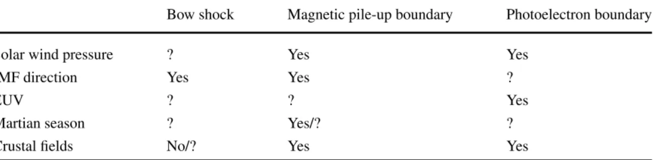
Modeling case studies suggest that the PDL can extend to cusp latitudes and 6 hours in local time away from noon (Wang et al.2003). Predicted density depletion factors (for sim-ilar solar wind conditions) range from 1.2 (Lyon 1994) to 10 (Siscoe et al.2002). Table 1
summarizes reported depletion layer dependencies on solar wind conditions. In some mod-els, depletion factors and layer thicknesses diminish with increases in the IMF clock angle away from northward in the plane perpendicular to the Sun-Earth line (Siscoe et al. 2002), while in others they increase (Table 5 of Wang et al. 2004a; Pudovkin et al. 1995, 2001,
2002). Wang et al. (2004a) presented results from a parametric study indicating that deple-tion layer widths decrease with increasing solar wind magnetosonic Mach number, increase with increasingly northward IMF Bz strength, increase as the (clock angle) component of the IMF in the plane perpendicular to the Sun-Earth line rotates away from due northward, and remain almost constant as the dipole tilt increases. Wang et al. (2004a) also concluded that density depletion factors increase and then decrease as the solar wind magnetosonic Mach number increases, increase but then decrease as with increasingly northward IMF Bz
strength, increase slightly as the IMF clock angle increases, and decrease as the dipole tilt increases. Simulation results presented by Maynard et al. (2004) indicate that depletion lay-ers form just outside the dayside magnetopause even for southward IMF orientations when the IMF has a finite component along the Sun-Earth line and/or there is a strong dipole tilt, because reconnection moves to higher latitudes. Furthermore, they indicate depletion layers forming poleward of the cusps during intervals of very strongly southward IMF orientations. Case and statistical studies of single-point in situ spacecraft observations provide support for some of these predictions. On the subsolar magnetopause, both layer thicknesses and depletion factors diminish when the IMF turns southward (Phan et al. 1994; Slivka et al.
2015) or radial (Anderson and Fuselier1993). Farrugia et al. (1995) reported that the layer becomes more pronounced for low solar wind Mach numbers, while Anderson et al. (1997) reported a pronounced layer for high solar wind Mach numbers when the magnetosphere is compressed by high solar wind dynamic pressures, solar wind densities are large, and Alfvén velocities are low. Maynard et al. (2004) reported that the layer shifts to the region behind the quasi-perpendicular bow shock. Finally, a pronounced depletion layer has indeed been observed on the high latitude magnetopause during an interval of southward IMF orientation (Moretto et al. 2005). Contrary to model predictions, the depletion layer may become less prominent for small IMF cone angles (Anderson and Fuselier 1993). Soft X-ray images, like those proposed in this work, could be used to discriminate between these predictions and examine others yet to be tested.
Song et al. (1990) and Song and Russell (1992) reported observations of anticorrelated density enhancements and magnetic field strength depressions just upstream from the subso-lar magnetopause and interpreted these observations in terms of standing slow mode waves. Southwood and Kivelson (1992, 1995) illustrated how a slow mode wave standing in the magnetosheath could result in a region with enhanced densities and depressed magnetic field strengths. Magnetic field lines within this region would have greater components par-allel to the Sun-Earth line than those either further upstream in the magnetosheath proper
Table 1 Depletion layer predictions and observations
Property Predicted dependence Control parameter Ref. Observation Thickness Decreases with Increasing
magnetosonic Mach number
1, 2, 9
Increases with Increasing positive IMF Bz
3 Present at subsolar magnetopause for IMF Bz>0, absent for IMF
Bz<0 (Phan et al.1994)
Present for large negative IMF Bz
on polar magnetopause (Moretto et al.2005)
Increases slightly with
Increasing IMF clock angle
3 Shows little effect
along Sun-Earth line with
Increasing IMF cone angle
3
Is greater for 15◦than 0◦or 30◦
dipole tilt 3
Increases for Increasing
Sun-Earth-Observer Angle
4
Density
depletion First decreases thenincreases as Magnetosonic Machnumber increases from 5.3 to 8.8
3 Larger for low Alfvénic Mach number (Farrugia et al.1995) Larger for high Alfvénic Mach number (Anderson et al.1997) First increases then
decreases as IMF B21 nTzincreases 2 to 3 Much greater for Bz
>0 than Bz<0 (Phan et al.1994; Anderson
et al.1997) Increases
non-monotonically as IMF clock angleincreases 3 Magnetic barrier (densitydepletion) increases with increasing clock angle (Pudovkin et al.1995,2001,2002)
Decreases as IMF clock angle
increases 5
Shows little effect along Sun-Earth line with
Increasing IMF cone
angle 3 Becomes more prominent withincreasing cone angle (Anderson and Fuselier1993) Shifts to region behind quasi-perpendicular shock (Maynard et al.2004)
Decreases with Increasing dipole tilt 3 Increases with Increasing dipole tilt
(or Bx)
6 Decreases with Increasing
Sun-Earth-Observer angle 4 Enhanced densities in standing slow mode waves
Absent for all IMF orientations 3, 7 Slow mode waves exist (Song et al.
1990; Song and Russell1992) Present for non-zero IMF cone angles 8 Should be interpreted as
transmitted IMF discontinuities (Hubert and Samsonov2004) References: 1—Zwan and Wolf (1976); 2—Miura (1984); 3—Wang et al. (2004a); 4—Wang et al. (2003); 5—Siscoe et al. (2002); 6—Maynard et al. (2004); 7—Samsonov and Hubert (2004); 8—Lee et al. (1991); 9—Farrugia et al. (2000)
or downstream in the depletion layer. Lee et al. (1991) identified the anticorrelated features in two-dimensional incompressible MHD simulations whenever there was a magnetic field component parallel to the Sun-Earth line. However, Wang et al. (2004b,c) and Samsonov and Hubert (2004) were unable to find any such features in global MHD simulations for any IMF orientation. Hubert and Samsonov (2004) concluded that the anticorrelated density enhancements and magnetic field strength decreases were simply antisunward propagating solar wind features caught just before they encountered the magnetopause, which prompted a comment (Song et al. 2005) and reply (Hubert and Samsonov 2005). The issue remains unsettled, but could be addressed by imaging the structure of the inner magnetosheath.
Dawn/dusk asymmetries in magnetosheath densities may control the occurrence of re-connection and the entry of solar wind/magnetosheath plasma into the magnetosphere. This entry results in the formation of low-latitude boundary layers with magnetosheath-like plasma at densities lower than those in the magnetosheath. Observations indicating greater densities in the dawnside than duskside low-latitude boundary layer (LLBL, Hasegawa et al.
2003) and magnetotail plasma sheet (Wing et al.2005) suggest greater pre- than post-noon magnetosheath densities and/or plasma entry. Walters (1964) argued that the presence of a Parker spiral IMF embedded in the flowing solar wind plasma would indeed result in greater dawnside than duskside magnetosheath densities, particularly during intervals of low solar wind Mach number. Global MHD models confirm this prediction for spiral IMF orientations, with asymmetries that increase for decreasing solar wind Mach number (Walsh et al.2012b). Observationally, Paularena et al. (2001), Nˇemeˇcek et al. (2002), and Longmore et al. (2005) report greater densities in the dawnside magnetosheath than in the duskside magnetosheath. However, each of these studies concluded that the density asymmetry was unrelated to the IMF orientation. By contrast, Walsh et al. (2012b) reported asymmetries in the expected sense. A statistical survey reported by Dimmock and Nykyri (2013) found no evidence for any dawn/dusk density asymmetry, but Dimmock et al. (2016) went on to show that the expected asymmetries were in fact present, but only in the region immediately outside the magnetopause. Finally, note that greater densities and consequently enhanced plasma betas should inhibit reconnection. Rather than resulting from asymmetric magnetosheath densi-ties, observations of enhanced densities in the dawnside boundary layer and plasma sheet may indicate the preferential operation of one or more diffusive entry processes.
2.1.5 Earth’s Bow Shock
Simulations for the solar wind’s interaction with the Earth’s magnetosphere require accu-rate values for the polytropic index γ which represents the ratio of specific heats (Cp/Cv)
and closes the set of magnetohydrodynamic equations. Determining the polytropic index is important because it controls phenomena as diverse as the degree of heating in magnetic re-connection (Hesse and Birn1992) and magnetosheath flow deflections (Nishino et al.2008). Theoretical values for γ range from 2 (for an adiabatic gas with two degrees of freedom perpendicular to the magnetic field), through 5/3 (for an adiabatic gas with three degrees of freedom), 1.5, and 1.33 (when there is a heat flux escaping from the magnetosheath into the solar wind, Nishino et al. 2008), to 1 (for an isothermal gas). Observationally-inferred values for γ are almost as diverse, ranging from 1.67 (Russell et al. 1983), through 1.76 (Farris et al.1991) and 1.85 (Tatrallyay et al.1984), to 2 (Zhuang and Russell1981).
Density jumps at the bow shock provide crucial information concerning γ (Farris et al. 1991). Following Spreiter et al. (1966), the jumps are a function of both γ and the upstream solar wind magnetosonic Mach number (MMS), i.e., ρ/ρsw= (γ + 1)M2MS/
[(γ −1)M2