A Merged Search-Coil and Fluxgate Magnetometer Data Product for Parker Solar Probe FIELDS

HAL Id: hal-02475273

https://hal.archives-ouvertes.fr/hal-02475273

Submitted on 11 May 2020

HAL is a multi-disciplinary open access

archive for the deposit and dissemination of

sci-entific research documents, whether they are

pub-lished or not. The documents may come from

teaching and research institutions in France or

abroad, or from public or private research centers.

L’archive ouverte pluridisciplinaire HAL, est

destinée au dépôt et à la diffusion de documents

scientifiques de niveau recherche, publiés ou non,

émanant des établissements d’enseignement et de

recherche français ou étrangers, des laboratoires

publics ou privés.

Trevor A. Bowen, Stuart D. Bale, John W. Bonnell, Thierry Dudok de Wit,

Keith Goetz, Katherine Goodrich, Jacob Gruesbeck, Peter R. Harvey,

Guillaume Jannet, Andriy Koval, et al.

To cite this version:

Trevor A. Bowen, Stuart D. Bale, John W. Bonnell, Thierry Dudok de Wit, Keith Goetz, et al.. A

Merged Search-Coil and Fluxgate Magnetometer Data Product for Parker Solar Probe FIELDS.

Jour-nal of Geophysical Research Space Physics, American Geophysical Union/Wiley, 2020, 125, pp.7813.

�10.1029/2020JA027813�. �hal-02475273�

T. A. Bowen1 _{, S. D. Bale}1,2 _{, J. W. Bonnell}1 _{, T. Dudok de Wit}3 _{, K. Goetz}4 _{, K.}

Goodrich1 _{, J. Gruesbeck}5 _{, P. R. Harvey}1 _{, G. Jannet}3_{, A. Koval}6,7_{, R. J. MacDowall}5 _,

D. M. Malaspina8 _{, M. Pulupa}1 _{, C. Revillet}3 _{, D. Sheppard}5_{, and A. Szabo}7

1_{Space Sciences Laboratory, University of California Berkeley, Berkeley, CA, USA,}2_{Physics Department, University of}

California Berkeley, Berkeley, CA, USA,3_{LPC2E, CNRS and University of Orléans, Orleans, France,}4_{School of Physics}

and Astronomy, University of Minnesota, Twin Cities, Minneapolis, MN, USA,5_{Planetary Magnetospheres Laboratory,}

NASA Goddard Space Flight Center, Greenbelt, MD, USA,6_{Goddard Planetary Heliophysics Institute, University of}

Maryland, Baltimore County, Baltimore, MD, USA,7Heliospheric Physics Laboratory, NASA Goddard Space Flight Center, Greenbelt, MD, USA,8_{Laboratory for Atmospheric and Space Physics, University of Colorado Boulder, Boulder,}

CO, USA

Abstract

NASA's Parker Solar Probe (PSP) mission is currently investigating the local plasma environment of the inner heliosphere (<0.25 R_⊙) using both in situ and remote sensing instrumentation. Connecting signatures of microphysical particle heating and acceleration processes to macroscale heliospheric structure requires sensitive measurements of electromagnetic fields over a large range of physical scales. The FIELDS instrument, which provides PSP with in situ measurements of

electromagnetic fields of the inner heliosphere and corona, includes a set of three vector magnetometers: two fluxgate magnetometers (MAGs) and a single inductively coupled search-coil magnetometer (SCM). Together, the three FIELDS magnetometers enable measurements of the local magnetic field with a bandwidth ranging from DC to 1 MHz. This manuscript reports on the development of a merged data set combining SCM and MAG (SCaM) measurements, enabling a high fidelity data product with an optimal signal-to-noise ratio. On-ground characterization tests of complex instrumental responses and noise floors are discussed as well as application to the in-flight calibration of FIELDS data. The algorithm used on PSP/FIELDS to merge waveform observations from multiple sensors with optimal signal-to-noise characteristics is presented. In-flight analysis of calibrations and merging algorithm performance demonstrates a timing accuracy to well within the survey rate sample period of ∼340 μs.

1. Introduction

The in situ measurements of coronal heating, solar wind acceleration, and energetic particle transport made by NASA's Parker Solar Probe (PSP) will likely answer many fundamental questions relating to the helio-sphere and astrophysical plasmas (Fox et al., 2016). The FIELDS instrument on PSP provides measurements of the electric and magnetic fields (Bale et al., 2016) required to achieve the principal objectives. The mea-surements made by FIELDS are complemented by in situ meamea-surements of the solar wind and coronal plasma through the Solar Wind Electrons Alphas and Protons (SWEAP, Kasper et al., 2016) investigation; energetic particles through the Integrated Science Investigation of the Sun (IS⊙IS, McComas et al., 2016); and white light images from the Wide-Field Imager for Solar Probe (WISPR, Vourlidas et al., 2016). Accomplishing the scientific objectives of PSP requires observations of magnetic and electric fields over a wide bandwidth and large dynamic range. FIELDS measures electric field and potential fluctuations ranging from DC to 19.2 MHz with a diverse combination of survey mode waveform, burst mode waveform, and spectral observations made by the FIELDS Radio Frequency Spectrometer (RFS, Pulupa et al., 2017), Digital Fields Board (DFB, Malaspina et al., 2016), and Time Domain Sampler (TDS, Bale et al., 2016). Magnetic field instrumentation consists of a suite of three magnetometers: two vector fluxgate magnetometers (MAGs) and a single vector search-coil magnetometer (SCM) located on boom extending behind the spacecraft and within the umbra of the PSP thermal protection system (TPS).

The two fluxgate magnetometers, built at Goddard Space Flight Center (GSFC), provide vector mea-surements of DC and low-frequency (LF) magnetic fields with a maximum survey sample (Sa) rate of

Key Points:

• We develop a technique to merge search-coil and fluxgate magnetometer measurements • In-flight analysis shows that

calibrations are accurate to within 100μs

Correspondence to:

T. A. Bowen, tbowen@berkeley.edu

Citation:

Bowen, T. A., Bale, S. D., Bonnell, J. W., Dudok de Wit, T., Goetz, K., Goodrich, K., et al. (2020). A merged search-coil and fluxgate magnetometer data product for Parker Solar Probe FIELDS. Journal of Geophysical Research: Space Physics, 125, e2020JA027813. https://doi.org/ 10.1029/2020JA027813

Received 16 JAN 2020 Accepted 27 MAR 2020

Accepted article online 22 APR 2020

©2020. American Geophysical Union. All Rights Reserved.

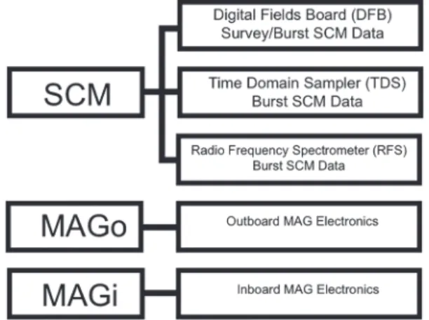
Figure 1. Block diagram of FIELDS magnetometer suite. A detailed block

diagram of the entire FIELDS instrument can be found in Bale et al. (2016).

𝑓max

sv𝑦 =292.969 Sa/s. These LF measurements are accompanied by

mea-surements from the FIELDS SCM LF windings, which are sensitive from ≈3 Hz to 20 kHz. The SCM sensor x axis additionally contains a second midfrequency (MF) winding, sensitive from ≈10 kHz to 1 MHz. Dur-ing perihelion encounters, the SCM is continuously sampled by the DFB typically at f_svy = 292.969 Sa/s, though a maximum rate of 18,750 Sa/s is theoretically possible (Malaspina et al., 2016). When possible, data are additionally acquired during the aphelion cruise phases at reduced sample rates in accordance with allowed telemetry and spacecraft oper-ations. Burst mode waveforms for the LF axis may be sampled up to a maximum rate of 150 kSa/s by the DFB; the MF channel can be sam-pled at 1.92 MSa/s by the TDS and incorporated in the spectral products generated by the RFS. Generally, the DFB, RFS, and TDS are highly configurable and generate a variety of waveform and cross and autospec-tral matrix data products at various cadences. Figure 1 shows a simple schematic of the FIELDS magnetometer sensor and sampling electronics; comprehensive discussion of the FIELDS instrument and data prod-ucts are available in the respective instrument papers (Bale et al., 2016; Malaspina et al., 2016; Pulupa et al., 2017).

Observational signatures of physical processes occurring in astrophysical plasmas, such as the solar wind and corona, are commonly sensitive to properties of the mean magnetic field: for example, electromagnetic wave-vector polarizations (He et al., 2011; Podesta & Gary, 2011); magnetic compressibility (Alexandrova et al., 2013; Bale et al., 2009); variance and wave-vector anisotropies (Chen et al., 2010; Horbury et al., 2008; 2012); MHD Elsässer and Poynting flux (Balogh et al., 1999; McManus et al., 2020); helical signatures of tur-bulence at kinetic scales (Howes & Quataert, 2010; Leamon et al., 1998; Woodham et al., 2018); and magnetic reconnection (Phan et al., 2018). Though microphysical processes in the solar wind are sensitive to the mean magnetic field , they frequently occur on fast timescales with small-amplitude magnetic signatures. Accom-plishing the scientific objectives of PSP thus inherently requires in situ observations of magnetic fields over large bandwidths and dynamic ranges. Through combining both fluxgate and search-coil measurements, FIELDS is capable of observing the in situ magnetic field of the inner heliosphere with a bandwidth from DC to 1 MHz and 115 dB of dynamic range (Bale et al., 2016).

Recently, missions with multisensor observational suites have moved toward merged data products com-posed of synchronous measurements from multiple instruments, combined to employ optimal qualities of the separate sensors. Alexandrova et al. (2004) used a discrete wavelet transform to merge CLUSTER flux-gate and search-coil data to study waves downstream of a shock (Balogh et al., 2001; Cornilleau-Wehrlin et al., 2003). Chen et al. (2010) use a similar method to study the variance anisotropy of kinetic turbu-lence in the sub-proton range with CLUSTER. Additionally, Kiyani et al. (2009) perform measurements of scaling functions of the transition from the MHD to kinetic turbulence through continuous analysis of a combination of CLUSTER fluxgate and SCM observations. These previous efforts to combine fluxgate and search-coil data, though made in-flight and without specific optimization toward instrument design and operation, have proved the utility and applicability of multirate data fusion methods in space plasma physics (Hall, 1992). More recently, programmatic efforts to perform quantitative end-to-end testing on the Magneto-spheric Multiscale Mission (MMS) search-coil and digital and analog fluxgate magnetometers have enabled the development of an optimized merged data set with automated calibration pipeline (Fischer et al., 2016; Le Contel et al., 2016; Russell et al., 2016; Torbert et al., 2016).

The FIELDS SCM and MAG share a master clock and were designed with partially overlapping bandwidths, enabling the combination of individual sensors into a single merged data set. This manuscript outlines the process used to produce survey data product using merged SCM and MAG (SCaM) measurements with a spectral composition that retains an optimal signal-to-noise ratio. Section 2 provides an overview of pre-flight ground testing and instrument characterization, as well as in-pre-flight calibration routines. Section 3 presents the algorithm used to combine the FIELDS magnetometer data into a merged product with optimal signal-to-noise characteristics. Section 4 provides a summary of our in-flight verification of the calibration and a quantitative analysis of the performance of the merged survey data and discusses merging survey rate data with DFB burst data (Malaspina et al., 2016).

(a)

(b)

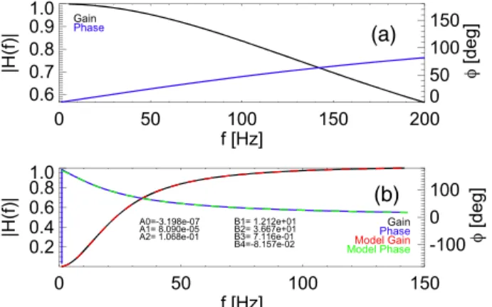
Figure 2. (a) MAGo frequency response is dominated by single pole Butterworth filter response tuned to−3 dB at the survey mode Nyquist frequency (𝑓max

sv𝑦 ∕2). (b) SCM frequency response determined from a spectral analyzer. A

four-pole, two-zero fit analytical fit is performed to the empirically determined function.

2. FIELDS Calibration

2.1. Fluxgate Magnetometers (MAGs)

The two fluxgate magnetometers, designed and fabricated at NASA/GSFC, measure DC and LF fluctuating magnetic fields. They are placed 1.9 and 2.7 m from the spacecraft and are respectively referred to as the inboard (MAGi) and outboard (MAGo) sensors. The heritage of the PSP/FIELDS MAGs dates to the 1960s NASA Explorer 33 mission (Acuna, 1974, 2002; Ness et al., 1971). Many iterations of the instrument cur-rently operate on both NASA heliophysics and planetary science missions (Acuña, 2002; Acuña et al.,2008; Connerney et al., 2015, 2017; Kletzing et al., 2013; Lepping et al., 1995). The PSP fluxgate magnetometers have a maximum survey mode sample rate of𝑓max

sv𝑦 = 292.969 Sa/s. The MAG data are typically

down-sampled by factors of two with antialiasing performed with a Bartlett filter. Generally, MAGi is run at a lower sample rate in order to meet telemetry constraints imposed by the spacecraft. The lower cadence measurements still allow for diagnosis of magnetic noise associated with spacecraft-generated magnetic fields. The primary science instrument for the DC magnetic fields is MAGo, which is less sensitive to spacecraft-generated fields due to its positioning on the spacecraft boom.

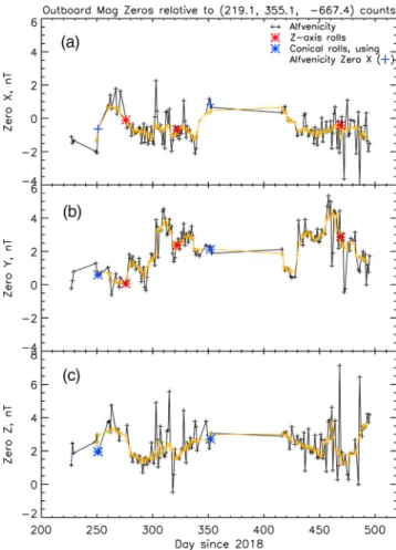
The complex transfer functions associated with the MAGs, shown in Figure 2a, are dominated by a single pole low-pass Butterworth filter used for antialiasing purposes tuned to −3 dB at the max sample rate Nyquist frequency (𝑓_sv𝑦N𝑦≈146.5 Hz) (Acuña et al., 2008; Connerney et al., 2015, 2017). Due to the low-pass charac-teristics of the Butterworth transfer function, the MAGs are sensitive to the DC magnetic fields associated with the spacecraft (Belcher, 1973; Ness, 1970; Ness et al., 1971). Typically, the minimization of such fields is performed through magnetic control programs (Ness, 1970; Musmann, 1988). For PSP, a strict magnetic cleanliness program was followed during design and development. Once in space, driven spacecraft maneu-vers are used to establish the magnetometer zero offsets relative to the ambient field, for example (Acuña, 2002; Connerney et al., 2015). However, similar results can be accomplished without controlled maneuvers through statistical analysis of noncompressive Alfvénic rotations in the solar wind (Belcher, 1973; Leinweber et al., 2008). Several multisensor techniques to determine sensor zeros have been developed using gradio-metric principles, for example (Ness et al., 1971), and comparison with scalar magnitude instruments, for example (Olsen et al., 2003; Primdahl et al., 2006). Additionally, solar wind electron beams, sensitive to the mean field direction, can be used in calibrating fluxgate offsets (Connerney et al., 2015; Plaschke et al., 2014). For PSP, the attitude and pointing requirements of the spacecraft preclude the use of controlled maneu-vers during perihelion, spacecraft rolls (both sun-pointed and conical rotations) are thus performed before and after each perihelion encounter to establish zero levels of the spacecraft magnetic field. In between such controlled rotations, measurements of Alfvénic rotations of the solar wind magnetic field have been implemented to track variations in the spacecraft field, allowing for an estimate of zero levels during each perihelion encounter, when controlled maneuvers cannot be performed (Leinweber et al., 2008). Figure 3 shows the offsets for MAGo over the first encounter computed using both spacecraft rolls and higher rate estimations from Alfvénic rotations. Spacecraft housekeeping and engineering data are currently under analysis in order to model the effects of variations in the solar panel array, which change orientation over

Figure 3. Magnetic field zero offsets for FIELDS/MAGo x, y, and z axes

(panels a, b, and c) over the first two encounters of PSP (respectively offset by 219.1, 355.1, and−667.4 sensor counts for demonstrative purposes). Data points (+) correspond to estimates from Alfvénic rotations of the solar wind; a seven-point median filter was used in processing the FIELDS data (orange). Offsets determined from spacecraft rotations are shown in red (sun-pointed rolls around the spacecraft z axis) and blue (conical rolls performed off sensor z axis). The blue + corresponds to the MAGo x offset determined from Alfvenic at the time of the conical roles.

the course of the orbit, on the measured DC offsets. Gradiometric tech-niques are in development to further verify and monitor offset drifts during each perihelion encounter. In addition to the removal of space-craft offsets, the vector axes of each MAG are orthogonalized using an alignment matrix determined during preflight testing. The alignment matrix is determined through the process documented in Acuña (1981) and Connerney et al. (2017) and verified by methods outlined in Risbo et al. (2003).

In addition to the removal of spacecraft offsets and sensor orthogonaliza-tion, the merged data set corrects gain and phase shifts associated with the analog Butterworth filter using a convolution of the MAG output with the linear time-invariant (LTI) inverse filter response. When appropri-ate, the digital Bartlett filter used to downsample MAG measurements is additionally inverted. Though the phase shifts associated with these low-pass filters are quite small (e.g., Figure 2) over the range of frequen-cies observed by both the MAG and SCM, the misalignment of relative phase between the MAG and SCM leads to undesirable artifacts in the merged data product. Correction for complex instrumental response (i.e., filter gain and phase) is not implemented in the unmerged MAG data.

2.2. SCM

The PSP/FIELDS SCM was designed at Laboratoire de Physique et Chimie de l'Environnement et de l'Espace (LPC2E) in Orléans, France, and is nearly identical to the search coils that have been manufactured and delivered for the Solar Orbiter and TARANIS missions (Maksimovic, 2020; Séran & Fergeau, 2005). The SCM, mounted on the end of the spacecraft magnetometer boom 3.5 m from the spacecraft bus that con-sists of three mutually orthogonal inductive coils, is tailored to study the magnetic fields of the inner heliosphere (Bale et al., 2016) at frequencies ranging from≲10 Hz to 20 kHz. The SCM sensor x-axis has an additional coil with bandwidth of 10 kHz to 1 MHz. A flat frequency response is attained in each coil using secondary windings to generate flux feedback at the resonance frequency of the primary sensor coil (Séran & Fergeau, 2005). The survey mode waveform data, typically captured at a rate of

𝑓max

sv𝑦 = 292.969 Sa/s, are sampled and processed by the FIELDS DFB

(Malaspina et al., 2016). In addition to continuous survey mode waveform data, the DFB provides a highly configurable set of operational modes, which can be modified in-flight to generate a diverse set of burst waveform and spectral data products. The secondary flux feedback winding allows the DFB to inject a programmable calibration signal into the SCM. The response of the SCM to the injected stimulus is captured by the DFB and TDS, and the instrumental transfer function can accordingly be determined in-flight.

Figure 2b shows the gain and phase characteristics of the FIELDS SCM x-axis, which were determined empirically onground using a spectral analyzer. A complex rational function with four poles and two zeros:

R(i𝜔) = A0+i𝜔A1

(B₀−B₂𝜔2_{) +i}𝜔(B

1−B3𝜔2)

(1) is fit to the response using the least square estimation techniques developed by Levy (1959).

The strong gain and phase shifts in the SCM instrumental response function must be compensated to obtain an estimate of the observed magnetic field in physical units. During prelaunch integration and testing dif-ferent methods to invert the SCM frequency response were explored: convolution kernel methods and a windowed fast Fourier transform (FFT) algorithm similar to techniques used in Le Contel et al. (2008) and Robert et al. (2014). Preflight Monte Carlo simulations testing on synthetic data suggested that convolu-tion in the time domain generated fewer spectral artifacts in the calibrated time series than a windowed FFT algorithm. Compensation filters are developed using the inverse FFT of the response function on an

abscissae of 2,048 frequencies, corresponding to a 2,048 tap (all zero) LTI finite impulse response (FIR) filter (Oppenheim & Schafer, 1975). The filters are noncausal, such that real-time merging of data (e.g., on the spacecraft) is not possible; the future development of causal FIR filters for onboard merging presents an opportunity to increase scientific returns from telemetry limited missions.

3. Merging

Many algorithms for merging data from multiple sensors, occasionally referred to as data fusion, were ini-tially developed in the context of radio system engineering as a method to optimize signal-to-noise ratios and correct for signal loss due to stochastic fluctuations impacting transmission (Brennan, 1959; Kahn, 1954). Recent research has demonstrated the applicability of data fusion in merging magnetic field measurements from multiple sensors onboard a single spacecraft (Alexandrova et al., 2004; Chen et al., 2010; Kiyani et al., 2009). However, MMS is the first mission where significant effort was made to design sensors with synchro-nized timing with prelaunch end-to-end characterization of sensor performance intended to enable optimal merging of in-flight magnetic field data (Fischer et al., 2016; Torbert et al., 2016). The shared clock between the PSP/FIELDS SCM and MAGs, in addition with their simultaneous continuous survey mode operation, facilitates a merged SCM and MAG (SCaM) data product. In order to produce the merged SCaM data prod-uct, accurate representations for the complex frequency responses for the individual sensors are required. In addition to the individual characterization of the instruments, multiple efforts were made to intercalibrate the sensors; however, no strict end-to-end calibration was performed as in Fischer et al. (2016). Original ground testing was performed at the Acuña Test facility using FIELDS engineering model hardware; sub-sequent testing was performed on flight model hardware during final stages of integration onto the PSP spacecraft, verifying the instrument gain and phase characteristics. The merged SCaM data ideally attains optimal signal-to-noise characteristics, such that an accurate characterization of the individual MAG and SCM sensor noise floors is necessary, in addition to an accurate description of the instrumental transfer functions.

Optimal signal-to-noise merging coefficients are constructed assuming that the noise floors of each reach instrument represent incoherent, mean-zero, Gaussian processes. The spectral composition of the instru-mental noise was determined during ground testing. The SCM sensitivity was characterized at the magnetic test facility in Chambon-la-Forêt. In addition to the internal sensor noise, the DFB analog electronics as well as analog to digital conversion (quantization) of the SCM signal contribute to the end-to-end instrumental noise. The end-to-end noise floor of the MAGs, incorporating quantization and analog electronic noise, was determined in laboratory using measurements taken over several hours inside of a μ-metal container. The FIELDS SCaM merging procedure is designed to maintain an optimized signal-to-noise ratio. The SCaM merging algorithm assumes that the environmental field, Bext, is separately observed in each sensor as a coherent signal in superposition with incoherent, mean-zero, uncorrelated noise: nSCMand nMAG.

BMAG=Bext(t) + nMAG(t), (2)

BSCM=Bext(t) + nSCM(t). (3)

The merged signal, B_m, is given as a linear combination of the individual sensors, weighted by coefficients

𝛼MAGand𝛼SCM, which maintain an optimal signal-to-noise ratio.

As instrumental noise from each sensor has different spectral characteristics, we develop frequency-dependent merging coefficients through consideration of the spectral representation of the linear combina-tion of signal and noise terms

̃B_m(𝜔) = 𝛼_MAG̃B_MAG(𝜔) + 𝛼_SCM̃B_SCM(𝜔), (4) Ñm(𝜔) = √ 𝛼2 MAGñ 2 MAG+𝛼 2 SCMñ 2 SCM, (5)

where the merged noise Ñm(𝜔) corresponds to the error of each signal, weighted and added in quadrature

(Brennan, 1959; Kahn, 1954). The condition𝛼1+𝛼2=1is required such that the merged signal is equal to the coherent environmental field observed by each sensor.

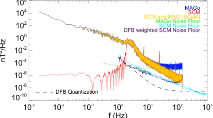
Figure 4. Empirically determined noise floors of PSP FIELDS MAGo x, y,

and z axes (blue, green, and black) and the SCM low-frequency x, y, and z axes with the DFB sampling in a high-gain state (red, orange, and purple) rotated into MAGo sensor coordinates. The DFB quantization

corresponding the high-gain SCM state is additionally shown (dashed line).

Because signal amplitudes are ideally equal in either sensor, optimiz-ing the ratio Bm∕Nmleads to frequency-dependent solutions for𝛼1(𝜔) and𝛼2(𝜔), which are independent of the environmental signal, and determined by the spectral composition of the noise floors:

𝛼MAG(𝜔) = ñ2 SCM ñ2 MAG+ñ 2 SCM , (6) 𝛼SCM(𝜔) = ñ2 MAG ñ2 MAG+ñ 2 SCM , (7) where ñ2 MAGand ñ 2

SCMare computed as the spectral densities of the

instru-ment noise. For FIELDS, the coefficients𝛼MAGand𝛼SCMcorrespond to an

effective weighting in instrumental gain, which preserves an optimized signal-to-noise ratio for the merged SCaM data product. The SCM sen-sor coordinate system is not initially aligned with the MAG sensen-sor axes, accordingly a rotation matrix R is applied to bring the SCM measurements in sensor coordinates, B′

SCM, into alignment with the MAG coordinate

system, R = ⎛ ⎜ ⎜ ⎝ 0.8165 −0.4082 −0.4082 0.0000 −0.7071 0.7071 −0.577 −0.577 −0.577 ⎞ ⎟ ⎟ ⎠, (8) BSCM=R · B′SCM. (9)

Adhering to an optimal signal-to-noise merger, spectral composition of the noise of the rotated SCM vector time series in MAG sensor coordinates is then taken as the quadrature weighted error of the SCM sensor axis noise, assuming independence in each sensor channel: that is,

ñ2

SCMx(𝜔) = R

2

xx′ñ2_SCMx′+R2_x𝑦′ñ_SCM𝑦2 ′+R2_xz′ñ2_SCMz′. (10)

The MAG orthogonalization matrix and rotation from sensor to spacecraft coordinates is approximately equal to the identity matrix such that the measured noise floor for each sensor axis is used without contribution from the other axes.

Figure 4 shows empirically determined noise floors for both the SCM and MAGo associated with mean-zero stochastic fluctuations limiting each sensors sensitivity. Merging coefficients are obtained using

Figure 5. Nonlinear least square fit of three-pole, one-zero rational

function to_𝛼MAGfor f_>f₀with f₀=2Hz. At 2 Hz,_𝛼MAGis set to unity, the fit function is constrained to maintain a continuous value and first derivative, such that an extremum is obtained.

equation (6). Since the empirically determined noise spectrum is continu-ous, a smooth weighting of the merged signals is obtained by approximat-ing the MAG mergapproximat-ing coefficient usapproximat-ing a real-valued rational function of the form ̂𝛼MAG(𝑓) = N(𝑓) D(𝑓)= ∑n 0An𝑓n 1 +∑m₁ Bm𝑓m . (11)

Below f0 = 2Hz, the sensitivity of the SCM drops significantly and the full MAG signal is used, that is,𝛼MAG = 1for f ≤ 2 Hz. Above 2 Hz,

equation (11) is applied. The coefficients and order of the fit rational func-tion are determined using nonlinear least squares fitting (Markwardt, 2009). Constraints are imposed on ̂𝛼MAG(𝑓) to ensure continuity such

̂𝛼MAG(𝑓0) = 1and ̂𝛼MAG′ (𝑓0) = 0, where f0 = 2Hz. Figure 5 shows the n =1and m = 3 (one-zero and three-pole) fit for̂𝛼MAG.

Fitting𝛼MAG(f)with boundary conditions at f0=2Hz decreases available degrees of two freedom such that rational functions with three or more

(a)

(b)

Figure 6. (a) Analytical approximations of MAG and SCM merging

coefficients (y axis shown). (b) Noise floors of MAG (blue) and SCM (red); the coefficient weighted noise floors are shown for MAG (purple) and SCM (orange). The optimal noise floor is plotted in green.

fit parameters are required for a reasonable approximation. Figure 5 shows the best fit rational function (equation (11)) with three poles and one zero (e.g., m = 3 and n = 1), to the MAG merging coefficient,𝛼MAG,

with applied boundary conditions at 2 Hz. Ensuring a piecewise continu-ous merging coefficient requires constraining the function at 2 Hz to unity gain and a local extremum. For f< 2 Hz, the coefficient 𝛼MAGis

explic-itly set to unity, for example, Figure 6, while for f> 2 Hz, 𝛼MAG= ̂𝛼MAG.

The SCM coefficients are determined from𝛼_SCM=1 −𝛼_MAG. The optimal merging coefficients𝛼_MAGand𝛼_SCMare shown in Figure 6a. The weighted instrumental noise floors and the optimal merged SCaM noise floors are shown in Figure 6b.

4. Calibration and Merger of In-Flight Survey Data

During the PSP perihelion encounters, survey mode data are acquired at different cadences, typically varying with solar distance, in order to balance science objectives with telemetry constraints. When possible, the FIELDS team intends to operate the instruments with a single high data rate (292.969 Sa/s) over the entire perihelion encounter period. To date, the lowest cadence survey rate during the perihelion encounter is 73.24 Sa/s.

The calibration kernel, corresponding to the inverse response of the MAG instrument response, is weighted by the appropriate merging gain coefficients,𝛼MAG, to construct the contribution from MAGo to the merged

time series. This weighted time series subsequently undergoes calibration processes associated with orthog-onalization and spacecraft field removal used in generation of public unmerged data. The SCM is similarly calibrated using the instrumental response function with gain weighted by the merge coefficients𝛼SCM; the

gain and gain phase shifts associated with digitization by the FIELDS DFB are additionally corrected for Malaspina et al. (2016). Once convolved with calibration kernels, the SCM is rotated into the MAGo coordi-nate system. The weighted MAG time series is then interpolated onto the SCM time abscissae. Interpolation onto the SCM time tags is used to preserve the high-frequency component of the SCM without introducing artifacts associated with interpolation. The time series are directly summed to generate the merged data set with optimal signal-to-noise ratio. The merged SCaM data are considered a Level 3 (L3) data product. Power spectra from an approximate hour-long interval (220 _{samples at 292.969 Sa/s) starting 5} Novem-ber 2018/00:00 during the first PSP perihelion is highlighted in Figure 7 to demonstrate the results of our calibration and merging algorithm. Power spectra for each of the MAG, SCM, and SCaM time series are computed as an ensemble average of eight power spectra of 217 _{samples. We note excellent qualitative}

Figure 7. Power spectral densities of observed magnetic field in the

spacecraft coordinate y direction from≈1-hr interval (5 November 2018/00:00–01:00) calculated with MAG (blue), SCM (red), and merged SCM and MAG (SCaM, orange) time series. Sensor noise floors are shown for the MAG (teal) and SCM (green). The SCM noise floor after correcting the DFB antialiasing filter gain is shown in purple. The DFB quantization level is additionally shown.

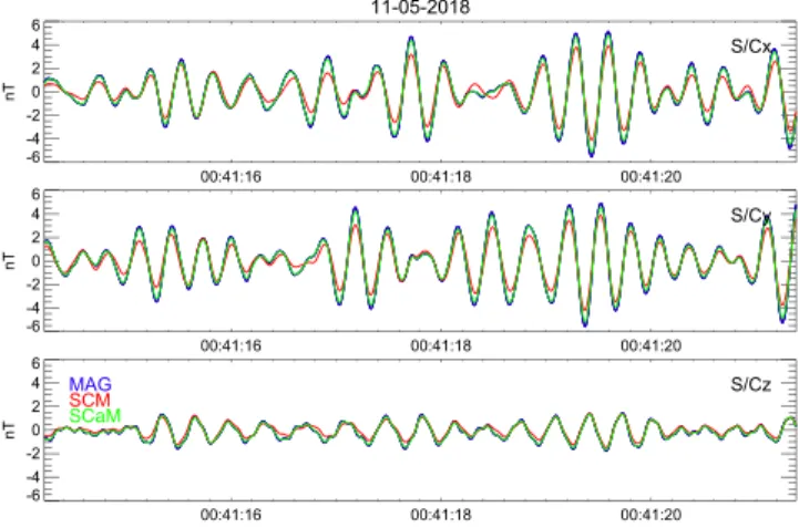
agreement between the MAG and SCaM data at low frequencies, and the SCM and SCaM data at high frequencies, in Figure 7 leads to an apparent overlapping of spectra. Figure 7 additionally shows noise floors associated with the MAG and SCM instruments. Good agreement is observed between the merged data and spectra from either individual instrument. The in-flight observed noise floor of the MAGo is consistent with on-ground measurements. The SCM noise floor performs similarly to preflight measurements; a slight increase in the sensitivity is observed relative to ground testing, which is attributable to a decrease in thermal noise in the instrument. Broadband spectral features near the crossover frequency, corresponding to coherent wave features at several hertz, are captured by both the MAG and SCM and are thus useful in analyzing the performance of the SCaM merging algorithm (Bale et al., 2019; Bowen et al., 2020). Digital filters are applied to bandpass the MAG, SCM, and merged SCaM time series to between 2 and 12 Hz in order to directly compare the time series in the crossover bandwidth, without contribution from low- or high-frequency signals. Figure 8 shows excellent qualitative agreement in phase between the three different waveforms.

Figure 8. Eight-second bandpass-filtered waveform near the merging

crossover frequency (2–12 Hz) from PSP/FIELDS survey magnetic field data in S/C coordinates. Good phase and gain agreement is observed in between the MAG (blue) SCM (red) and merged SCaM (green) time series.

However, in order to ensure quality of the merged SCaM data prod-uct, the calibrated, but unmerged, MAG and SCM observations must be analyzed to verify the conditions necessary for the weighted-gain merging algorithm developed in section 3: that is, the MAG and SCM cross-calibration, including time synchronization and gain matching, must be verified. Careful inspection of Figure 8 shows a small-gain dis-crepancy between the MAG and SCM amplitudes. Analysis of the gain discrepancy is required to ensure an artifact-free merged data product. Quantitative determination of the relative MAG and SCM gain calibra-tions is performed by separating the full day of encounter data from 5 November 2019 into 22 nonoverlapping intervals of 220_{samples (a 1-hr} interval where the SCM was in a low-gain state was omitted). The vector spectral density for each interval is estimated for both MAG and SCM sen-sors by ensemble averaging the power spectrum of 1,024 nonoverlapping subintervals computed via FFT, for example:

S_MAG(𝑓)=⟨{B_MAG(t)}†_{B

MAG(t)}⟩,

where{ … } is the Fourier transform and ⟨ … ⟩ denotes ensemble aver-aging; a Blackman-Harris window is used to prevent spectral leakage. The frequency-dependent gain is then obtained as

G(𝑓) = 10Log₁₀SSCM SMAG

.

Figure 9 shows the measured distribution of G(f) for each vector component as well as the mean at each fre-quency and the median gain error computed between 3 and 10 Hz. Systematic gain differences are measured in the x, y, and z directions of −2.67, −2.50, and −2.58 dB. Gain correction is required in order to remove artifacts associated with merging signals with unequal amplitudes. Due to the relatively stable gain discrep-ancy in frequency and time, the SCM may be gain matched to the MAG through multiplication of scaling factors (1.36, 1.33, and 1.34) for the respective x, y, and z axes. These values indicate that the typical SCM amplitude is approximately 75% of the measured MAG signal. The decrease in relative gain in the z-axis at ∼7 Hz coincides with the frequency of one of the spacecraft reaction wheels at the time of the measure-ment and does not represent a change in the relative instrumeasure-mental gain. The z-axis gain factor additionally shows some anomalous variation at frequencies less than 4 Hz; however, the merged data are predominantly composed of the MAG at these frequencies, and the effect of using a frequency-independent gain factor

Figure 9. Gain difference between SCM and MAG measured over their

shared observations range (x, y, and z axes shown in black, blue, and red). The measured distribution of gain differences is plotted as a set of points. The mean at each frequency is plotted as a solid line, while the median gain difference in each axis from 3–10 Hz is plotted as a dashed line. The average gain difference is roughly constant over this range. The feature at 7 Hz corresponds to a reaction wheel (which has a lower signal in the SCM due to the relative positioning of the sensors).

correction is minimal. These differences between on-ground and in-flight gain measurements are likely due to differences in the SCM operat-ing temperature, small perturbations to either the SCM or MAG rota-tion matrices, or small discrepancies caused by the matching between SCM and DFB, which unfortunately were not quantified due to lack of end-to-end calibration. Continued efforts to quantify and monitor vari-ations in the gain-matching coefficients will be performed throughout the mission. Additionally, both gain-matched and nominal calibrations will be available for public use; though the authors stress that use of non-gain-matched data may lead to artifacts in the transition between the MAG and SCM sensor ranges.

A quantitative determination of the accuracy of the timing between the MAG and SCM data is performed by computing the short-time Fourier transform cross-spectra of each of the three combinations of signals. The short-time cross-spectra is defined as

S12=⟨{B1(t)}†{B2(t)}⟩. (12) The argument of the cross-spectra gives the phase delay between the two signals at a given frequency arg(S12) = tan−1

(_Im{S

12)} Re{S12}

)

. As each sensor observes the same time series, zero-phase difference should exist at each

(a)

(b)

(c)

Figure 10. Distribution of measured phase delays between the MAG and SCM in spacecraft coordinates (x, y, and z) as

a function of frequency shown respectively in panels (a), (b), and (c). The solid black line shows the mean phase error at each frequency. The dashed black lines show linear phase error associated with one and two sample periods (Δt∼340μs).

frequency between the sensors. Each of the 22 intervals on 5 November 2018 used in gain calibration is sep-arated into 1,024 subintervals. The subdivision allows for the calculation of 22,528 individual cross-spectra. The distribution of phase delay as a function of frequency is then calculated between the MAG and SCM using the ensemble of cross-spectra.

Figure 10 shows the measured distributions of phase difference between the MAG and SCM obtained via cross-spectra. The MAG and SCM are shown to be in good agreement in the crossover frequencies: At 4 Hz, the mean time delay between the MAG and SCM measurements is 190, 84, and 100 μs for the respective x,

y, and z axes; the standard deviations are 76, 59, and 89 μs, respectively. For each vector component, approx-imately two standard deviations of the measured ensemble fall within 1Δt (∼340 μs). These results show that the phase alignment of the MAG and SCM is accurate to within a small-phase error in the frequencies surrounding the crossover point.

Analysis of the relative phase between the SCM and MAG observations verifies timing accuracy to within a single sample period. Additionally, quantification of the relative gain between the instruments allows for the empirical matching of the SCM signal to MAG levels such that a smooth transition over the sensor crossover range is obtained. Establishing L3 calibrations for the MAG and SCM provides time-synchronized and gain-matched signals such that the direct sum of the signals, with gains weighted by𝛼_MAGand𝛼_SCM, results in an optimal signal-to-noise-merged SCaM data product.

4.1. Merging DFB Burst Data

In addition to survey waveform data, the FIELDS DFB produces high-resolution burst data from SCM mea-surements at a maximum sample rate of fbrst=150kSa/s. For the three LF SCM windings, this is significantly higher than the instrumental 3-dB roll-off at ∼17 kHz. The DFB burst buffer, while highly configurable, typ-ically is taken as a Nbrst=219sample waveform lasting ∼3.5 s. Data from the SCaM product are combined with the DFB burst measurements to provide the LF spectral composition to contextualize the DFB bursts. The SCM transfer function is applied to the burst data using an FIR calibration kernel of Mbrst= 16,384 filter coefficients (taps); a cutoff is applied at the high-frequency SCM 3-dB roll-off (∼17 kHz) to prevent amplifica-tion of high-frequency noise. Frequencies f< fbrst∕Mbrst(e.g., ∼10 Hz for Mbrst= 16,384 and fbrst=150kSa/s) cannot be captured using a convolution kernel; however, the merged SCaM data are optimized to provide high signal-to-noise measurements in this frequency range.

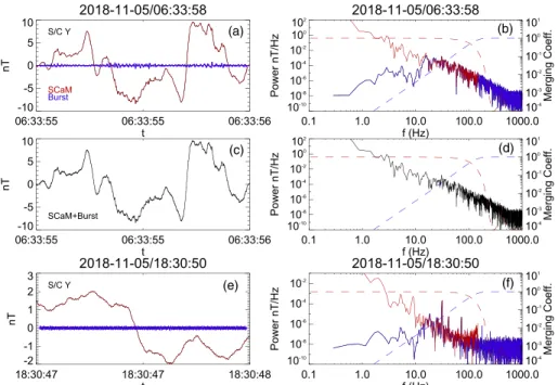
Figure 11a demonstrates a comparison of the SCaM and DFB burst waveforms from a burst on 5 November 2018/06:33:58. Figure 11b shows power spectral densities for the interval. To combine LF spectral compo-nents with the calibrated burst data, the SCaM data are interpolated onto the DFB burst time tags, which are rotated into the S/C coordinate system. At frequencies above ∼10 Hz, the SCaM data are predominantly

(a)

(c)

(b)

(d)

(e) (f)

Figure 11. (a) Burst waveform from FIELDS DFB on 5 November 2018/06:33:58 (blue) with simultaneous SCaM

(red) waveform data. (b) Power spectral density from burst interval on 5 November 2018/06:33:58 dashed lines show the corresponding merging coefficients for the DFB burst (blue) and SCaM (red). (c) Merged DFB and SCaM waveform. (d) Merged power spectral density. (e) Waveform data from DFB burst on 5 November 2018/06:33:58 with SCaM data. (f) Power spectral density from 5 November 2018/06:33:58 interval, spectral flattening in the survey waveform can occur either when the DFB quantization limit is reached or when narrowband spectral features are present above survey Nyquist frequency.

derived from the SCM, and the intrinsic noise of the DFB burst and SCaM data is thus identical; how-ever, correcting the attenuation from the DFB antialiasing filters during the SCaM calibration results in the amplification of noise in the high-frequency end of the survey waveform data. The difference in noise level between the burst and SCaM data corresponds precisely to the DFB antialiasing filter, which is taken as the weighting coefficients, shown Figures 11b, 11d, and 11e to merge the SCaM and burst data. Figure 11c shows the merged SCaM data with DFB burst waveform data; the corresponding merged power spectral density is depicted in Figure 11d.

A second burst interval from 5 November 2018/18:30:50 is shown in Figures 11e and 11f. On occasion, spec-tral flattening is observed in the high end of the SCM and SCaM survey bandwidth, for example, Figure 11f. This effect is associated with correcting the DFB antialiasing filter in portions of the bandwidth where the environmental signal is under the instrumental noise floor. Additionally, ongoing efforts are underway to characterize narrowband spectral noise from the spacecraft and its effect on magnetic field measurements (Bowen et al., 2020).

4.2. In-Flight Issues With SCMx Axis

Since March 2019, the LF B_x channel of the SCM has deviated from nominal operation whenever the sensor is shaded by the TPS, for example, during perihelion encounters. The main symptoms of this anomaly are a much higher sensitivity to periodic current surges in the SCM heater and a drop in sen-sitivity in the LF waveform channels. This drop is equivalent to the response of an additional first-order high-pass filter with a cutoff at 1 kHz. This sudden change in sensitivity mostly impacts measurements of Bx below approximately 600 Hz. The three components of the SCM are rotated in the frame of the

MAG before merging. Accordingly, the anomaly in one single channel will affect all three vector compo-nents in the S/C spacecraft coordinates, making it impossible to properly merge the signals from the two instruments. By rotating the MAG measurements into the SCM frame, it is possible to merge measure-ments in the SCM y and z axes. For PSP's first encounter, the full vector merged product in spacecraft and RTN coordinates will be produced. For later encounters, a 2-D merged product will be distributed using the SCM y and z axes. Consequently, the MAG is the only remaining three-axis measurement

operating at survey sample rates. The degraded phase and amplitude response of the SCM maintain remarkable stability, which suggests that it remains possible to deliver properly calibrated burst data at frequencies above ˜600 Hz

5. Conclusion

This manuscript reports on the development, implementation, and performance of an algorithm to merge magnetic field observations from the PSP/FIELDS fluxgate (MAG) and search coil (SCM) to create a merged SCM and MAG (SCaM) data product. The techniques used for PSP/FIELDS are similar to efforts made by Fischer et al. (2016) to combing magnetic field measurements from instrumentation on MMS, which attempt to maintain optimal signal-to-noise characteristics. These merging algorithms have heritage from techniques developed in radio systems engineering for linear diversity combining (Brennan, 1959; Kahn, 1954). The optimal merging method takes into account sensor design and operation of the MAG and SCM instrumentation, in order to construct a merged data product with spectral composition, which smoothly transitions between the MAG at low frequencies and the SCM at high frequencies with a crossover between ∼3–10 Hz. In the crossover range of frequencies, both sensors contribute significantly to the merged SCaM data product. Using in-flight analysis of the calibrated FIELDS observations, we demonstrate that the MAG and SCM sensors are in systematic agreement to within a small fraction of a sample period (<340 μs), enabling a smooth transition between dominant signal in the crossover range without phase distortion of the measured waveforms. A small deviation in gain (∼2 dB), likely due to temperature effects, between the sensors is measured, which impacts the merging procedure and requires ongoing analysis and correction. Additionally, the merging algorithm presented is used to combine burst data from the SCM, acquired by the FIELDS DFB at a 150-kSa/s sample rate, with survey rate data from the MAG and SCM at lower fre-quencies. The merged DFB burst data allow for analysis of magnetic field signals from DC to the SCM LF cutoff (17 kHz) within a single data set. The successful merging of SCM survey rate data with DFB burst data is promising for ongoing efforts to merge burst measurements from the FIELDS TDS at 1.92 MSa/s with these lower-frequency data products. Additionally, the algorithm outlined to merge magnetic field measure-ments serves as a starting point to merge survey and burst measuremeasure-ments of waveforms made by the FIELDS electric fields antennas as well as other time series.

In order to maintain the level three SCaM data product for continued public use, the FIELDS team intends to regularly update the merging algorithm using measured onboard frequency responses, temperatures, noise floors, MAG offsets, and so forth.

References

Acuna, M. (1974). Fluxgate magnetometers for outer planets exploration. IEEE Transactions on Magnetics, 10, 519–523. https://doi.org/10. 1109/TMAG.1974.1058457

Acuña, M. (1981). MAGSAT: Vector magnetometer absolute sensor alignment determination. NASA Technical Memorandum 79648. Acuña, M. H. (2002). Space-based magnetometers. Review of Scientific Instruments, 73, 3717–3736. https://doi.org/10.1063/1.1510570 Acuña, M. H., Curtis, D., Scheifele, J. L., Russell, C. T., Schroeder, P., Szabo, A., & Luhmann, J. G. (2008). The STEREO/IMPACT magnetic

field experiment. Space Science Reviews, 136, 203–226. https://doi.org/10.1007/s11214-007-9259-2

Alexandrova, O., Chen, C. H. K., Sorriso-Valvo, L., Horbury, T. S., & Bale, S. D. (2013). Solar wind turbulence and the role of ion instabilities. Space Science Reviews, 178(2-4), 101–139. https://doi.org/10.1007/s11214-013-0004-8

Alexandrova, O., Mangeney, A., Maksimovic, M., Lacombe, C., Cornilleau-Wehrlin, N., Lucek, E. A., et al. (2004). Cluster observations of finite amplitude Alfvén waves and small-scale magnetic filaments downstream of a quasi-perpendicular shock. Journal of Geophysical Research, 109, A05207. https://doi.org/10.1029/2003JA010056

Bale, S. D., Badman, S. T., Bonnell, J. W., Bowen, T. A., Burgess, D., Case, A. W., et al. (2019). Highly structured slow solar wind emerging from an equatorial coronal hole. Nature, 576, 237–242.

Bale, S. D., Goetz, K., Harvey, P. R., Turin, P., Bonnell, J. W., Dudok de Wit, T., et al. (2016). The FIELDS instrument suite for Solar Probe Plus. Measuring the coronal plasma and magnetic field, plasma waves and turbulence, and radio signatures of solar transients. Space Science Reviews, 204, 49–82. https://doi.org/10.1007/s11214-016-0244-5

Bale, S. D., Kasper, J. C., Howes, G. G., Quataert, E., Salem, C., & Sundkvist, D. (2009). Magnetic fluctuation power near proton temperature anisotropy instability thresholds in the solar wind. Physical Review Letters, 103, 211101. https://doi.org/10.1103/PhysRevLett.103.211101 Balogh, A., Carr, C. M., Acuña, M. H., Dunlop, M. W., Beek, T. J., Brown, P., et al. (2001). The cluster magnetic field investigation: Overview of in-flight performance and initial results. Annales Geophysicae, 19(10/12), 1207–1217. https://doi.org/10.5194/angeo-19-1207-2001 Balogh, A., Forsyth, R. J., Lucek, E. A., Horbury, T. S., & Smith, E. J. (1999). Heliospheric magnetic field polarity inversions at high

heliographic latitudes. Geophysical Research Letters, 26(6), 631–634. https://doi.org/10.1029/1999GL900061

Belcher, J. W. (1973). A variation of the Davis-Smith method for in-flight determination of spacecraft magnetic fields. Journal of Geophysical Research, 78, 6480–6490. https://doi.org/10.1029/JA078i028p06480

Bowen, T., Mallet, A., Huang, J., Klein, K. G., Malaspina, D. M., Stevens, M. L., et al. (2020). Ion-scale electromagnetic waves in the inner heliosphere. Astrophysical Journal Supplement, 246(2), 66.

Brennan, D. G. (1959). Linear diversity combining techniques. In Proceedings of the IRE (Vol. 47, pp. 1075–1102).

Acknowledgments

The FIELDS experiment on Parker Solar Probe was designed and developed under National Aeronautics and Space Administration (NASA) Contract NNN06AA01C. T. A. B. was supported by NASA Earth and Space Science Fellowship NNX16AT22H and acknowledges useful discussions with D. Sundkvist and C. H. K Chen. T. D. d. W. and C. R. were supported by the National Centre for Space Studies (CNES). SCaM data, and other FIELDS products, are made publicly available at the website (research.ssl.berkeley. edu/data/psp/data/sci/fields/l3) and the NASA Space Physics Data Facility (SPDF) (https://cdaweb.gsfc.nasa. gov/). The authors note the ongoing exceptional performance by the Johns Hopkins University Applied Physics Laboratory operations and spacecraft engineering teams.

Chen, C. H. K., Horbury, T. S., Schekochihin, A. A., Wicks, R. T., Alexandrova, O., & Mitchell, J. (2010). Anisotropy of solar wind turbulence between ion and electron scales. Physical Review Letters, 104, 255002. https://doi.org/10.1103/PhysRevLett.104.255002

Connerney, J. E. P., Benn, M., Bjarno, J. B., Denver, T., Espley, J., Jorgensen, J. L., et al. (2017). The Juno magnetic field investigation. Space Science Reviews, 213, 39–138. https://doi.org/10.1007/s11214-017-0334-z

Connerney, J. E. P., Espley, J., Lawton, P., Murphy, S., Odom, J., Oliversen, R., & Sheppard, D. (2015). The MAVEN magnetic field investigation. Space Science Reviews, 195, 257–291. https://doi.org/10.1007/s11214-015-0169-4

Cornilleau-Wehrlin, N., Chanteur, G., Perraut, S., Rezeau, L., Robert, P., Roux, A., et al. (2003). First results obtained by the Cluster STAFF experiment. Annales Geophysicae, 21(2), 437–456. https://doi.org/10.5194/angeo-21-437-2003

Fischer, D., Magnes, W., Hagen, C., Dors, I., Chutter, M. W., Needell, J., et al. (2016). Optimized merging of search coil and fluxgate data for MMS. Geoscientific Instrumentation, Methods and Data Systems, 5, 521–530. https://doi.org/10.5194/gi-5-521-2016

Fox, N. J., Velli, M. C., Bale, S. D., Decker, R., Driesman, A., Howard, R. A., et al. (2016). The Solar Probe Plus mission: Humanity's first visit to our star. Space Science Reviews, 204(1), 7–48. https://doi.org/10.1007/s11214-015-0211-6

Hall, D. L. (1992). Mathematical techniques in multisensor data fusion.

He, J., Marsch, E., Tu, C., Yao, S., & Tian, H. (2011). Possible evidence of Alfvén-cyclotron waves in the angle distribution of magnetic helicity of solar wind turbulence. The Astrophysical Journal, 731(2), 85. https://doi.org/10.1088/0004-637X/731/2/85

Horbury, T. S., Forman, M., & Oughton, S. (2008). Anisotropic scaling of magnetohydrodynamic turbulence. Physical Review Letters, 101, 175,005. https://doi.org/10.1103/PhysRevLett.101.175005

Horbury, T. S., Wicks, R. T., & Chen, C. H. K. (2012). Anisotropy in space plasma turbulence: Solar wind observations. Space Science Reviews, 172, 325–342. https://doi.org/10.1007/s11214-011-9821-9

Howes, G. G., & Quataert, E. (2010). On the interpretation of magnetic helicity signatures in the dissipation range of solar wind turbulence. The Astrophysical Journal Letters, 709(1), L49–L52. https://doi.org/10.1088/2041-8205/709/1/L49

Kahn, L. R. (1954). Radio squarer. InProceedings of the IRE, Proc. IRE, (Vol. 42, pp. 1704). Retrieved from https://ieeexplore.ieee.org/stamp/ stamp.jsp?tp=&arnumber=4051586

Kasper, J. C., Abiad, R., Austin, G., Balat-Pichelin, M., Bale, S. D., Belcher, J. W., et al. (2016). Solar Wind Electrons Alphas and Protons (SWEAP) investigation: Design of the solar wind and coronal plasma instrument suite for Solar Probe Plus. Space Science Reviews, 204(1), 131–186. https://doi.org/10.1007/s11214-015-0206-3

Kiyani, K. H., Chapman, S. C., Khotyaintsev, Y. V., Dunlop, M. W., & Sahraoui, F. (2009). Global scale-invariant dissipation in collisionless plasma turbulence. Physical Review Letters, 103(7), 075006. https://doi.org/10.1103/PhysRevLett.103.075006

Kletzing, C. A., Kurth, W. S., Acuna, M., MacDowall, R. J., Torbert, R. B., Averkamp, T., et al. (2013). The Electric and Magnetic Field Instrument Suite and Integrated Science (EMFISIS) on RBSP. Space Science Reviews, 179, 127–181. https://doi.org/10.1007/ s11214-013-9993-6

Le Contel, O., Leroy, P., Roux, A., Coillot, C., Alison, D., Bouabdellah, A., et al. (2016). The search-coil magnetometer for MMS. Space Science Reviews, 199(1), 257–282. https://doi.org/10.1007/s11214-014-0096-9

Le Contel, O., Roux, A., Robert, P., Coillot, C., Bouabdellah, A., de la Porte, B., et al. (2008). First results of the THEMIS search coil magnetometers. Space Science Reviews, 141(1), 509–534. https://doi.org/10.1007/s11214-008-9371-y

Leamon, R. J., Smith, C. W., Ness, N. F., Matthaeus, W. H., & Wong, H. K. (1998). Observational constraints on the dynamics of the interplanetary magnetic field dissipation range. Journal of Geophysical Research, 103, 4775–4788. https://doi.org/10.1029/97JA03394 Leinweber, H. K., Russell, C. T., Torkar, K., Zhang, T. L., & Angelopoulos, V. (2008). An advanced approach to finding magnetometer zero

levels in the interplanetary magnetic field. Measurement Science and Technology, 19(5), 055104. https://doi.org/10.1088/0957-0233/19/ 5/055104

Lepping, R. P., Ac ˜una, M. H., Burlaga, L. F., Farrell, W. M., Slavin, J. A., Schatten, K. H., et al. (1995). The wind magnetic field investigation. Space Science Reviews, 71, 207–229. https://doi.org/10.1007/BF00751330

Levy, E. C. (1959). Complex-curve fitting. IRE Transactions on Automatic Control, AC-4, 37–43.

Maksimovic, M., Bale, S. D., Chust, T., Khotyaintsev, Y., Krasnoselskikh, V., Kretzschmar, M., Plettemeier, D., Rucker, H. O., Soucek, J., Steller, M., Stverák, S., Trávnicek, P., & Vaivads, A., et al. (2020). The Solar Orbiter Radio and Plasma Waves (RPW) instrument. Astronomy & Astrophysics. https://doi.org/10.1051/0004-6361/201936214

Malaspina, D. M., Ergun, R. E., Bolton, M., Kien, M., Summers, D., Stevens, K., et al. (2016). The Digital Fields Board for the FIELDS instrument suite on the Solar Probe Plus mission: Analog and digital signal processing. Journal of Geophysical Research: Space Physics, 121, 5088–5096. https://doi.org/10.1002/2016JA022344

Markwardt, C. B. (2009). Non-linear least squares fitting in IDL with MPFIT. In D. A. Bohlender, P. Dowler, & D. Durand (Eds.). In Proceedings Astronomical data analysis software and systems XVIII, Quebec, Canada, ASP Conference Series(Vol. 411, pp. 251–254). San Francisco, CA: Astronomical Society of the Pacific.

McComas, D. J., Alexander, N., Angold, N., Bale, S., Beebe, C., Birdwell, B., et al. (2016). Integrated Science Investigation of the Sun (ISIS): Design of the energetic particle investigation. Space Science Reviews, 204(1), 187–256. https://doi.org/10.1007/s11214-014-0059-1 McManus, M. D., Bowen, T. A., Mallet, A., Chen, C. H. K., Chandran, B. D. G., Bale, S. D., et al. (2020). Cross helicity reversals in magnetic

switchbacks. Astrophysical Journal Supplement, 246(2), 67.

Musmann, G. (1988). Problems with magnetic field measurements on spacecrafts. Deutsche Hydrografische Zeitschrift, 41(3), 265–276. https://doi.org/10.1007/BF02225935

Ness, N. F. (1970). Magnetometers for space research. Space Science Reviews, 11, 459–554. https://doi.org/10.1007/BF00183028 Ness, N. F., Behannon, K. W., Lepping, R. P., & Schatten, K. H. (1971). Use of two magnetometers for magnetic field measurements on a

spacecraft. Journal of Geophysical Research, 76, 3564. https://doi.org/10.1029/JA076i016p03564

Olsen, N., Tøffner-Clausen, L., Sabaka, T. J., Brauer, P., Merayo, J. M. G., Jörgensen, J. L., et al. (2003). Calibration of the Ørsted vector magnetometer. Earth, Planets, and Space, 55, 11–18.

Oppenheim, A. V., & Schafer, R. W. (1975). Digital signal processing, MIT Video Course. Prentice-Hall.

Phan, T. D., Eastwood, J. P., Shay, M. A., Drake, J. F., Sonnerup, B. U. Ö., Fujimoto, M., et al. (2018). Electron magnetic reconnection without ion coupling in Earth's turbulent magnetosheath. Nature, 557, 202–206. https://doi.org/10.1038/s41586-018-0091-5 Plaschke, F., Nakamura, R., Leinweber, H. K., Chutter, M., Vaith, H., Baumjohann, W., et al. (2014). Flux-gate magnetometer spin axis

offset calibration using the electron drift instrument. Measurement Science and Technology, 25(10), 105008. https://doi.org/10.1088/ 0957-0233/25/10/105008

Podesta, J. J., & Gary, S. P. (2011). Magnetic helicity spectrum of solar wind fluctuations as a function of the angle with respect to the local mean magnetic field. The Astrophysical Journal, 734(1), 15. https://doi.org/10.1088/0004-637X/734/1/15

Primdahl, F., Risbo, T., Merayo, J. M. G., Brauer, P., & Tøffner-Clausen, L. (2006). In-flight spacecraft magnetic field monitoring using scalar/vector gradiometry. Measurement Science and Technology, 17, 1563–1569. https://doi.org/10.1088/0957-0233/17/6/038

Pulupa, M., Bale, S. D., Bonnell, J. W., Bowen, T. A., Carruth, N., Goetz, K., et al. (2017). The Solar Probe Plus Radio Frequency Spectrometer: Measurement requirements, analog design, and digital signal processing. Journal of Geophysical Research: Space Physics, 122, 2836–2854. https://doi.org/10.1002/2016JA023345

Risbo, T., Brauer, P., Merayo, J. M. G., Nielsen, O. V., Petersen, J. R., Primdahl, F., & Richter, I. (2003). Ørsted pre-flight magnetometer calibration mission. Measurement Science and Technology, 14, 674–688.

Robert, P., Cornilleau-Wehrlin, N., Piberne, R., de Conchy, Y., Lacombe, C., Bouzid, V., et al. (2014). CLUSTER-STAFF search coil magne-tometer calibration—Comparisons with FGM. Geoscientific Instrumentation, Methods and Data Systems, 3(2), 153–177. https://doi.org/ 10.5194/gi-3-153-2014

Russell, C. T., Anderson, B. J., Baumjohann, W., Bromund, K. R., Dearborn, D., Fischer, D., et al. (2016). The magnetospheric multiscale magnetometers. Space Science Reviews, 199(1), 189–256. https://doi.org/10.1007/s11214-014-0057-3

Séran, H. C., & Fergeau, P. (2005). An optimized low-frequency three-axis search coil magnetometer for space research. Review of Scientific Instruments, 76(4), 044,502–044502–10. https://doi.org/10.1063/1.1884026

Torbert, R. B., Russell, C. T., Magnes, W., Ergun, R. E., Lindqvist, P. A., Le Contel, O., et al. (2016). The FIELDS instrument suite on MMS: Scientific objectives, measurements, and data products. Space Science Reviews, 199, 105–135. https://doi.org/10.1007/s11214-014-0109-8 Vourlidas, A., Howard, R. A., Plunkett, S. P., Korendyke, C. M., Thernisien, A. F. R., Wang, D., et al. (2016). The Wide-Field Imager for

Solar Probe Plus (WISPR). Space Science Reviews, 204(1), 83–130. https://doi.org/10.1007/s11214-014-0114-y

Woodham, L. D., Wicks, R. T., Verscharen, D., & Owen, C. J. (2018). The role of proton cyclotron resonance as a dissipation mechanism in solar wind turbulence: A statistical study at ion-kinetic scales. The Astrophysical Journal, 856(1), 49. https://doi.org/10.3847/1538-4357/ aab03d