HAL Id: hal-01677110
https://hal.archives-ouvertes.fr/hal-01677110
Submitted on 8 Jan 2018
HAL is a multi-disciplinary open access
archive for the deposit and dissemination of
sci-entific research documents, whether they are
pub-lished or not. The documents may come from
teaching and research institutions in France or
abroad, or from public or private research centers.
L’archive ouverte pluridisciplinaire HAL, est
destinée au dépôt et à la diffusion de documents
scientifiques de niveau recherche, publiés ou non,
émanant des établissements d’enseignement et de
recherche français ou étrangers, des laboratoires
publics ou privés.
A Distributed and Parallel Asynchronous Unite and
Conquer Method to Solve Large Scale Non-Hermitian
Linear Systems
Xinzhe Wu, Serge Petiton
To cite this version:
Xinzhe Wu, Serge Petiton. A Distributed and Parallel Asynchronous Unite and Conquer Method to
Solve Large Scale Non-Hermitian Linear Systems. HPC Asia 2018 - International Conference on High
Performance Computing in Asia-Pacific Region, Jan 2018, Tokyo, Japan. �10.1145/3149457.3154481�.
�hal-01677110�
Method to Solve Large Scale Non-Hermitian Linear Systems
Xinzhe WU
Maison de la Simulation, USR 3441 CRIStAL, UMR CNRS 9189
Université de Lille 1, Sciences et Technologies F-91191, Gif-sur-Yvette, France
[email protected] lille1.fr
Serge G. Petiton
Maison de la Simulation, USR 3441 CRIStAL, UMR CNRS 9189
Université de Lille 1, Sciences et Technologies F-91191, Gif-sur-Yvette, France
serge.petiton@univ- lille1.fr
ABSTRACT
Parallel Krylov Subspace Methods are commonly used for solv-ing large-scale sparse linear systems. Facsolv-ing the development of extreme scale platforms, the minimization of synchronous global communication becomes critical to obtain good efficiency and scal-ability. This paper highlights a recent development of a hybrid (unite and conquer) method, which combines three computation algorithms together with asynchronous communication to acceler-ate the resolution of non-Hermitian linear systems and to improve its fault tolerance and reusability. Experimentation shows that our method has an up to 5× speedup and better scalability than the conventional methods for the resolution on hierarchical clusters with hundreds of nodes.
KEYWORDS
linear algebra, iterative methods, asynchronous communication ACM Reference Format:
Xinzhe WU and Serge G. Petiton. 2018. A Distributed and Parallel Asyn-chronous Unite and Conquer Method to Solve Large Scale Non-Hermitian Linear Systems. InHPC Asia 2018: International Conference on High Per-formance Computing in Asia-Pacific Region, January 28–31, 2018, Chiyoda, Tokyo, Japan. ACM, New York, NY, USA, 11 pages. https://doi.org/10.1145/ 3149457.3154481
1
INTRODUCTION
Scientific applications require the solving of large-scale non-Hermitian linear systemAx = b. The collection of Krylov iterative methods, such as the Generalized minimal residual method (GMRES) [20], the Conjugate Gradient (CG) [13] and the Biconjugate Gradient Sta-bilized Method (BiCGSTAB) [22] are used to solve different kinds of linear systems. These iterative methods approximate the solution xm of specific matrixA and right-hand vector b from an initial guessed solutionx0. In practice, these methods are always restarted
after a specific number of iterations, caused by the augmentation of memory and computational requirements with the increase of
Permission to make digital or hard copies of all or part of this work for personal or classroom use is granted without fee provided that copies are not made or distributed for profit or commercial advantage and that copies bear this notice and the full citation on the first page. Copyrights for components of this work owned by others than the author(s) must be honored. Abstracting with credit is permitted. To copy otherwise, or republish, to post on servers or to redistribute to lists, requires prior specific permission and /or a fee. Request permissions from [email protected].
HPC Asia 2018, January 28–31, 2018, Chiyoda, Tokyo, Japan
© 2018 Copyright held by the owner/author(s). Publication rights licensed to Associa-tion for Computing Machinery.
ACM ISBN 978-1-4503-5372-4/18/01. . . $15.00 https://doi.org/10.1145/3149457.3154481
the iteration number. These methods are already well implemented in parallel to profit from the great number of computation cores on large clusters. The solving of complicated linear systems with basic iterative methods cannot always converge fast. The conver-gence rate depends on the specialties of operator matrix. Thus the researchers introduce a kind of preconditioners which combine the stationary methods and iterative methods, to improve the spectral proprieties of operatorA and to accelerate the convergence. This kind of preconditioners includes the incomplete LU factorization preconditioner (ILU) [6], the Jacobi preconditioner [5], the succes-sive over-relaxation preconditioner (SOR) [1], etc. Meanwhile, there is a kind of deflated preconditioners which use the approximated eigenvalues during the solving procedure to form a new initial vector for the next restart procedure, which allows to speed up a further computation. Erhel [11] studied a deflated technique for the restarted GMRES algorithm, based on an invariant subspace approximation which is updated at each cycle. Lehoucq [15] in-troduced a deflation procedure to improve the convergence of an Implicitly Restarted Arnoldi Method (IRAM) for computing the eigenvalues of large matrices. Saad [21] presented a deflated ver-sion of the conjugate gradient algorithm for solving linear systems. The implementation of these iterative methods was a good tool to resolve linear systems for a long time during past decades.
Nowadays, the HPC cluster systems continue not only to scale up in compute node and Central Processing Unit (CP U) core count, but also the increase of components heterogeneity with the introduc-tion of the Graphics Processing Unit (GP U) and other accelerators. This trend causes the transition to multi- and many cores inside of computing nodes which communicate explicitly through fast interconnection networks. These hierarchical supercomputers can be seen as the intersection of distributed and parallel computing. Indeed, with a large number of cores, the communication of overall reduction and global synchronization of applications are the bottle-neck. When solving a large-scale problem on parallel architectures with preconditioned Krylov methods, the cost per iteration of the method becomes the most significant concern, typically because of communication and synchronization overheads [8]. Consequently, large scalar products, overall synchronization, and other opera-tions involving communication among all cores have to be avoided. The numerical applications should be optimized for more local communication and less global communication. To benefit the full computational power of such hierarchical systems, it is central to explore novel parallel methods and models for the solving of linear systems. These methods should not only accelerate the conver-gence but also have the abilities to adapt to multi-grain, multi-level
memory, to improve the fault tolerance, reduce synchronization and promote asynchronization. The conventional preconditioners have much additional global communication and sparse matrix-vector products. They will lose their advantages on the large-scale hierarchical platforms.
In order to explore the novel methods for modern computer architectures, Emad [9] proposed the unite and conquer approach. This approach is a model for the design of numerical methods by combining different computation components together to work for the same objective, with asynchronous communication among them. Unite implies the combination of different calculation com-ponents, and conquer represents different components work to-gether to solve one problem. In the unite and conquer methods, different computation parallel components work independently with asynchronous communication. These different components can be deployed on different platforms such as P2P, cloud and the supercomputer systems, or on the same platform with different processors. The idea of unite and conquer approach came from the article of Saad [17] in 1984, where he suggested using Chebyshev polynomial to accelerate the convergence of Explicitly Restarted Arnoldi Method (ERAM) to solve eigenvalue problems. Brezinski [4] proposed in 1994 an approach for solving a system of linear equations which takes a combination of two arbitrary approximate solutions of two methods. In 2005, Emad [10] proposed a hybrid ap-proach based on a combination of multiple ERAMs, which showed significant improvement in solving different eigenvalue problems. In 2016, Fender [12] studied a variant of multiple IRAMs and gener-ated multiple subspaces in a nested fashion in order to dynamically pick the best one inside each restart cycle.
Inspired by the unite and conquer approach, this paper intro-duces a recent development of unite and conquer method to solve large-scale non-Hermitian sparse linear systems. This method com-prises three computation components: ERAM Component, GMRES Component and LS (Least Squares) Component. GMRES Compo-nent is used to solve the systems, LS CompoCompo-nent and ERAM Com-ponent serve as the preconditioning part. The key feature of this hybrid method is the asynchronous communication among these three components, which reduces the number of overall synchro-nization points and minimizes the global communication. This method is called Unite and Conquer GMRES/LS-ERAM (UCGLE) method.
There are three levels of parallelisms in UCGLE method to ex-plore the hierarchical computing architectures. The convergence acceleration of UCGLE method is similar with a deflated precon-ditioner. The difference between them is that the improvement of the former one is intrinsic to the methods. It means that in the deflated preconditioning methods, for each time of precondition-ing, the solving procedure should stop and wait for the temporary preconditioning procedure. Asynchronous communication of the latter can cover the synchronous communication overhead.
Obviously, the asynchronous communication among the differ-ent computation compondiffer-ents improves the fault tolerance and the reusability of this method. The three computation components work independently from each other, when errors occur inside of ERAM Component, GMRES Component or LS Component, UCGLE can continue to work as a normal restarted GMRES method to solve the problems. In fact, the materials for accelerating the convergence
are the eigenvalues. With the help of asynchronous communication, we can select to save the computed eigenvalues by ERAM method into a local file and reuse it for the other solving procedures with the same matrix.
We implement UCGLE method based on the scientific libraries PETSc and SLEPc for both CP U and GP U versions. We make use of these mature libraries in order to focus on the prototype of the asynchronous model instead of exploiting the optimization of codes performance inside of each component. PETSc provides also different kinds of preconditioners which can be easily used to the performance comparison with UCGLE method.
In Section 2, we present the three basic numerical algorithms in detail which construct the computation components of UCGLE method. The implementation of different levels parallelism and communication are shown in Section 3. In Section 4, we evaluate the convergence and performance of UCGLE method with our scientific large-scale sparse matrices on top of hierarchical CP U/GP U clusters. We give the conclusions and perspectives in Section 5.
2
COMPONENTS NUMERICAL ALGORITHMS
In linear algebra, them-order Krylov subspace generated by a n × n matrixA and a vector b of dimension n is the linear subspace spanned by the images ofb under the first m powers of A, that is
Km(A,b) = span(b, Ab, A2
b, · · · , Am−1b)
The Krylov iterative methods are often used to solve large-scale linear systems and eigenvalue problems. In this section, we present in detail the three basic numerical algorithms used by UCGLE.
2.1
ERAM Algorithm
Algorithm 1 Arnoldi Reduction
1: function AR(input:A,m, ν, output: Hm, Ωm)
2: ω1= ν/||ν ||2 3: forj = 1, 2, · · · ,m − 1 do 4: hi, j = (Aωj, ωi), for i = 1, 2, · · · , j 5: ωj = Aωj−Pj i=1hi, jωi 6: hj+1, j = ||ωj||2 7: ωj+1= ωj/hj+1, j 8: end for 9: end function
Arnoldi algorithm is a well-known method to approximate the eigenvalues of large sparse matrices, which was firstly proposed by W. E. Arnoldi in 1951 [2]. The kernel of Arnoldi algorithm is the Arnoldi reduction, which gives an orthonormal basisΩm = (ω1, ω2, · · · , ωm) of Krylov subspace Km(A,v), by the Gram-Schmidt
orthogonalization, whereA is n ×n matrix, and ν is a n-dimensional vector. Arnoldi reduction can transfer a matrixA to be an upper Hes-senberg matrixHm, the eigenvalues ofHmare the approximated ones ofA, which are called the Ritz values of A. See Algorithm 1 for the Arnoldi reduction in detail. With the Arnoldi reduction, the r desired Ritz values Λr = (λ1, λ2, · · · , λr), and the
correspond-ing Ritz vectorsUr = (u1,u2, · · · ,ur) can be calculated by Basic
Method to Solve Large Scale Non-Hermitian Linear Systems HPC Asia 2018, January 28–31, 2018, Chiyoda, Tokyo, Japan The numerical accuracy of the computed eigenpairs of basic
Arnoldi method depends highly on the size of the Krylov subspace and the orthogonality ofΩm. Generally, the larger the subspace is, the better the eigenpairs approximation is. The problem is that firstly the orthogonality of the computedΩmtends to degrade with each basis extension. Also, the larger the subspace size is, the larger theΩmmatrix gets. Hence available memory may also limit the subspace size, and so the achievable accuracy of the Arnoldi process. To overcome this, Saad [19] proposed to restart the Arnoldi process, which is the ERAM. ERAM is an iterative method whose main core is the Arnoldi process. The subspace size is fixed asm, and only the starting vector will vary. After one restart of the Arnoldi process, the starting vector will be initialized by using information from the computed Ritz vectors. In this way, the vector will be forced to be in the desired invariant subspace. The Arnoldi process and this iterative scheme will be executed until a satisfactory solution is computed. The Algorithm of ERAM is given by Algorithm 2, where ϵais a tolerance value,r is desired eigenvalues number and the functionд defines the stopping criterion of iterations.
Algorithm 2 Explicitly Restarted Arnoldi Method
1: function ERAM(input: A, r,m, ν, ϵa,output: Λr)
2: Compute an AR(input:A,m,v, output: Hm, Ωm)
3: Computer desired eigenvalues λi (i ∈ [1, r]) of Hm
4: Setui = Ωmyi, fori = 1, 2, · · · ,r, the Ritz vectors
5: ComputeRr = (ρ1. · · · , ρr) with ρi = ||λiui−Aui||2
6: ifд(ρi) < ϵa(i ∈ [1, r]) then
7: stop
8: else
9: setv = Pd
i=1Re(νi), and GOTO 2 10: end if
11: end function
2.2
GMRES Algorithm
GMRES is a Krylov iterative method to solve non-Hermitian linear systems. It approximates the solutionxm of matrixA and right hand vectorb from an initial guessed solution x0, with the minimal
residual in a Krylov subspaceKm(A,v), which is given by Algo-rithm 3. The GMRES method was introduced by Youssef Saad and Martin H. Schultz in 1986 [20].
Algorithm 3 Basic GMRES method
1: function BASICGMRES(input: A,m, x0,b, output: xm) 2: r0= b − Ax0, β = ||r0||2, andν1= r0/β
3: Compute an AR(input:A,m, ν1,output: Hm, Ωm) 4: Computeymwhich minimizes||βe1−Hmy||2 5: xm= x0+ Ωmym
6: end function
If GMRES method is restarted after a number of iterations, to avoid enormous memory and computational requirements with the increase of Krylov subspace projection number. It is called the restarted GMRES. The restarted GMRES won’t stop until the condi-tion||b − Axm||< ϵдis satisfied. See Algorithm 4 for restarted GM-RES algorithm in detail. A well-known difficulty with the restarted
GMRES algorithm is that it can stagnate when the matrix is not positive definite. A typical method is to use preconditioning tech-niques whose goal is to reduce the number of steps required to converge.
Algorithm 4 Restarted GMRES method
1: function RESTARTEDGMRES(input: A,m, x0,b, ϵд, output:
xm)
2: BASICGMRES(input: A,m, x0,b, output: xm) 3: if (||b − Axm||< ϵд)then
4: Stop
5: else
6: setx0= xmand GOTO 2 7: end if
8: end function
2.3
Least Square Polynomial Algorithm
The Least Squares polynomial method is a kind of iterative meth-ods to solve linear systems, which aims to calculate a new pre-conditioned residual for restarted GMRES in the UCGLE method. The iterates of the Least Squares method can be written asxn = x0+ Pn(A)r0, wherex0is a selected initial approximation to the
solution,r0the corresponding residual norm, andPna polynomial
of degreen − 1. We set a polynomial of n degree Rnsuch that Rn(λ) = 1 − λPn(λ)
.
The residual ofnthsteps iterationrncan be expressed as equa-tionrn= Rn(A)r0, with the constraintRn(0) = 1. We want to find
a kind of polynomial which can minimize||Rn(A)r0||2, with||.||2
the Euclidean norm.
If A is a diagonalizable matrix with its spectrum denoted as σ (A) = λ1, · · · , λn, and the associated eigenvectorsu1, · · · ,un.
Expanding the residual vectorrnin the basis of these eigenvectors as asrn= Pn
i=1Rn(λi)ρiui, which allows to get the upper limit of ||rn|| as
||r0||2 max
λ ∈σ (A)|Rn(λ)| (1)
In order to minimize the norm ofrn, it is possible to find a polynomialPnwhich can minimize the Equation (1).
In article [16], Manteuffel proposed to expandPnwith a basis of Chebyshev polynomialtj(λ) =Tj
λ−c d
Tjdc
, wheretiis constructed by an ellipse englobing the convex hull using the computed eigenval-ues, withc the centre of ellipse, and d the focal distance of ellipse. Pn is under form thatPn = Pn−1
i=0ηiti. The selected Chebyshev polynomialstimeet the three terms recurrence relation (2).
ti+1(λ) =
1 βi+1
[λti(λ) − αiti(λ) − δiti−1] (2) For the computation of parametersH = (η0, η1, · · · , ηn−1), we
construct a modified gram matrixMnwith dimensionn × n, and matrixTnwith dimension(n+1)×n by the three terms recurrence of the basisti.Mncan be factorized to beMn= LLT by the Cholesky
factorization. The parametersH can be computed by a least squares problem of the formula
min∥l11e1−FdH ∥ (3)
With the definition of vectorsωi ∈IRnbyωi = ti(A)r0, we can
obtain the Equation (4), and in the end iteration (5). ωi+1= 1
βi+1(Aωi−αiωi−δiωi−1)
(4) xn= x0+ Pn(A)r0= x0+ n−1 X i=1 ηiωi (5)
The pseudocode of this method is presented in Algorithm 5, whereA is a n × n matrix, b is a right-hand vector of dimen-sionn, d is the degree of Least Squares polynomial, Λr the col-lection of approximate eigenvalues, and the output values areAd = (α0, α1, · · · , αd−1), Bd = (β1, β2, · · · , βd), ∆d= (δ1, δ2, · · · , δd−1),
andHd= (η0, η1, · · · , ηd−1), which will be used for constitution of
a new GMRES initial vector.a, c,d are the required parameters to fix an ellipse in the plan, witha the distance between the vertex and centre,c the centre position and d the focal distance. For more details of Least Squares iterative method, see[18].
Algorithm 5 Least Square method
1: function LS(input: A,b,d, Λr,output: Ad, Bd, ∆d, H)
2: construct the convex hullC by Λr
3: constructellispe(a, c,d) by the convex hull C
4: compute parametersAd, Bd, ∆dbyellispe(a, c,d)
5: construct matrixT (d + 1) × d matrix by Ad, Bd, ∆d
6: construct Gram matrixMdby Chebyshev polynomials basis
7: Cholesky factorizationMd = LLT
8: Fd = LTT
9: Hdsatisfies min∥l11e1−FdH ∥ 10: end function
3
UCGLE METHOD IMPLEMENTATION
3.1
Workflow and Parameters Analysis
UCGLE method comprises mainly two parts: the first part uses the restarted GMRES method to solve the linear systems; in the second part, it computes a specific number of approximated eigenvalues, and then applies them to the Least Squares method and gets a new preconditioned residual, as a new initial vector for restarted GMRES. Suppose that the computed convex hull by Least Squares contains eigenvaluesλ1, · · · , λm, the residual given by Least Square is
r = m X i=1 ρ((Rk)(λi)ι)ui+ n X i=m+1 ρ((Rk)(λi)ι)ui
The first part of this residual is small as the Least Squares method findsRkminimizing|Rk(λ)| in the convex hull, but not with the second part, where the residual will be rich in the eigenvectors associated with the eigenvalues outside the convex hull. With the number of approximated eigenvaluesι increasing, the first part will be much closer to zero and the second part will be much larger. This results in an enormous increase of restarted GMRES preconditioned
vector norm. Meanwhile, when restarted GMRES restarts with the combination of a number of eigenvectors, the convergence will be faster even if the residual is enormous.
Figure 1 gives the workflow of UCGLE method with three com-putation components. ERAM Component and GMRES Component are implemented in parallel, and the communication among them is asynchronous. ERAM Component computes a desired number of eigenvalues, and then sends them to LS Component; LS Component uses these received eigenvalues to output a new residual vector, and sends it to GMRES Component; GMRES Component uses this residual as a new restarted initial vector for solving non-Hermitian linear systems.
UCGLE method is a combination of three different methods, there are a number of parameters, which have impacts on its convergence rate. We summarize these different related ones, and classify them according to their relations with different components.
I. GMRES Component
*mд: GMRES Krylov Subspace size
*ϵд: absolute tolerance for the GMRES convergence test *Pд: GMRES core number
*suse: number of times that polynomial applied on the resid-ual before taking account into the new eigenvalues *L: number of GMRES restarts between two times of LS
pre-conditioning II. ERAM Component
*ma: ERAM Krylov subspace size *r: number of eigenvalues required
*ϵa: tolerance for the ERAM convergence test *Pa: ERAM core number
III. LS Component
*d: Least Squares polynomial degree
The Algorithm 6 shows the implementation of UCGLE’s three components and their asynchronous communication in detail. ERAM Component loads the parametersma,v, r, ϵaand the operator ma-trixA, then launches ERAM function. When it receives a new vec-torX _T MP from GMRES Component, this vector will be stored in ERAM Component. This vector is updated with the continuous re-ceiving of a new one from GMRES Component. If ther eigenvalues Λr are approximated by ERAM Component, it will send them to LS Component, at the same time, it is able to save the eigenvalues into the local file.
LS Component won’t start work until it receives the eigenvalues Λr sent from ERAM Component. Then it will use them to compute the parametersAd, Bd, ∆d, Hd, whose dimensions are related to LS parameterd, the Least Squares polynomial degree, and send these parameters to GMRES Component.
GMRES Component loads the parametersA,mд, x0,b, ϵд, L, suse
to solve the linear systems. At the beginning of the execution, it behaves like the basic GMRES method. When it finishes themth iteration, it will check if the condition||b − Axm||< ϵдis satisfied, if yes,xm is the solution of linear systemAx = b, or GMRES Component will be restarted usingxmas a new initial vector. A parametercount is used to count the times of restart. All these processes are similar as a Restarted GMRES. But whencount is an integer multiple ofL (number of GMRES restarts between two times preconditioning of LS), it will check if it has received the parameters
Method to Solve Large Scale Non-Hermitian Linear Systems HPC Asia 2018, January 28–31, 2018, Chiyoda, Tokyo, Japan Ad, Bd, ∆d, Hdfrom LS Component. If yes, these parameters will
be used to construct a preconditioning polynomialPd, which can be used to generate a preconditioned residualxd, then set the initial vectorx0asxd, and restart the basic GMRES, until the exit condition
is satisfied. Eigenvalues Residual Re s id u a l Le a s t S qua re R e s idua l ERAM Component LS Component GMRES Component Manager Process LS Process Process #1 ERAM Process #2 ERAM Process #3 ERAM Process #1 GMRES Process #2 GMRES Process #3 GMRES
Figure 1: Workflow of UCGLE method’s three components
3.2
Distributed and Parallel Communications
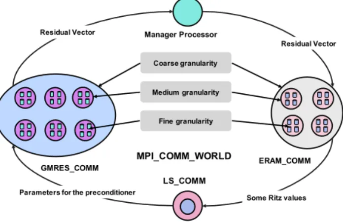
UCGLE method is a distributed parallel method which can profit both shared memory and distributed memory of computational architectures. As shown in Figure 2, it has two levels of parallelism for distributed memory: 1) Coarse Grain/Component level: UC-GLE allows the distribution of different numerical components, including the preconditioning part (LS and ERAM) and the solv-ing part (GMRES) on different platforms or processors; 2) Medium Grain/Intra-component level, GMRES and ERAM components are both deployed in parallel; the third level for shared memory is the Fine Grain/Thread parallelism: the OpenMP thread level paral-lelism in CP U, or the accelerator level paralparal-lelism if GP Us or other accelerators are available.
The GMRES method has been implemented by PETSc, and the ERAM method is provided by SLEPc. Additional functions have been added to the GMRES and ERAM provided by PETSc and SLEPc in order to include the sending and receiving functions of different types of data. For the implementation of LS Component, it computes the convex hull and the ellipse encircling the Ritz values of matrix A, which allows generating a novel Gram matrix M of selected Chebyshev polynomial basis. This matrix should be factorized into LLT by the Cholesky algorithm. The Cholesky method is ensured by PETSc as a preconditioner but can be used as a factorization method. The implementation based on these libraries allows the recompilation of the UCGLE codes to adapt into both CP U and GP U architectures. The experimentation of this paper does not consider the OpenMP thread level of parallelism since the implementation of PETSc and SLEPc is not thread-safe due to their complicated data structures. The data structures of PETSc and SLEPc makes it more
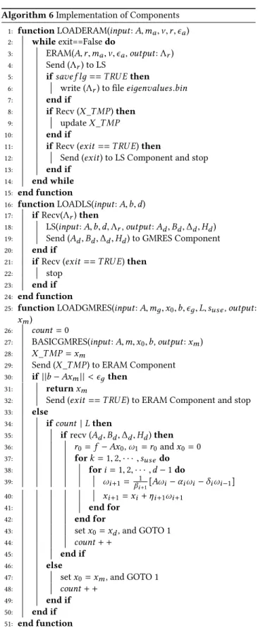
Algorithm 6 Implementation of Components
1: function LOADERAM(input: A,ma, ν, r, ϵa)
2: while exit==False do
3: ERAM(A, r,ma, ν, ϵa,output: Λr)
4: Send (Λr) to LS
5: ifsave f lд == TRU E then
6: write (Λr) to fileeiдenvalues.bin
7: end if
8: if Recv (X _T MP) then 9: updateX _T MP
10: end if
11: if Recv (exit == TRU E) then
12: Send (exit) to LS Component and stop
13: end if 14: end while 15: end function
16: function LOADLS(input: A,b,d) 17: if Recv(Λr)then
18: LS(input: A,b,d, Λr,output: Ad, Bd, ∆d, Hd)
19: Send (Ad, Bd, ∆d, Hd) to GMRES Component
20: end if
21: if Recv (exit == TRU E) then
22: stop
23: end if 24: end function
25: function LOADGMRES(input: A,mд, x0,b, ϵд, L, suse,output:
xm)
26: count = 0
27: BASICGMRES(input: A,m, x0,b, output: xm) 28: X _T MP = xm
29: Send (X _T MP) to ERAM Component
30: if ||b − Axm||< ϵдthen 31: returnxm
32: Send (exit == TRU E) to ERAM Component and stop
33: else 34: ifcount | L then 35: if recv (Ad, Bd, ∆d, Hd)then 36: r0= f − Ax0,ω1= r0andx0= 0 37: fork = 1, 2, · · · ,suse do 38: fori = 1, 2, · · · ,d − 1 do 39: ωi+1= 1
βi+1[Aωi−αiωi −δiωi−1]
40: xi+1= xi+ ηi+1ωi+1
41: end for 42: end for
43: setx0= xd, and GOTO 1 44: count + +
45: end if
46: else
47: setx0= xm, and GOTO 1 48: count + +
49: end if 50: end if 51: end function
ERAM_COMM GMRES_COMM LS_COMM Manager Processor Residual Vector MPI_COMM_WORLD Residual Vector
Some Ritz values Parameters for the preconditioner
Coarse granularity
Medium granularity
Fine granularity
Figure 2: Communication and different levels parallelism of UCGLE method
difficult to partition the data among the threads to prevent conflict and to achieve good performance [3].
The main characteristic of UCGLE method is its asynchronous communication. But the synchronous communication takes place inside of GMRES and ERAM components. Distributed and parallel communication involves different types of exchange data, such as vectors, scalar tables, and signals among different components. When the data are sent and received in a distributed way, it is essential to ensure the consistency of data. In our case, we choose to introduce an intermediate node as a proxy to carry out only several types of exchanges, and thus facilitate the implementation of asynchronous communication. This proxy is calledManager Process as in Figure 2. One process can fulfill all the data exchanges. Asynchronous communication allows each computation com-ponent to conduct independently the work assigned to it without waiting for the input data. The asynchronous data sending and receiving operations are implemented by the non-blocking commu-nication of Message Passing Interface (MPI). Sending takes place after the sender has completed the task assigned to it. Before any prior shipment, the component checks whether several transactions are now on the way. If yes, this task will be canceled to avoid the competition of different types of sending tasks. Sent data are copied into a buffer to prevent them from being modified while sending. For the asynchronous data receiving, before starting this task, the component will check if data is expected to be received. Once the receiving buffer is allocated, the component performs the receiving of data while respecting the distribution of data globally according to the rank of sending processes. It is also important to validate the consistency of receiving data before any use of them by the tasks assigned to the components.
From a view of asynchronous communication, the implementa-tion of UCGLE is to establish of several communicators inside of MPI_COMM_W ORLD and their inter-communication. The topol-ogy of communication among these groups is a circle shown in Figure 2. The total number of computing units supplied by the user is thus divided into four groups according to the following distribu-tion:Ptis the total number of processes, thenPt= Pд+Pa+Pl+Pm,
wherePдis the number of processes assigned to GMRES Compo-nent,Pa the number of processes to ERAM component,Pl the number of processes allocated to LS Component andPf the num-ber of processes allocated toManaдerProcess proxy. PдandPaare greater than or equal to 1,PlandPmare both exactly equal to 1. LS Component is a serial component because the Least Squares polynomial method cannot be parallelized.
Ptis thus divided into several MPI groups according to a color code. The minimum number of processes that our program requires is 4. We utilize the mechanism of MPI standard to fully support the communication of our application. The communication layer that does not depend on the application, this allows the replacement and scalability of various components provided.
3.3
Reusability Analysis
In this section, we study the potential reusability of UCGLE method, which is assured by its asynchronous communication. Indeed, the eigenvalues are used to improve the convergence rate of linear systems by GMRES method. These eigenvalues approximated by ERAM Component can be saved into a local file. For the next time of a different linear system with the same operator matrix, these eigenvalues can be directly reloaded from the local file by LS Com-ponent and execute the preconditioning procedure. This reusability proposes also a new strategy of resolving a series of linear systems in sequence with the same matrix and different right-hand sides. This type of multiple resolving linear systems is well needed in var-ious scientific fields. This strategy is similar to a traditional GMRES method using the Least Squares polynomial method as a deflated preconditioner. But the LS Component and GMRES Component communication keeps asynchronous, thus the preconditioning on the restarted GMRES can be flexible, we can control the frequency of preconditioning and restart (the parameterL). In the experiments, we can propose an autotuning strategy to get an optimizedL for specific linear systems.
It seems if we compute a specific number of eigenvalues before the first time computation and then load them for all the resolving procedures with the same matrix, ERAM component will be not needed, and the existence of UCGLE method will be questioned. In fact, the speedup of UCGLE method depends on the quality and quantity of approximated eigenvalues which cannot always be quickly approximated. The more eigenvalues are calculated, the more accurate these eigenvalues are, the more significant the acceleration of LS preconditioning will be. The multiple solving different linear systems with the same matrix by UCGLE allows the augmentation of eigenvalues number and the amelioration of these values. The reusability of UCGLE method will be presented in future as the page limitation of this article.
3.4
Fault Tolerance Analysis
One important property of the asynchronous UCGLE algorithm is its fault tolerance. That means, the loss of either GMRES Compo-nent or ERAM CompoCompo-nent at run time doesn’t impede the whole computation.
To be more precise:
1) If ERAM computing units are in fault, GMRES Component can continue to run as a classic GMRES method without receiving
Method to Solve Large Scale Non-Hermitian Linear Systems HPC Asia 2018, January 28–31, 2018, Chiyoda, Tokyo, Japan
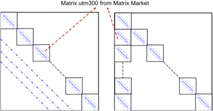
Matrix utm300 from Matrix Market
Figure 3: Two strategies of large and sparse matrix generator by a original matrix utm300 of Matrix Market
the eigenvalues from ERAM Component and the acceleration of LS algorithm.
2) If GMRES computing units are in fault, the fault tolerance mechanism will be more complex. In this situation, firstly the tasks of ERAM Component will be canceled, secondly, these released computing units will be reset as a GMRES Component to continue the resolving procedure without acceleration. The feasibility of replacing ERAM by GMRES is guaranteed. The required materials to retake the resolving task is the operator matrixA, the right-hand sideb and the temporary solution xm. The two former ones have been loaded along with the set-up of UCGLE method. Thexmis ensured to be on the former ERAM computing units since it can be sent and received by the asynchronous communication between GMRES and ERAM Components.
The simulation of ERAM and GMRES Components’ fault toler-ance will be given in Section 4.5.
4
EVALUATION
In this section, we evaluate the acceleration of convergence and the scaling performance of UCGLE method comparing with selected classic preconditioners using the four selected large-scale matrices on both CP U and GP U platforms.
4.1
Hardwares
In experiments, we implement UCGLE method on a cluster ROMEO. ROMEO is located at University of Reims Champagne-Ardenne of France. It is a heterogeneous system made of Xeon CP Us and Nvidia GP Us, with 130 BullX R421 nodes, each node composes 2 processors Intel Ivy Bridge 8 cores @ 2.6 GHz, 2 NVIDIA Tesla K20X accelerators, and 32 GB DDR memory. The exact information of ROMEO is given in Table 1.
4.2
Test Sparse Matrices
UCGLE method has been tested with different matrices, both indus-trial and generated. Our purpose is to test this algorithm on large sparse linear systems. We have successfully evaluated UCGLE with a number of sparse matrices from Matrix Market. However, these matrices are small compared to the desired sizes. Thus we proposed a matrix generator to create several large-scale linear systems. Ad-ditionally, the speedup of UCGLE method depends on the spectrum
Table 1: Node Specifications of the cluster ROMEO
Nodes Number BullX R421× 130 Mother Board SuperMicro X9DRG-QF
CP U Intel Ivy Bridge 8 cores 2,6 GHz× 2 sockets Memory DDR 32GB
GP U NVIDIA Tesla K20X× 2 Memory GDDR5 6 GB / GP U
1 2 4 8 16 32 64 128 256
CPU core or GPU count
10−3 10−2 10−1 100 101
T
im
e
(s
)
Sum operation (CPU) Dot Product operation (CPU)
Sum operation (GPU) Dot product operation (GPU)
Figure 4: Global synchronous communication evaluation by parallel sum and dot product operations on ROMEO; X-axis refers respectively to the CPU core number from 1 to 256 and the GPU core number from 2 to 128; Y-axis refers to the operation time; a base 10 logarithmic scale is used for Y-axis and a base 2 logarithmic scale is used for X-axis.
of linear systems. We have used our scientific large-scale matrices with known eigenvalues to test the UCGLE method.
4.2.1 Matrix Generation. We developed this parallel sparse ma-trix generator based on MPI and PETSc, which reads an industrial matrix of Matrix Market collection as an initial one to build larger ones. This generator allows building a new matrixA by performing several copies of a same small unsymmetrical matrixB onto the diagonal. In order to keep the generated matrices being unsymmet-rical and especially non-block in diagonal, we propose two different strategies to add the values on the off-diagonal ofA, as shown in the Figure 3, the first one is calledML type matrix, and the second is calledMB type matrix. The reason of adding different values on the off-diagonal is to ensure that the eigenvalues of newly generated matrix won’t be the same as the original one, and the convergence rate won’t be too fast.
For the generation of matrixML, several parallel lines with dif-ferent values can be added to the off-diagonal. The good selection
0 500 1000 1500 2000 Iteration Steps 1e-10 1e-8 1e-6 1e-4 1e-2 1 R es id u a l Fault Points Fault Points (a) matLine
SOR Jacobi No preconditioner UCGLE FT(G) UCGLE FT(E) UCGLE
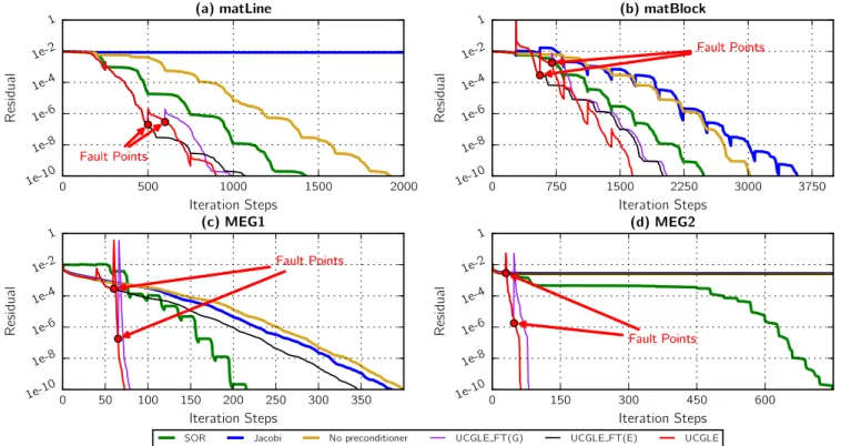
0 750 1500 2250 3000 3750 Iteration Steps 1e-10 1e-8 1e-6 1e-4 1e-2 1 R es id u a l Fault Points Fault Points (b) matBlock 0 50 100 150 200 250 300 350 Iteration Steps 1e-10 1e-8 1e-6 1e-4 1e-2 1 R es id u a l Fault Points Fault Points (c) MEG1 0 150 300 450 600 Iteration Steps 1e-10 1e-8 1e-6 1e-4 1e-2 1 R es id u a l Fault Points Fault Points (d) MEG2
Figure 5: Convergence comparison ofmatLine, matBlock, MEG1 and MEG2 by UCGLE, classic GMRES, Jacobi preconditoned GMRES, SOR preconditioned GMRES, UCGLE_FT(G) and UCGLE_FT(E); X-axis refers to the iteration step for each method; Y-axis refers to the residual, a base 10 logarithmic scale is used for Y-axis; GMRES restarted parameters formatLine, matBlock, MEG1, MEG2 are respectively 250, 280, 30 and 40; ERAM fault points are respectively 500, 560, 60,30, and GMRES fault points are 600, 700, 70 and 48.
Table 2: Test matrices information
Matrix Name n nnz Matrix Type matLine 1.8 × 10⁷ 2.9 × 10⁷ non-Symmetric matBlock 1.8 × 10⁷ 1.9 × 10⁸ non-Symmetric MEG1 1.024 × 10⁷ 7.27 × 10⁹ non-Hermitian MEG2 5.1 × 10⁶ 3.64 × 10⁹ non-Hermitian
of added values can prevent the generated matrix to converge fast with the basic iterative solvers. The way to generate theMB type matrix is much easier, the original matrix is copied on the diagonal and the first block column matrix as shown in the Figure 3.
4.2.2 Test matrices. We have selected four different matrices to evaluate UCGLE method. The matrixmatLine is a ML type matrix, andmatBlock is a MB type matrix, they are both generated by the industrial matrixutm300 which can be downloaded from the Matrix Market. The distribution of eigenvalues in the complex plane has an important impact on the convergence of linear systems. We have selected two scientific matrices with known eigenvalues:MEG1 andMEG2. The eigenvalues of the matrix MEG1 and MEG2 have different eigenvalues distribution in the complex plane. The Table 2 gives the details of these test matrices.
4.3
Global Communication Evaluation
In the parallel algorithms, often one must synchronize the com-munication. The parallel computation of dot product and the sum reduction are the good examples. Synchronization is needed for the execution of these operations. Before the test of UCGLE method, we evaluate the global synchronous communication of both homo-geneous and heterohomo-geneous architecture platforms by the parallel operations of sum and dot product with a real array of size 1.0 × 10⁹. In Figure 4, we can conclude that these global reductions will lose its good scalability if the computing unit number is larger than 64, although ROMEO platform has only hundreds of cores. It can be predicted that this situation will be much worse on the com-ing exascale platforms. In this background, UCGLE is proposed to promote local communication and reduce global synchronous communication.
4.4
Convergence Evaluation
We evaluate the convergence acceleration of four large-scale matri-cesmatLine, matBlock, MEG1, MEG2 using different methods: 1) UCGLE, 2) restarted GMRES without preconditioning, 3) restarted GMRES with SOR preconditioner, 4) restarted GMRES with Jacobi preconditioner. We select the Jacobi and SOR preconditioners for the experimentations because they two are well implemented in
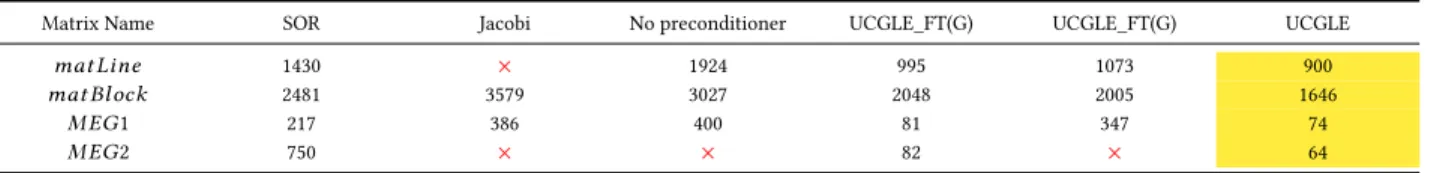
Method to Solve Large Scale Non-Hermitian Linear Systems HPC Asia 2018, January 28–31, 2018, Chiyoda, Tokyo, Japan Table 3: Summary of iteration number for convergence of 4 test matrices using SOR, Jacobi, non preconditioned GM-RES,UCGLE_FT(G),UCGLE_FT(G) and UCGLE: red × in the table presents this solving procedure cannot converge to accurate solution (here absolute residual tolerance 1 × 10⁻¹⁰for GMRES convergence test) in acceptable iteration number (20000 here).
Matrix Name SOR Jacobi No preconditioner UCGLE_FT(G) UCGLE_FT(G) UCGLE
mat Line 1430 × 1924 995 1073 900
mat Block 2481 3579 3027 2048 2005 1646
M EG1 217 386 400 81 347 74
M EG2 750 × × 82 × 64
parallel by PETSc. The GMRES restarted parameter formatLine, matBlock, MEG1, MEG2 are respectively 250, 280, 30 and 40.
Figure 5 compares the convergence curves of experimentation, and the Table 3 gives the convergence steps of each method with 4 test matrices in details. We find that UCGLE method has spectacular acceleration on the convergence rate comparing these conventional preconditioners. It has almost two times of acceleration formatLine, matBlock and MEG1 matrices, and more than 10 times of acceler-ation forMEG2 than the conventional preconditioner SOR. The SOR preconditioner is already much better than the Jacobi precon-ditioner for the test matrices.
4.5
Fault Tolerance Evaluation
The fault tolerance of UCGLE method is also studied by the simula-tion of loss of either GMRES or ERAM Components. UCGLE_FT(G) in Figure 5 represents the fault tolerance simulation of GMRES Com-ponent, and UCGLE_FT(E) implies the fault tolerance simulation of ERAM Component.
The failure of ERAM Component is simulated by fixing the exe-cution loop number of ERAM algorithm, in this case, ERAM exits after a fixed number of solving procedures. We mark the ERAM fault points of four matrices in Figure 5: respectively 500, 560, 60 and 30 iteration step for each case. The UCGLE_FT(E) curves of four experimentations show that GMRES Component will continue to resolve the systems without LS acceleration. The Table 3 shows that the iteration number is greater than the normal UCGLE method but less than the GMRES method without preconditioning.
The failure of GMRES Component is simulated by setting the allowed iteration number of GMRES algorithm to be much smaller than the needed iteration number for convergence. The values of these four cases are respectively 600, 700, 70 and 48. They are also marked in Figure 5. In this figure, after the quitting of GMRES Component without the finish of its task, ERAM computing units will automatically take over the position of GMRES component. The new GMRES resolving procedure will use the temporary solu-tionxm as a new restarted initial vector received asynchronously from the previous restart procedure of GMRES Component before its failure. In this case, ERAM Component no longer exists, thus the resolving task can be continued as the classic GMRES with-out preconditioning. In Figure 5, the UCGLE_FT(E) curves of four experimentations give the simulation of this case. We can find there’s the difference between UCGLE_FT(E) and UCGLE_FT(G). In UCGLE_FT(G), the new GMRES Component takesxmof pre-vious restart procedure, thus it will repeat the iteration steps of previous restart iterations until the failure of GMRES. Another fact of UCGLE_FT(G) which cannot be concluded from Figure 5, but
can be easily obtained, is that the resolving time will be different if the computing units numbers of previous GMRES and ERAM Components are different.
4.6
Scalability Evaluation
The main concern of preconditioned Krylov methods is the cost of per iteration, because of the global communication and synchro-nization overheads. In order to evaluate the performance of UCGLE method on both CP U and GP U clusters, we evaluate its strong scal-ability comparing with the classic and preconditioned GMRES by the average time cost per iteration. The test matrix isMEG1. The average time cost for these methods is computed by a fixed num-ber of iterations. Time per iteration is suitable for demonstrating scaling behavior.
For the evaluation of UCGLE method on the homogeneous clus-ter, the four computing components are all implemented on the CP Us, the core number of GMRES Component is set respectively to be 1, 2, 4, 8, 16, 32, 64, 128, 256, and both the core number of LS Com-ponent and Manager ComCom-ponent is 1. ERAM ComCom-ponent should ensure to supply the approximated eigenvalues in time for each time restart of GMRES Component, thus the core number is respectively 1, 1, 1, 1, 4, 4, 4, 10, 16, referring to different GMRES Component core number. For the evaluation on the heterogeneous cluster, GM-RES Component and ERAM Component are implemented on GP Us, both LS Component and Manager Component allocate only 1 core on CP U. The GP U number of GMRES Component is set respectively to be 2, 4, 8, 16, 32, 64, 128, with the GP U number of ERAM Compo-nent respectively 1, 1, 1, 4, 4, 4, 8. The computing resource number of classic and preconditioned GMRES keeps always the same with the core number of GMRES Component in UCGLE method, thus it ranges from 1 to 256 for CP U performance evaluation, and from 2 to 128 for GP U performance evaluation.
In the experimentations, firstly we can find that UCGLE method is able to take advantages of the GP U accelerators which has almost 4 times speed up for the time cost per iteration comparing with the homogenous cluster without accelerators.
In Figure 6, we can find that these methods have good scalabil-ity both on CP U and GP U with the augmentation of computing units except the SOR preconditioned GMRES. The classic GMRES has smallest time cost per iteration. The Jacobi preconditioner is the simplest preconditioning form for GMRES. This time cost gap between Jacobi preconditioned GMRES and classic GMRES is not enormous. The GMRES with SOR preconditioner has the largest time cost per iteration since SOR preconditioned GMRES has the additional matrix-vector and matrix-matrix multiplication opera-tions in each step of the iteration. These operaopera-tions have global
1 2 4 8 16 32 64 128 256
GMRES CPU core or GPU count
10−2 10−1 100 101 102 T im e (s ) SOR (CPU) Jacobi (CPU) No preconditioner (CPU) UCGLE (CPU) SOR (GPU) Jacobi (GPU) No preconditioner (GPU) UCGLE (GPU)
Figure 6: Strong scalability test of solve time per iteration for UCGLE, GMRES without preconditioner, Jacobi and SOR preconditioned GMRES using matrix MEG1 on CPU and GPU; X-axis refers respectively to CPU cores of GMRES from 1 to 256 and GPU number of GMRES from 2 to 128; Y-axis refers to the average execution time per iteration. A base 2 logarithmic scale is used for X-axis, and a base 10 log-arithmic scale is used for Y-axis.
communication and synchronization points. The communication overhead makes the SOR preconditioned GMRES much more eas-ily lose its good scalability with the augmentation of computing unit number. There isn’t much difference between the time cost per iteration of classic GMRES and UCGLE. This phenomenon is caused by the asynchronous communication of UCGLE method. Since the resolving part and preconditioning part of UCGLE work independently, the global communication and synchronize points of UCGLE is similar with the classic GMRES for each time of pre-conditioning. That’s the benefits of UCGLE and its asynchronous communication.
4.7
Performance Evaluation
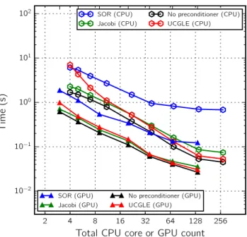
The average time cost per iteration is also used to evaluate their performance. For the performance comparison, it is necessary to keep the total computing resource number of UCGLE and other methods the same. We have tested the classic and conventional pre-conditioned GMRES with the CP U core number fixed respectively as 4, 5, 7, 11, 22, 38, 70, 140, 274 and the GP U number fixed respec-tively as 3, 5, 9, 20, 36, 68, 136, referring to the previous evaluation of UCGLE method in Section 4.6. In the evaluation on GP U cluster, the two CP Us for LS Component and Manager Component have been ignored because they have a minor influence.
The performance comparison is given in Figure 7. We can find that if the computing resource number is small, the performance of classic and conventional preconditioned GMRES is much better
2 4 8 16 32 64 128 256
Total CPU core or GPU count
10−2 10−1 100 101 102 T im e (s ) SOR (CPU) Jacobi (CPU) No preconditioner (CPU) UCGLE (CPU) SOR (GPU) Jacobi (GPU) No preconditioner (GPU) UCGLE (GPU)
Figure 7: Performance comparison of solve time per itera-tion for UCGLE, GMRES without precondiitera-tioner, Jacobi and SOR preconditioned GMRES using matrixMEG1 on CPU and GPU; X-axis refers respectively to the total CPU cores num-ber or GPU numnum-ber for these four methods; Y-axis refers to the average execution time per iteration. A base 2 logarith-mic scale is used for X-axis, and a base 10 logarithlogarith-mic scale is used for Y-axis.
than UCGLE since the latter allocates extra computing resources for other components. With the augmentation of computing resources, if the CP U core number is larger than 22 or the GP U number is larger than 5, it comes that the etra computing ressources have slight influence on the resolution, and the average time cost per it-eration of UCGLE method trends to be similar to the ones of classic GMRES, and to be much better than the conventional precondi-tioned, especially the SOR preconditioned GMRES. For test matrix MEG1, UCGLE method has similar speedup on the solving time per iteration comparing with the classic GMRES when the computing resource number is larger than 22 for CP Us and larger than 5 for GP Us, but it can decrease significantly more than 5× iteration step number for the convergence, thus about 5× acceleration for the time of the whole resolution. In the end, the better performance of UCGLE method comparing with other methods can be concluded.
5
CONCLUSION AND PERSPECTIVES
In this paper, we have presented a distributed and parallel method UCGLE for solving large-scale non-Hermitian linear systems. This method has been implemented with asynchronous communication among different computation components. In the experimentation, we observed that UCGLE method has following features: 1) it has significant acceleration for the convergence than the conventional preconditioners as SOR and Jacobi; 2) the spectrum of different lin-ear systems has influence on its improvement of convergence rate; 3) it has better scalability for the very large-scale linear systems;
Method to Solve Large Scale Non-Hermitian Linear Systems HPC Asia 2018, January 28–31, 2018, Chiyoda, Tokyo, Japan 4) it is able to speed up using GP Us; 5) it has the fault tolerance
mechanism facing the failure of different computation components. We conclude that UCGLE method is a good candidate for emerg-ing large-scale computational systems because of its asynchronous communication scheme, its multi-level parallelism, its reusability and fault tolerance and its potential load balancing. The coarse grain parallelism among different computation components and the medium/fine grain parallelism inside each component can be flexibly mapped to large-scale distributed hierarchical platforms.
Various parameters have an impact on the convergence. Thus, an auto-tuning is required in the future work, where the systems can select different Krylov subspace dimensions, numbers of eigenval-ues to be computed, degrees of Least Squares polynomial according to different linear systems and cluster architectures.
PETSc and SLEPc are not well compatible with the Intel Xeon Phi architectures. Additionally, other hybrid methods can be proposed with different computing components using unite and conquer ap-proach, but it is difficult to implement them without the knowledge of MPI communication. YvetteML (YML) [7] is a workflow language based on user-friendly and hierarchical system-oriented develop-ment and execution environdevelop-ment, and XcalableMP (XMP) [14] is a directive-based language extension for distributed memory sys-tems. With YML, the user can automatically allocate the computing units and establish the inter-communication for different tasks. It is necessary to develop a new version of UCGLE method with this multi-level languages YML-XMP for various architectures.
ACKNOWLEDGMENTS
The authors would like to thank ROMEO HPC Center-Champagne Ardenne for their support in provinding the use of clusterROMEO. This work is supported by the projectMYX of French National Research Agency (ANR) with the project ID: ANR-15-SPPE-003.
REFERENCES
[1] Tofigh Allahviranloo. 2005. Successive over relaxation iterative method for fuzzy system of linear equations.Appl. Math. Comput. 162, 1 (2005), 189–196. [2] Walter Edwin Arnoldi. 1951. The principle of minimized iterations in the solution
of the matrix eigenvalue problem.Quarterly of applied mathematics 9, 1 (1951), 17–29.
[3] Satish Balay, Shrirang Abhyankar, Mark F. Adams, Jed Brown, Peter Brune, Kris Buschelman, Lisandro Dalcin, Victor Eijkhout, William D. Gropp, Dinesh Kaushik, Matthew G. Knepley, Lois Curfman McInnes, Karl Rupp, Barry F. Smith, Stefano Zampini, Hong Zhang, and Hong Zhang. 2016. PETSc Users Manual. Technical Report ANL-95/11 - Revision 3.7. Argonne National Laboratory. http: //www.mcs.anl.gov/petsc
[4] Claude Brezinski and M Redivo-Zaglia. 1994. Hybrid procedures for solving linear systems.Numer. Math. 67, 1 (1994), 1–19.
[5] SH Chan, KK Phoon, and FH Lee. 2001.A modified Jacobi preconditioner for solving ill-conditioned Biot’s consolidation equations using symmetric quasi-minimal residual method. International Journal for Numerical and Analytical Methods in Geomechanics 25, 10 (2001), 1001–1025.
[6] Edmond Chow and Yousef Saad. 1997. Experimental study of ILU preconditioners for indefinite matrices.J. Comput. Appl. Math. 86, 2 (1997), 387–414. [7] Olivier Delannoy, FranceNahid Emad, and Serge Petiton. 2006. Workflow global
computing with yml. InProceedings of the 7th IEEE/ACM International Conference on Grid Computing. IEEE Computer Society, 25–32.
[8] Jack Dongarra, Jeffrey Hittinger, John Bell, Luis Chacon, Robert Falgout, Michael Heroux, Paul Hovland, Esmond Ng, Clayton Webster, and Stefan Wild. 2014. Applied mathematics research for exascale computing. Technical Report. Lawrence Livermore National Laboratory (LLNL), Livermore, CA.
[9] Nahid Emad and Serge Petiton. 2016. Unite and conquer approach for high scale numerical computing.Journal of Computational Science 14 (2016), 5–14. [10] Nahid Emad, Serge Petiton, and Guy Edjlali. 2005. Multiple explicitly restarted
Arnoldi method for solving large eigenproblems. SIAM Journal on Scientific Computing 27, 1 (2005), 253–277.
[11] Jocelyne Erhel, Kevin Burrage, and Bert Pohl. 1996. Restarted GMRES precon-ditioned by deflation.Journal of computational and applied mathematics 69, 2 (1996), 303–318.
[12] Alexandre Fender, Nahid Emad, Serge Petiton, and Joe Eaton. 2016. Leveraging accelerators in the multiple implicitly restarted Arnoldi method with nested subspaces. InEmerging Technologies and Innovative Business Practices for the Transformation of Societies (EmergiTech), IEEE International Conference on. IEEE, 389–394.
[13] David S Kershaw. 1978. The incomplete Cholesky conjugate gradient method for the iterative solution of systems of linear equations.J. Comput. Phys. 26, 1 (1978), 43–65.
[14] Jinpil Lee and Mitsuhisa Sato. 2010. Implementation and performance evaluation of xcalablemp: A parallel programming language for distributed memory systems. InParallel Processing Workshops (ICPPW), 2010 39th International Conference on. IEEE, 413–420.
[15] Richard B Lehoucq and Danny C Sorensen. 1996. Deflation techniques for an implicitly restarted Arnoldi iteration.SIAM J. Matrix Anal. Appl. 17, 4 (1996), 789–821.
[16] Thomas A Manteuffel. 1977. The Tchebychev iteration for nonsymmetric linear systems.Numer. Math. 28, 3 (1977), 307–327.
[17] Youcef Saad. 1984. Chebyshev acceleration techniques for solving nonsymmetric eigenvalue problems.Math. Comp. 42, 166 (1984), 567–588.
[18] Youcef Saad. 1987.Least squares polynomials in the complex plane and their use for solving nonsymmetric linear systems.SIAM J. Numer. Anal. 24, 1 (1987), 155–169.
[19] Yousef Saad. 2011.Numerical Methods for Large Eigenvalue Problems: Revised Edition. SIAM.
[20] Youcef Saad and Martin H Schultz. 1986. GMRES: A generalized minimal residual algorithm for solving nonsymmetric linear systems.SIAM Journal on scientific and statistical computing 7, 3 (1986), 856–869.
[21] Yousef Saad, Manshung Yeung, Jocelyne Erhel, and Frédéric Guyomarc’h. 2000. A deflated version of the conjugate gradient algorithm.SIAM Journal on Scientific Computing 21, 5 (2000), 1909–1926.
[22] Gerard LG Sleijpen and Diederik R Fokkema. 1993. BiCGstab (l) for linear equations involving unsymmetric matrices with complex spectrum.Electronic Transactions on Numerical Analysis 1, 11 (1993), 2000.