Quantum coherence in the integer quantum Hall regime

HAL Id: tel-00348151

https://tel.archives-ouvertes.fr/tel-00348151v2

Submitted on 3 Jan 2010

HAL is a multi-disciplinary open access

archive for the deposit and dissemination of sci-entific research documents, whether they are pub-lished or not. The documents may come from teaching and research institutions in France or abroad, or from public or private research centers.

L’archive ouverte pluridisciplinaire HAL, est destinée au dépôt et à la diffusion de documents scientifiques de niveau recherche, publiés ou non, émanant des établissements d’enseignement et de recherche français ou étrangers, des laboratoires publics ou privés.

Preden Roulleau

To cite this version:

Preden Roulleau. Quantum coherence in the integer quantum Hall regime. Condensed Matter [cond-mat]. Université Pierre et Marie Curie - Paris VI, 2008. English. �tel-00348151v2�

THESE

pr´esent´ee le 19 novembre 2008 pour l’obtention du

Doctorat de l’Universit´e Pierre et Marie Curie - Paris 6

Sp´ecialit´e Physique Quantique

par

Preden ROULLEAU

Etude de la coh´

erence quantique

dans le r´

egime d’effet Hall quantique

entier

Composition du jury Rapporteurs : Markus Buttiker

Marc Sanquer Examinateurs : Moty Heiblum

Klaus Ensslin Benoˆıt Doucot Directeurs de th`ese : D. Christian Glattli

Patrice Roche

Table des mati`

eres

1 Remerciements 6

2 R´esum´e de la th`ese 8

2.1 Introduction . . . 8

2.2 Montage exp´erimental . . . 10

2.3 Visibilit´e `a tension finie . . . 12

2.4 Longueur de coh´erence phase `a facteur de remplissage 2 (ν = 2) . . . . 14

2.5 Origine de la longueur de coh´erence de phase finie . . . 14

2.6 ”Voltage Probe” . . . 17

3 Introduction 19 3.1 Toward Bell’s inequality in mesoscopic physics . . . 20

3.1.1 Definition of the entanglement . . . 20

3.1.2 EPR Paradox and Bell’s inequality . . . 20

3.1.3 Violation of the Bell’s inequality . . . 22

3.2 Electronic entanglement in the two-particle interferometer . . . 22

3.3 From the simple Mach Zehnder Interferometer to the two-particle interfero-meter . . . 25

3.3.1 The two-particle Aharonov-Bohm effect . . . 25

3.3.2 Technical realization . . . 28

3.4 Conclusion . . . 28

4 The electronic MZI 30 4.1 Introduction . . . 31

4.2 From optics to mesoscopic physics : description of the optical MZI . . . 31

4.3 An electronic beam : the edge state of the Integer Quantum Hall regime . . 33

4.3.1 The classical Hall effect . . . 33

4.3.2 The quantum Hall effect . . . 34

4.3.3 Electrons without spin . . . 35

4.3.4 Electrons with spin . . . 36

4.3.5 Hall resistance and Shubnikov-de-Haas oscillations . . . 36

4.3.6 Edge states . . . 37

4.4 Electronic Beam Splitter : the Quantum Point Contact . . . 39

4.4.1 The Quantum Point contact . . . 40

4.5 The electronic Mach Zehnder Interferometer . . . 41

4.5.1 Description . . . 41

4.5.2 Fabrication process . . . 42

4.5.3 The two dimensional electron gas . . . 42

4.5.4 Aharonov Bohm oscillations . . . 43

4.6 Experimental technics . . . 44

4.6.1 Conductance measurements . . . 44

4.6.2 Noise measurements . . . 45

4.6.3 Measuring the visibility in the MZI . . . 47

4.7 Conclusion . . . 50

5 Finite bias visibility 54 5.1 Introduction . . . 55

5.2 Unexpected behavior of the visibility at finite bias . . . 55

5.2.1 The very first experiment : a monotonous decrease . . . 56

5.2.2 One channel biased : an unexpected lobe pattern . . . 56

5.3 General properties of the lobe structure . . . 57

5.3.1 Magnetic field dependence . . . 57

5.3.2 Dependence on the dilution . . . 59

5.3.3 Two channels biased . . . 60

5.4 Our experimental results . . . 62

5.4.1 Phase rigidity and visibility . . . 62

5.4.2 A Gaussian shape visibility . . . 64

5.4.3 Influence of the dilution . . . 66

5.5 Coupling between the inner and outer edge state . . . 68

5.5.1 Modelling the capacitive coupling between edge states . . . 68

5.6 Discussion regarding the visibility . . . 72

5.6.1 Only one edge channel is biased . . . 72

5.6.2 Two edge states are biased . . . 74

5.6.3 The lobe eraser . . . 77

5.6.4 The lobe width : comparison between the inner and outer edge state 78 5.7 Theoretical approach . . . 79

5.7.1 The non interacting model . . . 79

5.7.2 Interaction between counterpropagating edge states . . . 81

5.7.3 Short range interactions . . . 81

5.8 Shot noise generated by the first beam splitter . . . 84

5.8.1 Discussion of this model . . . 85

5.8.2 An asymmetric configuration . . . 85

6 The Coherence Length at ν=2 94

6.1 Introduction . . . 94

6.2 Methodology . . . 95

6.3 Determination of lϕ . . . 98

6.3.1 Temperature dependence . . . 99

6.4 Phase rigidity and absence of thermal smearing . . . 100

6.4.1 Definition of thermal smearing . . . 100

6.4.2 Absence of thermal smearing . . . 101

6.5 Properties of lϕ . . . 102

6.5.1 Determination of lϕ . . . 102

6.5.2 Magnetic field dependence of lϕ . . . 103

6.6 Some universality ? . . . 104

6.7 Conclusion . . . 105

7 Origin of the finite coherence length 111 7.1 Introduction . . . 112

7.2 Coupling an Interferometer to a noisy environment . . . 112

7.2.1 Quantum dot detector . . . 112

7.2.2 Sprinzak et al. experiment . . . 114

7.2.3 Rohrlich et al. experiment . . . 116

7.2.4 A true Which Path experiment ? . . . 117

7.2.5 Proposal with the MZI . . . 118

7.2.6 Optical experiment . . . 118

7.3 Inner and outer edge state coupling . . . 120

7.3.1 Characterizing the coupling . . . 121

7.3.2 Magnetic field dependence of the coupling parameter . . . 121

7.3.3 Gaussian Noise dephasing . . . 124

7.3.4 The Gaussian approximation . . . 125

7.3.5 The magnetic field dependence . . . 127

7.4 An explanation to the finite coherence length . . . 128

7.4.1 Impact of the inner edge state . . . 128

7.4.2 An approach valid on the whole plateau ν = 2 . . . 129

7.5 Non-Gaussian noise . . . 130

7.6 Theory : Finite frequency coupling . . . 133

7.6.1 The capacitive coupling . . . 133

7.6.2 Admittance matrix and noisy inner edge state . . . 134

7.6.3 Screening of fluctuations . . . 136

7.7 Conclusion . . . 138

8 The Voltage Probe 144 8.1 Introduction . . . 144

8.2 Ohmic contact detector . . . 145

8.2.2 A specific design . . . 146

8.2.3 Phase evolution . . . 147

8.3 Study of a resonance . . . 148

8.3.1 Effect of a resonance on the phase . . . 149

8.3.2 Modelling the resonance . . . 149

8.4 Decoherence and Phase averaging . . . 151

8.4.1 Decoherence in the MZ : the voltage probe approach . . . 152

8.5 Conclusion . . . 155

9 Conclusion 160 10 R´esum´e/Abstract 162 10.1 R´esum´e . . . 162

10.2 Abstract . . . 163

A The Landauer Buttiker formalism 164 A.1 Quantum of conductance . . . 164

A.1.1 Landauer formula for a monomode conductor . . . 165

A.1.2 2D systems . . . 167

B Admittance matrix 169 C Expression of U1 in function of V2 173 C.1 Notations . . . 173

C.2 Low frequency limit . . . 174

Chapitre 1

Remerciements

Ces trois ann´ees de th`ese `a Saclay ont ´et´e pour moi trois belles ann´ees. J’y ai d´ecouvert le m´etier de chercheur avec ses moments de doutes quand ” tout fout le camp ”, et ses moments ” magiques ” lorsque la nature r´ev`ele enfin ses secrets.

Cette aventure n’aurait pas ´et´e possible sans la direction de Patrice Roche. Patrice m’a d’abord enseign´e la rigueur scientifique. Il a toujours pris soin de m’expliquer la physique m´esoscopique dans ses moindres d´etails, et nos discussions ont ´et´e d’une grande richesse scientifique. Il a aussi ´et´e un encadrant exceptionnel qui m’a toujours soutenu dans les p´eriodes les plus dures, qui a corrig´e avec tact mes principaux d´efauts tout en valorisant mes qualit´es.

J’ai d´ecouvert la physique m´esoscopique grˆace `a Christian Glattli. C’est lui qui a jet´e les bases de ce qui deviendra pour moi une r´ev´elation. Christian a toujours ´et´e `a mon ´ecoute pendant ses trois ann´ees et j’ai pu b´en´eficier de sa connaissance profonde de la physique m´esosopique.

Fabien Portier et Xavier Waintal ont ´et´e d’un grand soutien pendant cette th`ese. Fabien d´eborde d’id´ees et nos ´echanges scientifiques ont ´et´e extrˆemement fructueux. Xavier, mˆeme s’il n’a pas directement ´et´e impliqu´e dans l’exp´erience m’a ´eclair´e sur les subtilit´es du ” champ ” scientifique. Xavier a aussi ´et´e un partenaire de randori exceptionnel quasi quotidien (en g´en´eral apr`es la pause d´ejeuner, conf´erences inclues).

Toutes ces exp´eriences r´ealis´ees sur le Mach Zehnder n’auraient pas ´et´e possibles sans les ” golden hands ” du LPN : Dominique Mailly et GianCarlo Faini. La difficult´e de ces exp´eriences reposait en grande partie sur l’extrˆeme complexit´e de l’´echantillon : j’ai pu b´en´eficier pendant ma th`ese d’une s´erie d’´echantillons exceptionnelle. Dominique Mailly et GianCarlo Faini ont toujours apport´e un angle nouveau `a nos mesures, et notre partenariat fut d’une grande richesse scientifique. Enfin j’aimerais remercier Ulf Gennser pour nous avoir fourni le gaz 2D et pour son aide lors de la relecture des articles.

J’ai eu l’honneur d’avoir dans mon jury de th`ese des grands noms de la physique m´esoscopique. J’ai ´et´e tr`es honor´e de la pr´esence de Moty Heiblum et j’aimerais le remercier d’avoir fait le d´eplacement depuis Israel. Moty Heiblum a ce g´enie de pouvoir d´evoiler la beaut´e de la physique m´esoscopique dans ce qu’elle a de plus simple. J’aimerais ´egalement remercier Markus Buttiker et Marc Sanquer tous deux rapporteurs de ma th`ese, pour la

qualit´e de leurs corrections. J’ai ´et´e tr`es heureux d’avoir dans mon jury Klaus Ensslin. J’aimerais remercier celui qui m’accueille actuellement dans son laboratoire. Enfin, merci `a Benoit Dou¸cot pour avoir ´et´e mon directeur de jury.

Patrice Jacques m’a ´et´e d’une aide pr´ecieuse lors des modifications exp´erimentales. J’ai b´en´efici´e pendant ma th`ese de sa grande connaissance des d´etails technique de l’exp´erience. J’aimerais remercier les th´esards et post docs du groupe nano-´electronique : eva, ge-nevi`eve, keyan, lorentz, julien, valentin, kyril et joseph. Les stagiaires qui ont travaill´e sur l’exp´erience : Brice et Fung Han qui a maintenant repris le flambeau. Merci au groupe quantronique pour leur acceuil toujours tr`es chaleureux. Merci `a Eric Vincent, directeur du SPEC, de m’avoir accueilli dans son laboratoire. Merci `a Patrick Pari et Philippe Forget pour leur gentillesse. Merci a tous ceux qui au SPEC m’ont accompagn´e pendant ces trois ann´ees.

J’aimerais remercier tous les judokas du PUC judo : le judo fut pour moi un pilier essentiel pendant cette th`ese. J’aimerais remercier mes amis : max, val yannick, fx, bob, tim, r´emi, charles, anne, mes parents qui m’ont toujours soutenu, ma soeur marjolaine, et ma famille. Merci `a ce que j’avais de plus pr´ecieux : Marie.

Chapitre 2

R´

esum´

e de la th`

ese

Contents

2.1 Introduction . . . 8 2.2 Montage exp´erimental . . . 10 2.3 Visibilit´e `a tension finie . . . 12 2.4 Longueur de coh´erence phase `a facteur de remplissage 2 (ν = 2) 14 2.5 Origine de la longueur de coh´erence de phase finie . . . 14 2.6 ”Voltage Probe” . . . 17

2.1

Introduction

Figure 2.1 – Repr´esentation sch´ematique du double MZI propos´ee par Samuelsson et al. [74]. Les ´electrons sont inject´es au niveau des contacts 2 et 3, A, B, C et D ´etant des lames s´eparatrices. La mesure de corr´elation ´electronique crois´ee est effectu´ee entre les contacts 5 et 8. φ est la phase accumul´ee le long de chaque trajectoire ´electronique. Par exemple φ1est la phase accumul´ee le long des bords entre les lames

s´eparatrices C et A. La mesure de bruit en corr´elation crois´ee entre les contacts 5 et 8 est sensible `a la phase Aharonov-Bohm `a deux ´electrons : φ = φ1+ φ2− φ3− φ4

L’objectif de cette th`ese est d’observer la violation des in´egalit´es de Bell pour un conducteur m´esoscopique. Le principe g´en´eral s’inspire de l’exp´erience r´ealis´ee en 1982 par Aspect et al [9]. Cette exp´erience a ´et´e propos´ee pour la premi`ere fois en 2004 par Samuelsson et al [74][60]. Nous avons repr´esent´e figure 1 le sch´ema de cette exp´erience appel´e double interf´erom`etre de Mach Zehnder (MZI). Contrairement `a l’exp´erience d’As-pect et al. deux sources ´electroniques distinctes sont utilis´ees (num´erot´ees 2 et 3 sur la figure 2.1). Consid´erons dans un premier temps l’onde ´electronique ´emise par le r´eservoir 2. Elle sera soit transmise soit r´efl´echie par la premi`ere lame s´eparatrice C. Si elle est transmise, elle accumulera la phase φ1 jusqu’`a la prochaine lame s´eparatrice not´ee A. Si

elle est r´efl´echie, elle accumulera la phase φ3 jusqu’`a la prochaine lame s´eparatrice not´ee B.

Consid´erons maintenant l’onde ´electronique ´emise par le r´eservoir 3. Elle sera soit transmise soit r´efl´echie par la premi`ere lame s´eparatrice D. Si elle est transmise, elle accumulera la phase φ2 jusqu’`a la prochaine lame s´eparatrice not´ee A. Si elle est r´efl´echie, elle accumulera

la phase φ4 jusqu’`a la prochaine lame s´eparatrice not´ee B. On effectue ensuite une mesure

de corr´elation ´electronique entre les contacts 5 et 8. La mesure sur le contact 5 ne permet pas de diff´erencier l’´electron ´emis par le r´eservoir 2 de l’´electron ´emis par le r´eservoir 3. On peut donc montrer que la mesure de corr´elation ´electronique va ”s´electionner” la partie intriqu´ee de l’´etat `a deux ´electrons. Cette mesure de la partie intriqu´ee de l’´etat `a deux ´electrons est sensible `a la diff´erence de phase : φ1+φ2-φ3-φ4. Lorsque l’aire d´efinie par ce

chemin ´electronique est soumise `a un champs magn´etique perpendiculaire, on peut faire varier cette diff´erence de phase via le champ magn´etique appliqu´e. La partie intriqu´ee sera r´ev´el´ee par des oscillations Aharonov Bohm dans une mesure `a deux ´electrons, le bruit. Une fois ces oscillations observ´ees, il s’agit de r´egler les diff´erentes lames s´eparatrices afin d’ob-tenir l’´etat maximalement intriqu´e, pour finalement proc´eder `a la violation des in´egalit´es de Bell. 3 5 4 φ 2 φ A C D B 2 3 φ 1 φ 8 SG

Figure 2.2 – Les notations sont similaires `a la figure 1. On note cependant ici la pr´esence d’une lame s´eparatrice centrale (not´ee SG) qui, lorsqu’elle est ferm´ee, s´epare le double MZI en deux simples MZI, de

fa¸con a optimiser les r´eglages (´etant convenu qu’il est plus facile d’obtenir des oscillations Aharonov Bohm `a un ´electron qu’`a deux ´electrons). Une fois cette la lame s´eparatrice ouverte, on retrouve la configuration double MZI.

Exp´erimentalement nous n’appliquerons pas directement la g´eom´etrie propos´ee par Sa-muelsson et al.. On peut montrer[60] que le double MZI peut ˆetre d´ecompos´e en deux MZI simples s´epar´es d’une lame s´eparatrice. Un r´eglage optimal du simple MZI [37] permet

d’observer des oscillations Aharonov Bohm `a un ´electron. Une fois que les deux simples MZI sont r´egl´es afin d’obtenir la visibilit´e maximale, on ouvre le lame s´epatrice centrale pour se retrouver dans la configuration double MZI. Nous allons discuter maintenant des outils m´esoscopiques n´ecessaires `a l’´elaboration d’un MZI ´electronique.

2.2

Montage exp´

erimental

Pour construire un MZI en physique m´esoscopique nous avons besoin de deux ´el´ements : d’un faisceau d’´electrons et de lames s´eparatrices. Pour obtenir un faisceau ´electronique nous travaillerons en r´egime Hall quantique, dans un gaz bidimensionnel(AsGa/GaAlAs). Nous savons en effet qu’en r´egime Hall quantique le transport ´electronique a lieu dans des canaux de bord que l’on peut se repr´esenter comme des conducteurs 1D chiraux. En effet les ´electrons soumis `a un champs magn´etique perpendiculaire ont une trajectoire cyclotron. Si loin des bords la vitesse moyenne des ´electrons est nulle, au bord de l’´echantillon , les ´electrons seront soumis au potentiel de bord. La repr´esentation semi classique que l’on peut se faire de ce ph´enom`ene est montr´ee figure 2.3.

edge states

x y

Semi-classical representation of edge states

Figure 2.3 –Repr´esentation semi classique des canaux de bord en r´egime Hall quantique. La trajectoire des ´electrons dans le bulk peut ˆetre d´ecrite par une trajectoire cyclotron. Le long des bords de l’´echantillon, le centre de l’orbite cyclotron d´erive.

Le long des bords les ´electrons rebondissent et le centre de l’orbite cyclotron d´erive : en moyenne la vitesse de d´erive des ´electrons le long des bords n’est pas nulle. Si l’on consid`ere maintenant l’hamiltonien de l’´electron dans un gaz 2D soumis `a un champ magn´etique per-pendiculaire, on peut montrer que les niveaux d’´energie sont discrets (niveaux de Landau). Lorsque l’on se rapproche des bords de l’´echantillon, les niveaux de Landau vont ˆetre d´eform´es par le potentiel de confinement. Le transport ´electronique aura lieu au croise-ment entre ces niveaux de Landau courb´es et l’´energie de Fermi. Le nombre de canaux de bord est ´egal au nombre de croisements entre niveaux de Landau et ´energie de Fermi. Nos r´esultats ont ´et´e obtenus `a facteur de remplissage 2 (ν=2) : deux niveaux d’´energie

croisent le niveau de Fermi, on travaille avec deux canaux de bord. Pour ce qui est des lames s´eparatrices ´electroniques, les contact ponctuels quantiques (CPQ) sont parfaitement adapt´es. Nous avons repr´esent´e figure 2.4(a) une vue SEM d’un CPQ.

VG

IT

IR

I0

(b)

I

I

I

(a)

Figure 2.4 –(a) Vue SEM d’un CPQ. Une partie de l’onde ´electronique est r´efl´echie (transmise) not´ee

IR (not´ee IT). (b) Vue SEM d’un CPQ dans la partie centrale du MZI. En jaune nous avons repr´esent´e le

pont qui connectent les deux grilles du CPQ, en rouge un contact ohmique connect´e `a la masse. Dans cette repr´esentation, une partie de l’onde ´electronique est transmise vers le deuxi`eme CPQ. La partie r´efl´echie pourra ˆetre collect´ee par le contact `a la masse.

Figure 2.4(b) ce mˆeme CPQ mais int´egr´e dans le MZI : en jaune un pont qui permet de connecter les deux grilles du CPQ. En appliquant une tension n´egative sur le CPQ, on d´epl´ete localement sous le CPQ et on augmente le couplage entre canaux contre propa-geants. On peut ainsi contrˆoler de mani`ere tr`es pr´ecise la probabilit´e de transmission ou de r´eflexion d’une onde ´electronique. Nous avons d´esormais tous les outils pour comprendre le principe g´en´eral du MZI. Nous en avons repr´esent´e une vue SEM figure 2.5.

4 µm I₀ I_T G2 G1 G0 LG I_D (u) (d) IR

Figure 2.5 –Vue SEM du MZI ´electronique. G0, G1 et G2 sont des CPQ qui servent de lames s´epratrices. G0 permet une dilution du courant inject´e, G1 et G2 sont les deux lames s´eparatrices de l’interf´erom`etre. LG est une grille lat´erale qui permet la variation de l’aire de la surface d´efinie par (u) and (d). Le petit contact ohmique central entre les deux bras du MZI permet de collecter le courant r´etrodiffus´e `a la masse grˆace `a un long pont en or.

G1 et G2 sont les deux lames s´eparatrices de l’interf´erom`etre. Lorsqu’il est r´el´echi

en G2. Si on consid`ere maintenant l’approche `a une particule du formalisme Landauer-Buttiker, l’amplitude de transmission t `a travers le MZI est la somme de deux amplitudes de transmission correspondant aux chemins (u) et (d). Pour des amplitudes de transmission et de r´eflexion ti et ri du i`eme CPQ (avec |ri|2+|ti|2=1), l’amplitude de transmission est donn´ee par :

t = t1eiφdt2− r1eiφur2.

o`u φu (φd) est la phase accumul´ee le long du chemin sup´erieur (inf´erieur) . On obtient la probabilit´e de transmission :

T = T1T2+ R1R2+

p

T1T2R1R2sinϕ(²) (2.1)

o`u ϕ(²) = φu − φd et Ti =| ti |2= 1 − Ri. ϕ(²) est le flux du champs magn´etique `a travers l’aire d´efinie par les deux trajetoires `a l’´energie ². On dispose donc de deux mani`eres pour observer les franges d’oscillations : soit en faisant varier le champs magn´etique soit en faisant varier l’aire d´efinie par les deux trajectoires grˆace `a la grille lat´erale (not´ee LG sur la figure 2.5).

2.3

Visibilit´

e `

a tension finie

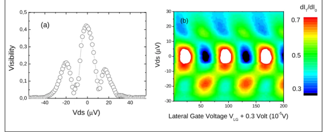
La mesure de bruit en corr´elation crois´ee, pour s´electionner la partie intriqu´ee de l’´etat `a deux ´electrons, se fait `a tension finie. Avant de r´ealiser cette mesure, il s’agit donc de comprendre la visibilit´e1 _{de la conductance `a tension finie. La visibilit´e n’est pas}

cens´ee d´ependre de la tension drain-source appliqu´ee, mais la premi`ere exp´erience [37] a montr´e une d´ecroissance monotone de la visibilit´e avec la tension appliqu´ee. Cette premi`ere exp´erience r´ealis´ee `a facteur de remplissage 2 ( deux canaux de bords) ne permettait pas de s´eparer les deux canaux de bords envoy´es sur le MZI. Plus r´ecemment, le groupe du Weizmann a ajout´e un CPQ (not´e G0 sur la figure 2.5) qui permettait de s´eparer les deux canaux de bord et de n’envoyer qu’un seul canal `a la tension Vds sur le MZI. Cette modifi-cation a entraˆın´e l’apparition d’un comportement assez spectaculaire de la visibilit´e avec la tension : une structure en lobes. Nos premi`eres mesures r´ealis´ees sur un ´echantillon de taille moyenne (aire de 14µm2_{) et instable n’ont r´ev´el´ees qu’un seul lobe. Nous avons montr´e}

que l’on pouvait tr`es bien ajuster cette structure en lobe en supposant une enveloppe Gaussienne de la conductance (voir figure 2.6(a)).

Plus r´ecemment nous avons r´ealis´e les mˆemes mesures sur un ´echantillon de grande taille stable (aire de 35µm2_{) et `a faible champ (mais toujours `a facteur de remplissage 2)}

et nous avons obtenu une structure avec plusieurs lobes. L’ajout d’un terme cosinus donne l’enveloppe du cas mutli-lobes, mais demeure `a ce jour inexpliqu´e (voir figure 2.6(b)). Cette approche heuristique nous a permis de comprendre le couplage entre deux canaux de bord. De r´ecents travaux sur la d´ependance de la visibilit´e en fonction de la transmission du premier beam splitter (G1) en l’absence de grille (G0) [15] ont montr´e une augmentation

1. La visibilit´e est d´efinie par Tmax−Tmin

-40 -20 0 20 40 0,0 0,1 0,2 0,3 0,4 0,5 Vi s ib ili ty V_ds(µV) (b) -40 -20 0 20 40 0,0 0,1 0,2 0,3 0,4 0,5 V is ib ili ty Vds (µV) (a)

Figure 2.6 – (a) Les cercles noirs repr´esentent la visibilit´e du canal interf´erant. La courbe noire repr´esente notre formule qui suppose une enveloppe Gaussienne de la conductance.(b)Les points noirs repr´esentent la visibilit´e du canal interf´erant. La courbe noire repr´esente notre formule qui suppose une enveloppe Gaussienne de la conductance multipli´ee d’un terme cosinus `a ce jour inexpliqu´e.

inattendue de la visibilit´e autour de la valeur Vds=0 pour certaines valeurs de T1

(transmis-sion de G1). Nous avons montr´e que ce comportement pouvait ˆetre compris en consid´erant

le couplage entre le canal interf´erant et le canal voisin. Les fits en excellent accord avec l’exp´erience (voir figure 2.7) nous ont permis de d´egager une ´energie caract´eristique qui augmente avec T1. -40 -20 0 20 40 0,00 0,05 0,10 0,15 0,20 0,25 0,30 0,35 (a) _T 1=0.11 V is ib ili ty V1(µV) -40 -20 0 20 40 0,0 0,1 0,2 0,3 0,4 0,5 0,6 (b) T1=0.6 V is ib ili ty V₁(µV) -40 -20 0 20 40 0,00 0,05 0,10 0,15 0,20 0,25 0,30 0,35 (c) T₁=0.95 V is ib ili ty V1(µV)

Figure 2.7 – Les points repr´esentent les visibilit´es en fonction de V1 pour diff´erentes valeurs de la

transmission T1 lorsque la premi`ere grille G0 est ouverte. On observe ´egalement une augmentation de la

visibilit´e autour de V1= 0V pour T1proche de 1. Les courbes sont les fits en consid´erant le couplage entre

canaux de bord. Ces fits nous permettent d’extraire une ´energie caract´eristique qui augmente avec T1.

bord sont s´epar´es (le canal interne est r´efl´echi par G0). On peut montrer dans ce cas que cette ´energie caract´eristique ne d´epend que tr`es peu de T1.

2.4

Longueur de coh´

erence phase `

a facteur de

rem-plissage 2 (ν = 2)

L’exp´erience sur le double MZI n´ecessite de savoir si la longueur de coh´erence de phase ´electronique est plus grande que le chemin `a deux particules parcouru dans le MZI. La longueur de coh´erence de phase ´electronique est la longueur caract´eristique pour laquelle l’´electron conserve sa coh´erence de phase. Si des exp´eriences se sont int´eress´ees `a cette lon-gueur de coh´erence [35], aucune n’a d´etermin´e la valeur exacte de lϕ `a ν = 2. Pour extraire cette longeur de coh´erence, nous avons mesur´e la visibilit´e des oscillations en fonction de la temp´erature. Deux conditions sont n´ecessaires pour d´eterminer lϕ. La premi`ere est de pou-voir varier la taille de l’interf´erom`etre : l’´equipe du LPN (Dominique Mailly et Giancarlo Faini, ainsi que Ulf Gennser pour les couches 2D) a donc fabriquer des ´echantillons de 3 tailles diff´erentes, avec `a chaque fois un rapport d’´echelle dans les tailles. Dans un deuxi`eme temps, il s’agit de s’assurer que la baisse de la visibilit´e en fonction de la temp´erature n’est pas caus´ee par le ”thermal smearing”. Le ”thermal smearing” est dˆu aux fluctuations des trajectoires ´electroniques avec la temp´erature : si la diff´erence entre les trajectoires ´electroniques sup´erieure et inf´erieure n’est pas nulle, on peut ˆetre sensible au ”thermal smearing”. Nous avons montr´e par des arguments de rigidit´e de phase sur une large gamme d’´energie, que l’on pouvait exclure tout ”thermal smearing”. La figure 2.8 montre la visibi-lit´e en ´echelle logarithmique en fonction de la temp´erature pour un ´echantillon de petite, moyenne et grande taille.

On observe une d´ependance exponentielle de la visibilit´e en fonction de la temp´erature, avec une d´ependance en champ magn´etique qui est la mˆeme pour chaque ´echantillon, ce qui nous permet d’´ecrire :

ν = ν0e−2L/lϕ

avec

lϕ ∝ T−1

On trouve lϕ ∼ 20µm `a 20 mK. Se posent alors deux questions : pourquoi a-t-on une longueur de coh´erence finie, et d’o`u vient cette d´ependance en champ magn´etique ?

2.5

Origine de la longueur de coh´

erence de phase finie

Pourquoi a-t-on une longueur de coh´erence finie, et d’o`u vient cette d´epandence en champ magn´etique ? Dans notre cas, puisque l’on travaille avec deux canaux de bord, le canal interf´erant est fortement coupl´e au canal adjacent. Nous avons ´etudi´e de mani`ere syst´ematique ce couplage entre canaux. Pour ce faire, nous avons polaris´e le canal adjacent, afin de l’utiliser comme une v´eritable grille lat´erale. Nous avons repr´esent´e figure 2.9(a) la

Figure 2.8 – (a) ln(ν/νB)/(T - TB). en fonction de la temp´erature pour trois champs magn´etiques

diff´erents, pour les ´echantillons de taille petite, moyenne et grande. On note ν la visibilit´e, et νB la

visibilit´e `a la temp´erature minimale TB.(b) D´ependance de ln(ν/νB)/(T - TB) avec le champ magn´etique.

conductance diff´erentielle en fonction de la tension V2 appliqu´ee sur le canal adjacent : on

observe des oscillations Aharonov Bohm.

La tension n´ecessaire pour ajouter une phase de 2π est appel´e param`etre de couplage V0 : nous avons mesur´e ce param`etre de couplage sur tout le plateau ν = 2. Ce que nous

voulons montrer maintenant, c’est que les fluctuations thermiques du canal adjacent sont responsables de la longueur de coh´erence finie. En consid´erant V0 le couplage entre canaux

et 4kBT RQ le bruit Johnson Nyquist du canal adjacent, on montre que l’on peut ´ecrire la visibilit´e : ν = ν0e−T /Tϕ, avec : T−1 ϕ = 2 × 8π2_k BRQ V2 0∆ν , (2.2)

o`u ∆ν est la bande passante, seul param`etre inconnu du probl`eme. Pour extraire cette bande passante, nous avons proc´ed´e `a une deuxi`eme exp´erience. Nous avons partitionn´e le canal adjacent, tout en lui appliquant une tension de bias V2. Nous avons ´etudi´e la visibilit´e

du canal interf´erant en fonction du bruit de partition g´en´er´e par le canal adjacent. On montre cette fois que la visibilit´e peut s’´ecrire :

ν = ν0e−T0(1−T0)(V2−2kBT /e)/Vϕ, (2.3) avec V−1 ϕ = 4π2_eR Q V2 0 ∆ν,

-40 -20 0 20 40 0,3 0,4 0,5 0,6 0,7 _V 0(3.9 T) V0(4.7 T) 4.7 Tesla 3.9 Tesla d IT / d I0 V₂ (µV) -40 -20 0 20 40 -3 -2 -1 4.7 Tesla 3.9 Tesla

ν

Figure 2.9 –a) :Balayage en phase en variant V2avec T0= 1 pour deux champs magn´etiques diff´erents

`a 3.9T et 4.7T. La p´eriodicit´e V0 d´epend du champ magn´etique. b) : Diminution de la visibilit´e en

fonction de V2 `a T0 = 1/2 pour deux champs magn´etiques diff´erents 3.9T et 4.7T. Les lignes en trait

plein sont des fits aux donn´ees exp´erimentales V = V0e−2π

2_∆S

22∆ν/V02 avec une temp´erature ´electronique de 25mK (pour une temp´erature de frigo ´egale `a 20mK) et T0 = 1/2. A fort tension drain source le fit

ν = ν0exp(−T0(1 − T0)V2/Vϕ) nous permet de d´eterminer Vϕpour diff´erents champs magn´etiques.

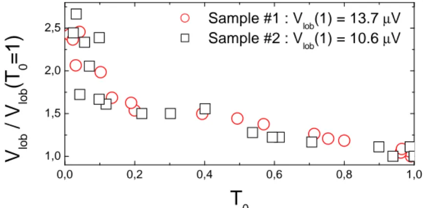
o`u T0 est la transmission du canal adjacent, ∆ν la mˆeme bande passante et Vϕun param`ete de d´ephasage. Nous avons repr´esent´e figure 2.9(b), le logarithme de la visibilit´e en fonction de V2 `a T0 fix´e `a 1/2, et figure 2.10 le logarithme de la visibilit´e en fonction de T0 pour

diff´erents V2. 0,0 0,2 0,4 0,6 0,8 1,0 0,0 0,1 0,2 0,3 0,4 0,5 V is ib ili ty T₀

Figure 2.10 – (couleur sur la figure)D´ependance de la visibilit´e en fonction de T0 pour

V2=0, 21, 31, 42, 53 et 63 µV de haut en bas. Les lignes en trait plein sont les fits aux

donn´ees exp´erimentales en utilisant l’´equation 2.3 avec Vϕ = 7.2µV et T =25mK.

L’excellent accord avec la formule 2.3 confirme notre approche (approximation Gaus-sienne du probl`eme). Cette exp´erience nous permet d’extraire Vϕ sur tout le plateau ν = 2. Puisque l’on connaˆıt V0, nous sommes capables d’extraire de Vϕ la bande passante, tous

4,0 4,5 5,0 0 10 20 30 40 50 V₀ 4 kBTϕ/e

Champ magnétique (Tesla)

V 0 µ V ) 0 2 4 6 8 V ϕ e t 4 k B T ϕ /e ( µ V ) Vϕ

Figure 2.11 – (couleur sur la figure) V0et Vϕ en fonction du champ magn´etique. La courbe en pointill´ee est le comportement g´en´eral de 4kBTϕ/e (´echelle `a droite) mesur´e sur le mˆeme ´echantillon.

les param`etres du probl`eme ´etant maintenant connus.

Revenons maintenant `a notre hypoth`ese premi`ere qui est que les fluctuations thermiques du canal adjacent sont responsables de la longueur de coh´erence finie. Si cette hypoth`ese est vraie on devrait obtenir d’apr`es 2.2 et 2.4 :

eVϕ= 4kBTϕ (2.4)

o`u Tϕa ´et´e mesur´ee dans la pr´ec´edente partie. Nous avons repr´esent´e figure 1.11 l’ensemble de nos r´esultats sur le plateau ν = 2. On v´erifie bien la relation 2.4 sur tout le plateau : notre hypoth`ese premi`ere est v´erifi´ee. La d´ependance de la longueur de coh´erence en fonction du champs magn´etique provient elle de la variation du param`etre de couplage V0 sur la

plateau. Cette d´eviation vient probablement d’une longueur de trajectoire ´electronique effective variant avec B.

2.6

”Voltage Probe”

Nous d´ecrivons dans cette partie une exp´erience du type ”which path”. Le d´etecteur est compos´e d’une petit contact ohmique flottant que l’on couple `a un MZI par l’interm´ediaire d’une grille lat´erale (voir figure 2.12).

Lorsque la grille lat´erale est ouverte tous les ´electrons du bras inf´erieur vont ˆetre ab-sorb´es par le contact ohmique flottant puis vont ˆetre r´e´emis avec une phase al´eatoire. On s’attend donc `a voir la visibilit´e diminuer avec la transmission TP de la grille lat´erale. On montre qu’elle s’´ecrit :

ν = ν0×

p

RP (2.5)

o`u RP=1-TP. Figure 2.13, nous avons repr´esent´e en point rouge la visibilit´e renormalis´ee en fonction de RP=1-TP, la courbe noire ´etant le fit associ´e `a la formule 2.5 : l’accord est parfait.

Figure 2.12 – Montage exp´erimental : le bras inf´erieur (b) du MZI peut ˆetre connect´e `a un contact ohmique flottant qui joue le rˆole de voltage probe. Les CPQ G1 et G2 sont les lames s´eparatrices qui s´eparent et recombinent les trajectoires ´electroniques. Le CPQ GP permet de contrˆoler la probabilit´e de transmission TP vers le contact de probe. G’1 et G’2 sont deux CPQ additionnels qui sont pinc´es pendant

l’exp´erience. -0.15 -0.14 -0.13 -0.12 -0.11 -0.10 -0.09 0.0 0.2 0.4 0.6 0.8 1.0 (a) Gate Voltage V GP (Volt) R_P=1-T_P Vis/Vis_Max Sqrt(R_P) 0.0 0.2 0.4 0.6 0.8 1.0 0.0 0.2 0.4 0.6 0.8 1.0 1.2 (b) Vis/Vis_Max Sqrt(R_P) V is ib ilit y / M a x . V is ib ilit y Reflection R_P=1-T_P

Figure 2.13 –(a) Visibilit´e renormalis´ee, RP et √

RP en fonction de VGP, la tension appliqu´ee sur GP.

(b) Visibilit´e renormalis´ee en fonction de RP. La courbe noire est la loi en √

RP pr´edite par la th´eorie.

Cette exp´erience nous a permis de suivre la variation en phase caus´ee par un ´etat localis´e prˆet du CPQ et `a le mod´eliser grˆace `a une approche du type matrice de scattering. Enfin des mesures de bruit r´ealis´ees avec la grille lat´erale ouverte nous ont permis de confirmer la relaxation en ´energie dans un contact ohmique flottant.

Introduction

Contents

3.1 Toward Bell’s inequality in mesoscopic physics . . . 20

3.1.1 Definition of the entanglement . . . 20

3.1.2 EPR Paradox and Bell’s inequality . . . 20

3.1.3 Violation of the Bell’s inequality . . . 22

3.2 Electronic entanglement in the two-particle interferometer . 22 3.3 From the simple Mach Zehnder Interferometer to the two-particle interferometer . . . 25

3.3.1 The two-particle Aharonov-Bohm effect . . . 25

3.3.2 Technical realization . . . 28

3.4 Conclusion . . . 28 The goal of this thesis was the observation of the Bell’s inequalities violation in a mesoscopic conductor. The violation of Bell’s inequality is the answer to an intense debate between Bohr and Einstein during the 20’s. Einstein had doubts about the probabilistic interpretation of the quantum physics defended by Bohr and the school of Copenhague. In 1935, Einstein published his famous article :”Can Quantum-Mechanical description of physical reality be considered complete ?” [27]. In this article Einstein et al. show that quantum physics predicts state of two particles, with strong correlations in position and velocity. In particularly this EPR state predicts that if we measure the position or the velocity of one of the particle, we can extract the position or the velocity of the other one. According to Einstein et al, since the two particles can be arbitrary far away from each other, the measurement of one particle can not modify the state of the other one. Einstein et al. have deduced that each particle owns the precise value of its position and velocity before the measurement. Since quantum physics can not give simultaneously the velocity and the position, quantum physics is not complete. Bohr immediately replied [54], explaining that such a state can not be described as two individual states : the entangled state was born. The entangled state constitutes a unique object whatever the distance between the two electrons.

In 1965, Bell [13] discovered that the ”EPR” state described by Einstein should lead to a contradiction with quantum mechanics. This article was all the more important that it opened new possibilities to give an experimental answer. If Bohr’s representation of quan-tum mechanics was the correct one, in certain conditions, Bell’s inequality (later defined) could be violated. A major experiment which has shown that indeed Bell’s inequality could be violated with an entangled state of photons has been realized by Aspect et al. in 1982 [9].

The initial objective of this thesis was to realize the electronic analog of the Aspect et al. experiment.

In a first part, I will define the entanglement, and I will show that for a certain tuning of the polarizers (optical device used in the Aspect et al. experiment), the Bell’s inequality can be violated. I will then introduce the violation of Bell’s inequality in mesoscopic physics and describe the type of geometry that would enable us to observe this effect.

3.1

Toward Bell’s inequality in mesoscopic physics

3.1.1

Definition of the entanglement

We call tensorial product of two spaces E1 and E2, the space E noted E1

N

E2generated

by the basis obtained ”juxtaposing” vectors of the two basis |Φ1

ni and|Φ2pi :

|Φn,pi = |Φ1ni O

|Φ2_pi

We consider now two vectors of E1 and E2 : |Φ1i and |Φ2i. Then :

|Φi = |Φ1i

O |Φ2i

is by definition a vector of E.

However the reciprocal is wrong : there exists some vectors that can not be factorized in E and written as a tensorial product |Φ1i

N

|Φ2i. Such a state |Φi is entangled.

3.1.2

EPR Paradox and Bell’s inequality

We start with the singlet state :

|Φi = √1

2(|+zi|−zi − |−zi|+zi)

This state is an entangled state. We now suppose that particles 1 and 2 are spatially separated. The particle 1 is sent to Bob, the particle 2 to Alice. If Bob makes a measurement of the polarization of the particle 1 along the axis z, he will be able to forecast the particle 2 state. For example, if he measures +1, he will deduce that particle 2 is in the state |−zi. There is a perfect correlation. It exists examples of perfect correlations in the classical world. We consider a black and a white ball. One of the ball is given to Bob. He observes

it, and notices that it is white : it deduces that Alice has the black one. But this example is based on a fundamental hypothesis : each ball owns the information ”I form a pair white ball-black ball”. Could we imagine the same hypothesis, but with an entangled system ? For example the pair |+zi|−zi would own the information ”I form the pair (|+zi, |−zi)”, information that each particle would conserve when they are spatially separated. It means here that the system owns some hidden variables.

More generally, if we note A(−→a ) (resp. B(−→b )), the measurement along −→a 1 _(resp. −→_{b ),}

the most general way to model this hidden variable is to write these measurements as A(λ, −→a )( B(λ,−→b )) where λ is the hidden variable. I now make the hypothesis that each hidden variable has a certain probability distribution P (λ) with :

Z

dλP (λ) = 1 and P (λ) ≥ 0 The values taken by A(λ, −→a ) and B(λ,−→b ) are :

A(λ, −→a ) ± 1 and B(λ,−→b ) ± 1 The average value of the resulting product is then written :

EQ(−→a , − → b ) = Z dλP (λ)A(λ, −→a )B(λ,−→b ) I now consider 4 vectors −→a ,−→a0_,−→_{b ,}−→_b0 _{and I introduce :}

s(λ) = A(λ, −→a )B(λ,−→b ) + A(λ,−→a0_)B(λ,−→_{b ) + A(λ,}→−_a0_)B(λ,−→_b0_{) − A(λ, −}→_{a )B(λ,}−→_b0₎

This can be written in a different way :

s(λ) = (A(λ, −→a ) + A(λ,−→a0_))B(λ,−→_{b ) − (A(λ, −}→_{a ) − A(λ,}−→_a0_))B(λ,−→_b0₎

since A(λ, −→a ) = ±1 and B(λ,−→b ) = ±1, we immediately deduce that s(λ)=±2 or s=0. Hence Bell’s inequality [13] :

|EQ(−→a , − → b ) + EQ( − → a0,−→b ) + EQ( − → a0,−→b0) − EQ(−→a , − → b0)| ≤ 2 (3.1)

The theory of the hidden variables leads thus to the Bell’s inequality 2.1. We are going to show that these inequality can be violated by the measurement of an entangled state, confirming Bohr’s interpretation of quantum physics.

3.1.3

Violation of the Bell’s inequality

− →

b ) as a function of −→a and−→b , the direction of the two polarizers. In the plane xOz, −→a is defined by the angle θ1 with the X axis :

|+−→_ai = cos(θ₁)|+i + sin(θ₁)|−i

|−−→_ai = − sin(θ₁)|+i + cos(θ₁)|−i

(we get similar results for −→b with the angle θ2). I now express |Φi in the eigenstates basis

|±−→_ai for the particle 1 and |±−→

bi for the particle 2, we get :

|Φi = √1

2(sin(θ2−θ1)|+a, +bi+cos(θ2−θ1)|+a, −bi−cos(θ2−θ1)|−a, +bi+sin(θ2−θ1)|−a, −bi) I deduce from this expression the probability to measure, for example, +1 for the particle 1 and +1 for the particle 2 (noted P (+a, +b)). EQ(−→a ,

− → b ) is given by : EQ(−→a , − → b ) = P (+a, +b) + P (−a, −b) − P (−a, +b) − P (+a, −b) This finally gives

EQ(−→a ,

− →

b ) = − cos(2(θ2− θ1)) (3.2)

We consider now the configuration of the figure 3.1. It is straightforward to show that : |EQ(−→a , − → b ) + EQ( − → a0_,−→_{b ) + E} Q( − → a0_,−→_b0_{) − E} Q(−→a , − → b0_{)| = | cos(6θ) − 3 cos(2θ)|} If we choose θ=π/8 then : | cos(6θ) − 3 cos(2θ)| = 2√2 > 2

For certain values of θ, Bell’s inequality are violated. The hidden variables theory combined with the principle of locality does not apply for entangled states. An entangled state can not be interpreted as two individual states. It is a unique state composed of two particles.

3.2

Electronic entanglement in the two-particle

inter-ferometer

In the previous part, we have used very general arguments to prove that for a certain geometric configuration of the polarizers, the measurement of an entangled state violates Bell’s inequality. In this part, I will detail how this experiment can be realized. I will show that for an ingenious mesoscopic conductors geometry [74][73], we can obtain the mesoscopic analogous of the optical experiment realized by Aspect et al. in the 80’s to violate Bell’s inequality. [9].

θ

θ

θ

Figure 3.1 – Geometric configuration to violate Bell’s inequality. Measurements are realized along a,b,a’,b’, the different directions of the polarizers. The angle between a and b, a’ and b, a’ and b’ is equal to θ. The angle between a and b’ is equal to 3θ. For θ = π/8 we obtain the maximally entangled state.

Entanglement in mesoscopic conductors

We are interested here in the system described figure 3.2. Electrons emitted by reservoirs 1 and 2 can be either transmitted to B or reflected to A. In the following, we will focus on electronic correlations between regions A and B.

1 3 2 4 A+ A- B-B+ B A S

Figure 3.2 –Schematic representation of the conductor. A region source (S) composed of the injection (reservoirs 1 and 2) and two beam splitters. Injected electrons are sent towards region A and B. Region A(resp. B) is composed of one beam splitter and two detectors : ohmic contacts A+ and A- (resp. B+ and B-).

Noise measurements and post-selection of an entangled state The injected state is :

|Ψi = a+ 1a+2|0i

where a+

i is the creation operator of a particle at the ithcontact. We introduce the operators

bAn and bBn that model electrons emitted by the contact n after the beam splitter from the region S and that propagate respectively toward regions A and B. We can relate these states to the injected states with the scattering matrix :

µ bA1 bB1 ¶ = µ r t0 t r0 ¶ µ a1 a3 ¶ and µ bA2 bB2 ¶ = µ r t0 t r0 ¶ µ a2 a4 ¶

The injected state thus becomes :

|Ψi = [r2_b+

A1b+A2+ t2b+B1b+B2+ rt(b+A1b+B2− b+A2b+B1)]|0i

The cross correlation noise measurement2 _{gives a no null result only for the two particles}

states, where one particle is in the region A and the other in B. Consequently, the noise measurement selects the state :

|Ψ0i = rt[|1iAi|2iB− |2iAi|1iB]

which is an entangled state. Since the scattering matrix is unitary, the beam splitter has a transmission coefficient toward the ohmic contact A+ : t=sin(θA) (B+ : t=sin(θB)), and a reflexion coefficient toward A- : r=cos(θA)(B- : r=cos(θB)). We obtain then :

µ |A+i |A−i ¶ = µ cos(θA) − sin(θA) sin(θA) cos(θA) ¶ µ |2Ai |1Ai ¶ and µ |B+i |B−i ¶ = µ cos(θB) − sin(θB) sin(θB) cos(θB) ¶ µ |2Bi |1Bi ¶

We introduce the quantity :

Pαβ = Sαβ ×

h −4e2_V

where Sαβ ∼ hδIαIβi is the cross correlated power noise spectrum, and α (resp. β) is A+ (resp. B+) or A- (resp. B-). We obtain then :

PA+B− = PA−B+ = 1 2[sin

2_(θ

A) sin2(θB)+cos2(θA) cos2(θB)+2 sin(θA) sin(θB) cos(θA) cos(θB) cos(φ0)]

and

PA+B+ = PA−B− = 1 2[cos

2_(θ

A) sin2(θB)+sin2(θA) cos2(θB)−2 sin(θA) sin(θB) cos(θA) cos(θB) cos(φ0)]

(3.3) 2. I will detail the cross correlation measurement in the Chapter 4. For the moment, we just want to determine the electronic correlation between region B and A without worrying about the actual way it can be done.

where φ0 is a phase term. We suppose first that φ0=0. The previous expressions now becomes : PA+B− = PA−B+ = 1 2cos 2_(θ

A− θB) and PA+B+ = PA−B− = 1 2sin

2_(θ

A− θB)

One can realize that the electronic and the optical problems are similar through the correlation function :

E(θA, θB) = PA+B−− PA−B+− PA+B++ PA−B−

E(θA, θB) = cos(2θA) cos(2θB) + sin(2θA) sin(2θB)

which has the same form as formula 2.1. We know that the Bell’s inequality is given by −2 ≤ SB ≤ 2 where :

SB= E(θA, θB) − E(θA0 , θB) + E(θA, θB0 ) + E(θ0A, θ0B) For θA=π/8 , θB=π/4, θA0 =3π/8, θB0 =π/2, we obtain SB = 2

√

2 and Bell’s inequality are maximally violated.

3.3

From the simple Mach Zehnder Interferometer to

the two-particle interferometer

In the previous part, I have described the general geometry of a mesoscopic conductor that would enable us to violate Bell’s inequality. Here, I present the double ”MZI”3_{, a}

feasible sample that fulfills all the conditions to violate Bell’s inequality. We will show that before tuning the beam splitters to obtain the maximal violation, we must check that noise measurements probe the entangled part of the state. In order to do that, we will vary the Aharonov-Bohm phase defined by the different electronic trajectories and will show that the entangled part of the state can be revealed by Aharonov-Bohm oscillations in the cross-correlated noise measurements.

A schematic representation of the sample [74] is represented figure 2.3.

3.3.1

The two-particle Aharonov-Bohm effect

Contrary to the simple electronic MZI [37], two incoherent electronic sources inject a current in the MZI. If we now compare this geometry to the one described in the previous part (figure 3.2), we notice that it is very similar. The region S is now composed of the ohmic contacts 2 and 3 that will inject electrons, with C and D the beam splitters that will partition electrons. The regions A and B are now composed of the ohmic contacts 5 and 8 (the detectors), with A and B the beams splitters. The noise measurements are realized between ohmic contacts 5 and 8. We are going to detail the state measured by

Figure 3.3 –Schematic representation of the double MZI proposed by Samuelsson et al. [74] . Electrons are injected from contacts 2 and 3. Cross correlation noise measurements are realized between contacts 5 and 8. Keeping in mind the notations of the figure 3.2, the source S is composed of ohmic contacts 2 and 3 and beam splitters C and D. Region A is composed of beam splitter A and ohmic contacts 5 and 6. Region B is composed of beam splitter A and ohmic contacts 7 and 8. φ is the phase accumulated along the trajectory of an edge. For example φ1is the accumulated phase along the outer edge between the beam

splitters C and A. Cross correlation noise measurement between contacts 5 and 8 is sensitive to the two electrons Aharonov-Bohm phase φ = φ1+ φ2− φ3− φ4

this cross correlation noise measurement and show that it depends on the ”two electrons Aharonov-Bohm” phase.

We introduce f (²) the Fermi distribution of reservoirs 2 and 3, and f0(²) the Fermi

distribution of the other reservoirs. We want to calculate the correlation current between contacts 5 and 8. The general expression of the noise between contacts α and β can be written as : Sαβ = −2e2 h Σγδ Z dE(s+ αγsαδs+_βδsβγ)(fγ− f0)(fδ− f0) S58= −2e2 h Z dE|s∗ 52s82+ s∗53s83|2(f − f0)2 (3.4)

where sαβ is the scattering amplitude between contacts α and β. When the gates trans-missions are equal to 1/2 :

S58=

−e2

4h |eV |[1 + cos(φ1 + φ2− φ3− φ4)]

where φ1 is the phase accumulated between QPCs C and A, φ2 between QPCs D and B,

φ3 between QPCs C and B, φ4 between QPCs D and A (see figure 2.3). We suppose now

that we can add a magnetic flux through the sample. Due to the chirality of the electronic trajectories, we obtain a positive contribution of the magnetic flux for the phases φ1 and

magnetic flux is thus equal to φ1 + φ2− φ3− φ4 =

H −→

dl .−→A where −→A is the potential vec-tor. Varying the magnetic flux through the double MZI, we should observe two electrons Aharonov-Bohm oscillations. 3 5 4 φ 2 φ A C D B 2 φ3 1 φ 8 a) b)

Figure 3.4 –(a) Schematic representation of the first version of our double MZI . There is no side gate to tune each simple MZI separately. Electrons are collected via small inner ohmic contacts in yellow on the figure.(b) Zoom of the central part of the double MZI with four gates, and two ohmic contacts connected to the ground. The advantages of this sample was the very short length of the trajectory. The disadvantage was the impossibility to tune the interferometer using conductance measurements.

Once two-electron Aharonov-Bohm oscillations measured, how can we violate Bell’s inequality ? Comparing formula 3.4 to 3.2 obtained in the previous part, we then obtain :

P58∼ 1

2[sin

2_(θ

A) sin2(θB) + cos2(θA) cos2(θB) + 2 sin(θA) sin(θB) cos(θA) cos(θB) cos(φ0)]

once P58 measured, we have to set φ0=0, to reproduce the measurement with P67, P68 and P57 tuning θA=π/8 , θB=π/4, θ0A=3π/8 and θ0B=π/2.

3.3.2

Technical realization

Figure 3.5 –Schematic representation of the second version of our double MZI. Electrons are injected from contacts 2 and 3. Cross correlation noise measurements are realized between contacts 5 and 8. Keeping the notations of the figure 3.2, the source S is composed of ohmic contacts 2 and 3 and beam splitters C and D. Region A is composed of beam splitter A and ohmic contact 5. Region B is composed of beam splitter A and ohmic contact 8. φ is the phase accumulated along the trajectory of an edge. For example

φ1 is the phase accumulated along the outer edge between the contacts C and A. Cross correlation noise

measurement between contacts 5 and 8 should be sensitive to the two electrons Aharonov-Bohm phase

φ = φ1+ φ2− φ3− φ4. A side gate (SG) enables us to separate the upper MZI from the lower one. We

should first tune separately each simple MZI to obtain the highest visibility and then open the side gate and realize noise measurements, as it has been done recently by the Weizmann group [60].

We started the experiment with a sample which was exactly the one proposed by Samuelsson et al [74]. These samples (see figure 3.4) had the advantage to be very compact hence leading to very short electronic trajectories. However these samples suffered from a strong disadvantage : it was impossible to tune the magnetic field and/or the gate voltage to obtain the highest visibility using conductance measurements. We have chosen then a configuration pioneered by the Weizmann group [60] (see figure 3.5). The trick is to separate two simple MZI by a gate : when the gate is closed, we tune separately the two MZI using conductance measurements, to obtain the highest visibility on each. When the gate is opened we get the double MZI configuration [60] and can perform noise measurements.

3.4

Conclusion

This chapter was a general introduction to this thesis. We have shown that it is theoreti-cally possible to violate Bell’s inequality with a mesoscopic conductor. We have described the geometry to achieve this experiment. Starting with two simple MZI tuned in order to measure the highest visibility, we open the central gate and obtain the Double MZI

configuration. We will then probe the entangled part of the state via electronic shot noise measurements These measurements will be realized at finite bias voltage and finite tem-perature. Consequently before measuring the noise, we need to study the visibility in a simple MZI as a function of the sample size, magnetic field and applied bias.

1. We first have to extract a coherence length, since when we will open the central gate, the surface of the interferometer will be doubled : we have to ensure that the two electrons state remains coherent on the whole surface.

2. We have to find a magnetic field where this coherence length is the longest. This study of the coherence length will give us the temperature dependence of the visibility : we will then be able to know if the electronic temperature of our fridge (20mK) will be low enough to measure the two electrons Aharonov-Bohm effect.

3. Finally since the noise measurements are realized at finite bias voltage, we must understand the voltage bias dependence of the visibility. Recent experiments have shown that the voltage bias dependence of the visibility was not monotonous [57] : such results must be explained before performing noise measurements.

After all these preliminary studies, we will be able to answer this question : do we have the noise sensitivity to violate Bell’s inequality with our experimental set up ?

Chapitre 4

The electronic MZI

Contents

4.1 Introduction . . . 31 4.2 From optics to mesoscopic physics : description of the optical

MZI . . . 31 4.3 An electronic beam : the edge state of the Integer Quantum

Hall regime . . . 33 4.3.1 The classical Hall effect . . . 33 4.3.2 The quantum Hall effect . . . 34 4.3.3 Electrons without spin . . . 35 4.3.4 Electrons with spin . . . 36 4.3.5 Hall resistance and Shubnikov-de-Haas oscillations . . . 36 4.3.6 Edge states . . . 37 4.4 Electronic Beam Splitter : the Quantum Point Contact . . . 39 4.4.1 The Quantum Point contact . . . 40 4.5 The electronic Mach Zehnder Interferometer . . . 41 4.5.1 Description . . . 41 4.5.2 Fabrication process . . . 42 4.5.3 The two dimensional electron gas . . . 42 4.5.4 Aharonov Bohm oscillations . . . 43 4.6 Experimental technics . . . 44 4.6.1 Conductance measurements . . . 44 4.6.2 Noise measurements . . . 45 4.6.3 Measuring the visibility in the MZI . . . 47 4.7 Conclusion . . . 50

4.1

Introduction

This part is an introduction to the electronic MZI and the experimental set up. We will first recall the historical experiment of the MZI realized in optics and we will explain its general principle. In optics, interferometers are composed of beams splitters, mirrors and source of photons. To realize interference experiments in mesoscopic physics which are somehow a copy of the one realized in optics, we must find an experimental set up which produces beam-like electronic motion, beam splitters, mirrors. We will show that the edge states in the quantum Hall regime are 1D wires whose position can be easily controlled. In a second step, we will take up the question of the beam splitters : we will show that the quantum point contacts (QPC) are good candidates to mimic beam splitters. Then, we will describe the geometry of the electronic MZI and explain how the conductance and noise measurements are performed.

In a last part, we will detail the method that we have followed to obtain the highest visibility on samples with a stable phase (several hours) and also with samples presenting phase fluctuations.

4.2

From optics to mesoscopic physics : description of

the optical MZI

Beam Splitter 1 Beam Splitter 2 Mirror Mirror Detector Sample

Figure 4.1 – Schematic view of the optical MZI. A collimated beam is split by a first half-silvered mirror (represented in grey). The two resulting beams (the ”sample beam” and the ”reference beam”) are each reflected by a mirror (in black on the figure). The two beams are recombined on a second half-silvered mirror and then enter in the detector.

The Mach Zenhder interferometer1 _{is a device which has been used for the first time}

to determine the phase shift caused by a small object placed in the path of one of two collimated beams issued from a coherent light source.

A collimated beam is split by a half-silvered mirror (a beam splitter). The two resulting beams (the ”sample beam” and the ”reference beam”) are each reflected by a mirror. The two separated beams are then recombined on a second half-silvered mirror and then enter in the detector.

Because the coherence length of photons is larger than the size of the interferometer , the transmission amplitude t through the MZI is the sum of the two complex transmission amplitudes corresponding to upper path and down path of the interferometer. For trans-mission and reflection amplitudes ti and ri for the ith beam splitter (with |ri|2+|ti|2=1 (i=1,2)), the transmission amplitude t through the MZ is given by :

t = t1ei(δke+kLu)r2 − r1eikLdt2.

where k is the wave vector of the monochromatic light, δk the wave vector variation due to the inserted object and e the thickness of this object2_{. It leads to the transmission}

probability :

T = T1R2+ R1T2+

p

T1T2R1R2sin(ϕ)

where ϕ(k) = k(Lu− Ld) + δke and Ti=|ti|2 = 1 − Ri.

To reveal oscillations, one has to vary the length difference between the two trajectories by moving one mirror, or to introduce a phase shift by adding a sample along one of the path.

One of the major difficulties when making an optical interferometer was to obtain a focussed light beam and a monochromatic one, such that the coherence length of the source (inversely proportional to its spectral width) is longer than the interferometer. For several decades, the LASER has been very useful as it provides directly a focussed monochromatic light.

Here, one wants to make interferences with electrons : the electronic wave function replaces the electromagnetic one. If interferences with electrons have already been realized in mesoscopic conductors [19][77], it is impossible to impose strictly two trajectories for electrons without chirality3_{(at least in conductors). This problem is circumvented here by}

breaking the time reversibility of trajectories with a magnetic field. We will show that when submitted to a perpendicular magnetic field, the electronic transport in 2D high mobility electron gas is chiral and occurs along edge states which are 1D conductors. Consequently, we will be able to control the trajectories of electrons just by designing the edge of the sample. Another major difficulty when making an optical interferometer is the tuning of beam splitters. The collimation of the transmitted and reflected beams must be very precise, and the transmission of each beam splitter has to be set to 1/2 in order to obtain

1. Named after physicists Ludwig Mach and Ludwig Zehnder (1891) [47][89].

2. The sign minus in the reflection is a consequence of the unitary of the scattering matrix. 3. Motion in one direction, like a photon beam.

the highest visibility. In mesoscopic physics, we will show that QPCs enable us a very accurate tuning of the electronic beams transmissions. Last, ohmic contacts will serve as detectors of electrons, and detection will be realized via voltage measurement between two ohmic contacts.

4.3

An electronic beam : the edge state of the Integer

Quantum Hall regime

Before describing the edge states properties, I will give a brief introduction of the quantum Hall effect. Then, I will describe the electronic transport in the quantum Hall regime and show that the transport occurs in 1D wires along the sample edges : the edge states.

4.3.1

The classical Hall effect

Classical Dynamics of electrons submitted to a magnetic field

We consider a 2D gas of electrons submitted to a perpendicular magnetic field −→B . We introduce the complex notation z=x+iy to study the position of electrons. The dynamic of electrons under the Lorentz force is :

m¨x = −eB ˙y and m¨y = eB ˙x

or ¨z = iωc˙z with ωc=eB/m∗, where¨denotes the second time derivative, and m∗the effective mass. The solution of this simple equation is given by :

z = C − iv0 ωc

eiωct

For non zero values of v0, the trajectory of the particle describes a cyclotron orbit with a

frequency ωc. The center of this orbit C is fixed.

Transport

In the classical Hall regime, the conductivity tensor ˆΣ (defined by −→j = ˆΣ−→E ) is equal to [7][38] : ˆ Σ = Σ 1 + ω2 cτ2 µ 1 −ωcτ ωcτ 1 ¶

where Σ is the conductivity at zero magnetic field, Σ=nse2τ /m∗, τ being the Drude collision time. We deduce from that expression the resistivity tensor :

ˆ ρ = ( ˆΣ)−1 _{= ρ} µ 1 ωcτ −ωcτ 1 ¶

with ρ=Σ−1 _{the resistivity at zero magnetic field. The longitudinal resistivity is given by} the diagonal elements of the tensor, and the Hall resistance (or transverse resistance) by its non-diagonal elements. We note that in the classical regime, the longitudinal resistance is not affected by the magnetic field and the Hall resistance is given by :

ρxy = ρωcτ = 1 nse

B

The classical Hall resistance varies linearly with the magnetic field and offers the possibility to measure the electronic density. This classical description of the Hall effect is adapted for ωcτ ¿ 1. The transition with the quantum Hall effect occurs when the collision time τ of the electrons is larger than the inverse of the cyclotron frequency and the temperature of the system T ¿ ~ωc.

4.3.2

The quantum Hall effect

The discovery of the Quantum Hall effect in 1980 by Von Klitzing [39] has been an im-portant step in the comprehension of the electronic transport in 2D systems. Von Klitzing et al. have characterized the variations of the longitudinal resistivity ρxx, and of the trans-verse resistivity ρxy of a two-dimensional gas with the applied magnetic field. If in average

ρxy followed a linear slope with B as predicted by the classical approach, Von Klitzing has observed some plateaus at 1.5K. These plateaus in the curves ρxy have the remarkable property to appear at values equal to h

e2 × 1_ν where ν is an integer : this quantification is

the mark of a quantum phenomenon (figure 4.2).

Figure 4.2 –Hall and longitudinal resistance as a function of the magnetic perpendicular field. We note the integer Hall plateaus, and the Shubnikov-de-Haas oscillations between two plateaus. The longitudinal resistance is null on the Hall plateaus.

For each plateau, Von Klitzing noticed that ρxx vanishes : the electronic transport is no

longer dissipative. He also observed some peaks of ρxx while ρxy was evolving continuously

between two plateaus. These oscillations are the expression of a well known phenomena for electrons submitted to a uniform magnetic field : the Shubnikov-de-Haas oscillations. [28].

4.3.3

Electrons without spin

To explain the origin of these plateaus, we first consider the simple case of an electron moving in a 2D system, submitted to a perpendicular magnetic field. Here, we will neglect electronic interactions. The Hamiltonian of the system is given by :

H0 = 1 2m∗(− →_{p − e}−→_{A )}2 ₌ Π2 2m∗ = 1 2m∗(Π 2 x+ Π2y)

with m∗ _{the electron effective mass, e=−|e| its charge, −}→_{p its moment, and}−→_{A the potential} vector. In the cylindric gauge,−→A = 1

2

− →

B ∧ −→r with−→B the magnetic field, we can show that the hamiltonian is quadratic in position and in moment. The problem is thus analog to an harmonic oscillator in two dimensions, Πx and Πy being conjugate :

[Πx, Πy] = −i~2 l2 m where lm= p

~/eB is the cyclotron length. We introduce the operators a and a† _defined by :

a = lm

~√2(Πx− iΠy) and a

†₌ lm

~√2(Πx+ iΠy) leading to [a, a †_{] = 1}

The Hamiltonian H0 becomes :

H0 = ~ωc(1 2+ a

†_a)

The energy spectrum of this Hamiltonian is given by εn = ~ωc(n + 1₂). These discrete energy levels are called Landau levels. The charged particles can only occupy orbits with discrete energy values : between two Landau levels, there are no available states. As the density of state falls to zero between 2 Landau levels, it would mean that the system should be a perfect insulator. In fact, the explanation of the Hall plateau is a little bit more sophisticated. As an example the sample edges and the disorder play a crucial role. Since H0 does not depend of the position of the center of the cyclotron orbit, energy levels

must be degenerated. The quantum operator that describes the position of the center of the cyclotron orbit is defined by :

C = z + i Π m∗_ω

c

which leads to [Cx, Cy] = ilm2

where z=x+iy stands for the position of the cyclotron orbit. 2πl2

m represents the area of one flux quantum φ0=h/eB. We now introduce operators b and b† :

b = 1

lm

√

2(Cx+ iCy) and [b, b †_{] = 1}