Detection of localized structures from multispacecraft data: Adaptive correlation function

HAL Id: hal-00408538

https://hal.archives-ouvertes.fr/hal-00408538

Submitted on 13 Mar 2021

HAL is a multi-disciplinary open access

archive for the deposit and dissemination of

sci-entific research documents, whether they are

pub-lished or not. The documents may come from

teaching and research institutions in France or

abroad, or from public or private research centers.

L’archive ouverte pluridisciplinaire HAL, est

destinée au dépôt et à la diffusion de documents

scientifiques de niveau recherche, publiés ou non,

émanant des établissements d’enseignement et de

recherche français ou étrangers, des laboratoires

publics ou privés.

Detection of localized structures from multispacecraft

data: Adaptive correlation function

L. Rezeau, G. Belmont, F. Reberac

To cite this version:

L. Rezeau, G. Belmont, F. Reberac. Detection of localized structures from multispacecraft data:

Adaptive correlation function. Journal of Geophysical Research, American Geophysical Union, 1998,

103, pp.2319-2326. �10.1029/97JA02666�. �hal-00408538�

JOURNAL OF GEOPHYSICAL RESEARCH, VOL. 103, NO. A2, PAGES 2319-2325, FEBRUARY 1, 1998

Detection of localized structures from multispacecraft data:

Adaptive correlation function

L. Rezeau, G. Belmont, and F. Reberac

Centre d'rtude des Evironnements Terrestre et Planrtaires, Universit6 de Versailles Saint-Quentin, V61izy, France

Abstract. When several

spacecraft

pass

at different distances

from a localized structure

like a field-

aligned

current

tube, the corresponding

magnetic

signatures

recorded

on each spacecraft

generally

show different timescales,

due to the different "viewpoints"

of the spacecraft.

For this reason,

it is

impossible

to identify the presence

of a unique structure

from these

signatures

by using the

classical

correlation

functions.

In this paper, we present

an "adaptive

correlation

function"

which is

a new analysis

tool allowing to look for such "correlations"

whatever

the dilation factor is between

two signals.

1. Introduction

In space plasmas, many objects of physical significance are localized in space, and their signatures are thus concentrated in time along the spacecraft trajectories. A

paradigm for such structures can be a static cylindrical field-

aligned current tube (FAC), resulting for instance from the filamentation of a current sheet. As the magnetic field created by a FAC is easy to calculate, it is possible to search the magnetic field data for resembling signatures [Robert et al.,

1984]; when such a signature is visually picked out, one can

determine the few parameters of the model by a numerical fit

(intensity of the current, distance from the spacecraft, and relative velocity). The short large amplitude magnetic structures (SLAMS), [Schwartz et al., 1992; Dudok de Wit and Krasnosel'skikh, 1995], which are observed upstream of

quasi-parallel shocks, are other structures (more complex but

still quasi-static) which can also be investigated in the same spirit.

When trying to extend the above method, one comes up against two limitations:

1. There is no uniqueness of the interpretation and most

generally no means for testing the validity of the model chosen for the observed signature. This first limitation is met in particular when the structure can be supposed to have a temporal evolution, as in the case of kinetic Alfven waves

[Chmyrev et al., 1988, Rezeau et al., 1993]: the

eigenfrequency then mixes with the Doppler frequency because of the apparent motion and the number of independent data necessary to disentangle time and space variations becomes much larger. It is quite possible that the same event identified as a FAC from the only magnetic field data at one spacecraft can be interpreted as well by a kinetic Alfven wave or by a combination of both (Alfven solitons). The only way to go beyond this limitation is to increase the

amount of data comparable with the model, so decreasing the

probability of multiple interpretations (in particular by the use of multispacecraft experiments).

Copyright 1998 by the American Geophysical Union. Paper number 97JA02666.

0148-0227/98/97JA-02666509.00

2. Even when localized signatures can be picked out visually in different signals, the question of whether these signatures are due to the same structure or have independent

causes cannot always be answered. In particular, the use of

correlation methods often fails when the signals are recorded

on different spacecraft. We will try to bring a solution to this

specific problem.

In order to restrict the possibilities of multiple interpretations, especially to disentangle space and time variations, the best way thus appears to be the use of

simultaneous data from several close spacecraft. This was one

of the motivations of multispacecraft missions such as ISEE

or Interball, and a lot of work has been done in this field in

the frame of the CLUSTER project preparation. The data processing methods now exist to get decisive physical

information out of the data when the measurements are made

inside a structure with a typical scale larger than the

interspacecraft distance, e.g., intensity of the local current

imbedded [Robert and R oux, 1990] or a study of waves through an estimation of thewavenumber spectrum for each frequency [Pincon and Lefeuvre, 1991] or through recognition of the wave mode [Motschmann and Glassmeier, 1995].

Nevertheless, as discussed by Rezeau et al. [1990], when the

spacecraft remain outside of a small current structure (compared to interspacecraft distance), the magnetic signatures recorded on each of them present different characteristic scales and amplitudes because of the different viewpoints of the different spacecraft: as the magnetic field

created by a current tube decreases with the distance to the

source, a spacecraft passing by the tube at a short distance records a narrow and intense signature, whereas a spacecraft passing at a large distance records a wide signature with a weak intensity. Then, all classical tools such as correlation functions or spectral analysis fail in diagnosing the structure even in this simple case of a pure FAC. The same conclusions

came out of an experimental study performed on ISEE 1 and 2

data [Rezeau et al., 1993] in a case where the observations are

very similar on both spacecraft and where many indications show that it is most probable that the same localized structure

is observed on both spacecraft: the spectral analysis indicates

a frequency shift of the peaks in the power spectra, and

consequently the cross-correlation functions between the two

2320 REZEAU ET AL.: ADAPTIVE CORRELATION FUNCTION

spacecraft signals have a very weak maximum. These studies

indicate that a satisfactory method should take into account this viewpoint effect which is different from one spacecraft to another. A new method has been developed, the adaptive correlation function, which is derived from the wavelet analysis of signals. The application of the method to ISEE data will show its efficiency. It must be noticed that the present work is limited to the identification of signatures of different scales but similar shapes. It could be extended in the future to signals that are physically related (due for instance to the derivatives contained in the Maxwell equations) without having the same shape.

The method is obviously not limited to the particular case

presented here of magnetic signatures, it should be useful in

any case when geometrical effects around a localized structure

are to be taken into account whatever the data. It could be

applied to the density or the velocity of the plasma. 2. Data and Method Baseline

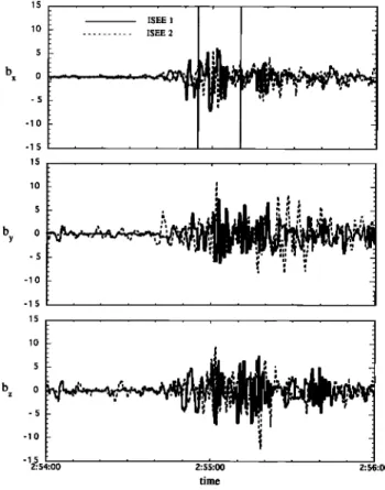
The method will be described and applied to the same case as in the work of Rezeau et al. [1993]: a localized structure observed on magnetic fluctuations at the inner edge of the boundary layer, with a small delay between ISEE 1 and 2 (November 8, 1977, around 0255 UT). The data are the flux gate magnetometers data since the ISEE search-coil magnetometers frequency range does not allow the exploration of the ultra-low-frequency range (Figure 1).

Nevertheless,

a filtering

by subtraction

of a running

average

over 5 s has been applied to eliminate the large-scale

lO 5 b x o -lO -15 15 b 0 y -5 -10 -15

. ! 1%,•

II

II

i

Figure 1. Waveforms of the magnetic fluctuations

(nanoteslas) observed on ISEE 1 and 2, projected in the

magnetopause LMN frame.

variations of the field (which are similar on both spacecraft) and keep only the fluctuations (which could be different from one spacecraft to another). It makes the inspection of the fluctuations clearer, but it is not a necessary step; the method presented here could be applied on the nonfiltered data. The results obtained by Rezeau et al. [1993] show that the signals

on the two spacecraft are correlated (the maximum correlation

(0.6) is obtained for a delay equal to 2 s) but that there is a

discrepancy in the spectral features (the relative maximum of

the spectrum is at 0.6 Hz on ISEE 1 and 0.8 Hz on ISEE 2. Nevertheless, they are likely to be interpreted as two

signatures of a unique structure convected by the plasma flow.

The baseline of the adaptive correlation method is derived from the wavelet analysis, but it is not a new wavelet theory.

The main properties of the wavelet transform with respect to

the Fourier transform are the localisation of the analyzing function and the self-similarity. For instance, if we consider the Morlet wavelet analysis, it can be compared to the Fourier transform: the elementary analyzing function is a limited complex exponential instead of an unlimited complex

exponential [Grossmann et al., 1989; Lagoutte et al., 1992].

The limitation is obtained by multiplication by a gaussian function with a width equal to a few periods of the complex exponential whatever the frequency. For this reason, the wavelet analysis is better adapted to the study of transient or localized signals than the Fourier transform. When applied to the signals of Figure 1, a wavelet analysis will emphasize

the fluctuations around 0255:00 UT on both spacecraft; it will

show that the maxima are observed at times slightly different

with close timescales, but it will obviously not give any indication on their possible correlation. The adaptive correlation function is a correlation function modified to get a localized diagnosis in the same spirit as in wavelet theory. The method consists in the following steps: (1) pick out an event on one component recorded on one of the two

spacecraft (the corresponding data will be referred hereafter as

RS, reference signal), (2) extract the desired pattem (supposed to be related to an interesting physical phenomenon) from it by filtering to prepare a reference function (similar to mother wavelet in wavelet analysis), (3) dilate (or contract) and delay this function to analyse another signal (AS, analyzed signal), generally the same component recorded on the other spacecraft. The result of this analysis will be a three- dimensional diagram similar to the wavelet scalogram, with

time as horizontal axis and scale (i.e. dilation relative to the

RS scale)as vertical axis. It will evidence the times when

signals are correlated on the two spacecraft, and the relative

time scales of the two viewpoints. From this comes the name adaptive correlation given to the method.

3. Description of the Method

The first step is the choice of the RS from the visual identification of an "event." On the example of Figure 1, we select about 10 s around 0255:00 UT on the B x component

recorded on ISEE 2. The simplest way would then consist in

taking the signal itself as analyzing wavelet. The tests that have been performed show that, because of the superimposed noise, this method is not efficient (see section 4). The signal

has to be filtered before use, and the method chosen here is

the singular-spectrum analysis (SSA). As it will be shown

below, this method is very efficient to separate trend and

oscillatory

part of the signal,

without

fixing an arbitrary

low-

RE7F•AU

ET AL.:

ADAPTIVE

CORRELATION

FUNCTION

frequency cutoff. The software used is the one developed by

Dettinger et al. [1995] and described by Vautard et al. [1992].

This spectral analysis method is dedicated to short and noisy

signals. It is a decomposition of the signal on

eigenelements, and the specificity of the method is that these

eigenelements are data-adaptive; they are not given as inputs

like in Fourier transform. After this decomposition on the

eigenvectors, called principal components, the signal can be

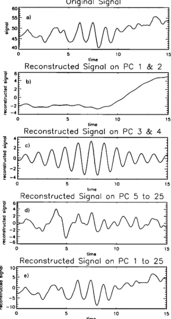
filtered by reconstructing it from only a subset of the principal components. On Figure 2, the method has been applied on the RS over 16 s beginning at 0254:54 UT. The original signal is displayed in Figure 2a (the running average filtering has not been applied before SSA analysis to bring out the capability of the method); in Figures 2b-2c, the

reconstruction of the signal on different subsets of principal

components are shown. It evidences the efficiency of the method for separating the trend (low-frequency part of the signal), the oscillatory part and the high-frequency noise of

the signal. The number of principal components on which the

signal is split is a free parameter called the "embedding dimension"; it has been chosen here equal to one fourth of the total number of points of the time series. From the previous study [Rezeau et al., 1993], it seems that a localized structure is the cause for the oscillatory part of the signal around 0255 UT; we therefore choose the reconstruction on principal

components number 3 and 4 as analyzing function.

Once the reference function g is chosen, we use it to analyse a signal. For that purpose, we compute a scalogram, which is similar to a spectrogram but with a computation window increasing with scale in the same way as in wavelet analysis [Grossmann et al., 1989]. A family of daughter functions is generated by dilation and translation in time:

ga,b(t) (see Appendix for details). Both dilation and

scale decreases. For each value of a and b the correlation

coefficient

Cg,s(a,b)

is computed

and displayed

with a color

code on the scalogram.

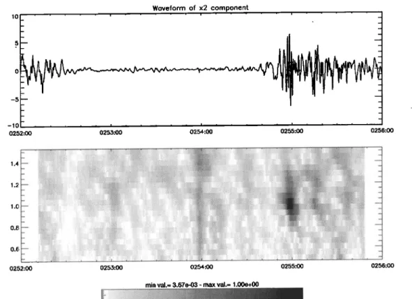
The result is shown in Figure 3b. The horizontal axis is time, the vertical axis is scale (or "dilation": scale is 1 for the mother wavelet); the maximum scale is at the top of the diagram. The pixel width increases with scale, it is equal to 5% of the wavelet width. As a test, the program has been first applied to RS. As expected the maximum of the correlation function is obtained for a dilation equal to 1, at time t = 0255:01.6, time of the maximum of the signal.

More interesting is the result shown on Plate lb, where AS

is the B x component recorded on ISEE 1 (Plate la). Four main

maxima are seen with the characteristics shown in Table 1 (in

order of decreasing value of the maximum). The first point is

that none of these maxima correspond to a dilation equal to 1,

which means that the viewpoints of the two spacecraft are actually different. One of the maxima (3) evidences the same delay as the classical correlation computation (delay equal to 2 s, [Rezeau et al., 1993]), it is obtained for a dilation equal to 1.3. This result is consistent with the spectral analysis performed in the same study, which gave frequency maxima at

0.6 and 0.8 Hz, which means a scale factor of

0.8/0.6= 1.33 between the observations on the two

spacecraft.

Plate lc shows the final form proposed for the visualisation of the result. This last change aims to answer

Original Signal

Reconstructed Signal on PC 1 & 2

6

0 5 10 15

time

Reconstructed Signol on PC 5 & 4

'• -2 • --4 0 5 10 15 time

Reconstructed Si9nol on PC 5 to 25

Reconstructed Signol on PC 1 to 25

Figure 2. Singular-spectrum analysis (SSA) filtering. (a) Waveform of the reference signal (B x component measured by ISEE 2, total magnetic field). The horizontal axis is delay in

seconds from the beginning of the selection (0254:54). The

time period presented corresponds to the vertical lines on Figure 1 (top). (b)-(e)Reconstruction of the signal using different subsets of principal components determined by SSA. Figure 2e shows the reconstruction on the 25 first

components: it is identical to the original signal (Figure 2a),

except for the average which is lost by SSA.

the following difficulty: as the correlation coefficient has been calculated to be independent upon the power in the correlated signals, large values may correspond to very weak components in the analyzed signal. This property obviously increases the probability of spurious correlations between the analyzing wavelet and many small components of the signal which are not physically significant. To avoid cluttering the display with such parasitic correlations, Plate lb has been modified in the following way: instead of plotting the correlation coefficient, we only use it as a criterion to select the nonnormalized correlation function which is proportional

2322 REZEAU ET AL.: ADAPTIVE CORRELATION FUNC•ON

a)

b)

min vaJ.= 5.53e-03 - max val.= 6.73e-01

c)

rain val.= 1.30e-03 - max vaL= 6.81e-02

0256:00

Plate 1. (a and b): Result

of the analysis when applied

to the same component

on the other spacecraft

(ISEE 1). The dilation scale

goes from 1 to 2. Four maxima

are observed,

they are labeled

from 1 to 4 with

decreasing

correlation.

(c) The normalized

correlation

is used

as a filter for the plot of the nonnormalised

correlation.

The colored

region

is the region where

the correlation

is higher than 0.4; inside this region the

to the intensity of the correlated signals. In the regions of the plane where the correlation coefficient is lower than a given threshold (chosen equal to 0.4 here), the color plot of the nonnormalized correlation function is masked. When it is

plotted, this nonnormalized correlation is directly

wavelet is normalized. The interpretation of the four maxima

observed on Plate 1 b is modified by this analysis, two of them (2 and 3) appear more interesting since they are both correlated and intense events (they are identified by * in Table 1 and their intensities are respectively 0.0679 and 0.0681). Therefore, in addition to the maximum at 1.3 dilation (3), the maximum corresponding to 1.6 dilation (2) appears

significant although it was not evidenced by the classical correlation analysis, the other one was the already identified one. The result of this analysis is that the signature observed on ISEE 2 appears to be correlated with two signatures on ISEE 1. This is still to be physically interpreted, but this example shows that the improvement of the correlation method was necessary.

4. Discussion and Conclusion

We have shown in this paper that the classical correlation methods used to detect in different signals similar wave forms

with equal

timescales

cannot

be used

without

change

to detect

REZEAU ET AL.: ADAFI• CORRELATION FUNCTION 2323 Waveform of x2 component _ _ 0 i I i i i i i 0252:00 0253:00 0254:00 0255:00 0256:00 -113

0'8

I

min val.= 3.67e-03 - max val.= 1.00e+00

Figure 3. Result

of the analysis

when

applied

to the reference

signal

(Figure

3b). The horizontal

axis is

time. The dilation is shown on the vertical axis, with a linear scale from 0.5 to 1.5. As expected when

analyzing

the reference

signal,

the maximum

is obtained

for a dilation

equal

to 1.

the signatures

of a spatial structure

from different

spacecraft,

viewpoints

of the spacecraft.

The method

proposed

makes

use

analysis

(to isolate

the signature

to be correlated)

followed

by

with an adequate

visualisation,

the method

has been shown

on

an example

to be powerful

and to allow the detection

of a

from 1.

An element of the method has still to be discussed: why

not to use the signal itself as an analyzing

wavelet?

It would

analysis.

The reason

is that like the analyzed

signal, the

original signal contains

many components,

including

high-

frequency noise (and eventually trend). For the same reason as

in the preceding

section, keeping all of these components

Table 1. Characteristics of the Maxima Observed in Plate lb (labeled from 1 to 4 With Decreasing Value of the Maximum)

Maxima Time Delay (s) Dilation Correlation

1 0255:17.6 16 1.32 0.68 2* 0254:58.8 -2.8 1.58 0.57 3* 0255:03.9 2.3 1.32 0.49 4 0255:19.0 17.4 1.58 0.48 * events for which the nonnormalized correlation is the most intense (see Plate lc)

greatly

increases

the number

of spurious

correlations

between

figure

cluttered

by a lot of nonsignificant

high values

of the

wavelet translation step to the next because

of the high-

frequency noise; the method would then demand a step as

small as possible

(sample

time) because

of these

artificial

fine structures.

With the filtered signal, on the contrary, a step

corresponding

to a fraction

of the length

of the analyzing

function is sufficient (4%). For a dilation equal to 1, in our

case,

this means

steps

of 12 sample

times and the obvious

consequence

is a significant

save in computation

time. It

must

be noted

that larger

pixels

still give the same

result,

and

From the results obtained for the given example, it appears

that the interpretation

is still not straightforward

since

the

selected

signature

on ISEE 2 is correlated

with two signatures

on ISEE 1. Of course, we cannot grant that when two

signatures

are correlated,

they do correspond

to the same

event.

It is possible

that one signature

corresponds

to the

same event but that the other one is the signature of an event

that is similar

without

being

the same.

It is also possible

that

the second

event is seen by only one spacecraft

and not by

the other.

This could lead to conclude

that the mother

function

is so generic

that

it correlates

with any wave

packet:

this is

not true

since

only two events

are selected

by the method,

while a visual inspection

of the signals

after 0255:00 UF

evidences the existence of other wave packets that are not correlated with the mother function. However, the results

2324 REZEAU ET AL.: ADAPTIVE CORRELATION FUNCTION

obtained confirm that the signal processing tool that we propose is able not only to quantify correlations which are apparent by visual inspection but also to detect possible correlations which are less obvious at first glance.

The adaptive correlation function, in its present form, enables one to detect and identify the signatures that are due to the same localized structure when they are observed from the data of two different spacecraft, under the condition that the viewpoint effect does not modify the shape of the signature. This method appears as a necessary step before further developments, consisting in particular to directly correlate the data of more numerous spacecraft as in the CLUSTER project. As shown in the preceding study [Rezeau et

al., 1993], with two spacecraft the position of the structure

can be derived assuming it is stationary. The data from a third

spacecraft would either confirm this position, either evidence a temporal evolution of the structure. Three spacecraft limit anyway this interpretation to a plane, a fourth one is necessary to get the information in all directions (for instance, a kinetic Alfven wave might have a parallel propagation together with a perpendicular evolution, convection or expansion).

One of the referees has pointed out that the problem we are trying to solve here has some similarities with a radar problem: the echo of the emitted, and perfectly known, radar pulse is to be recognized in the return signal in spite of the Doppler effect induced by the motion of the target.

Techniques have therefore been developed by radar scientists

that are related to our adaptive correlation function, in particular the ambiguity function [Rihaczek, 1960]. Some authors [Bertrand et al., 1994, 1995] suggest that this

function can be computed using the Mellin transform; even if

the problem is not exactly the same in our case (the input signal is not controllable), the use of similar algorithms might also induce a save in computation time.

Appendix

Let x(t) be the reference signal (RS), on which a localized

structure has been identified by visual inspection. This observed signature is first isolated by picking up a portion of the original signal in a window [to - St, to + 8t]. The position and the width of this window are chosen in order to include the whole structure. The mother analyzing function is obtained

from SSA filtering

(using

the freeware

program

developed

by

Dettinger

et al. [1995]): g = KRCp_q[X],

where

K is a

normalization

constant

and RCp_q[X]

is the reconstructed

signal on principal components p to q. Both p and q are

chosen in order to reproduce the gross features of the observed

structure and, as long as long as the structure looks like a

wave packet, the value of g is generally small on the edges of

the window.

Nevertheless,

to make sure that no discontinuity

function.

From

this mother

function

g, daughter

functions

ga,b

are

deduced: ga,o(t)

= Kag[(t- b)/a] where K a is another

normalisation constant, b is a delay and a the dilation. These daughter functions are used to compute the scalogram of a given signal s(t):

b + a•St

Cg,s(a,b)= lga,b(t)s(t)dt,

b-a•St

where the integration is limited to the width of the g function.

Cg,s

is proportional

to the amplitudes

of the signal

s(t) and of

correlation function we define

Cg,s(a,b)

= Cg,s(a,b)/•/E(ga,

b

)E(s)

,

where

E(s) and

E(ga,b)

are energies

contained

in s and

ga,b:

b + a•St

E( f ) = If2 (t)dt

b- a•St

is the energy.

With this

definition,

Cg,s

is smaller

than

1.

With regard to calculation of the normalization

coefficients K and K a, as in the wavelet theory, it is necessary

to have

K a = 1/x/-•, to ensure

the conservation

of energy

b 0 + •St

Cg,

x(1,

bo)=

K/•/E(gl,t,o)E(x)

IRC3-4[x](t)x(t)dt

b o -•St

is obtained

for a -- 1 and a time bo. This time bo is exactly

the original

signal.

K is chosen

to set Cg,x(1,b

O) = 1.

Acknowledgments: The authors wish to thank C. T. Russell (UCLA) for

having kindly provided them with the ISEE magnetometer data. They

also acknowledge the careful reading of the manuscript by N.

Comilleau-Wehrlin and her useful comments.

The Editor thanks Steven Schwartz and Thierry Dudok de Wit for their assistance in evaluating this paper.

References

Bertrand J., P. Bertrand, and J-P. Ovarlez, Frequency-directivity scanning in laboratory radar imaging, Int. J. Imag. Syst. and

Technol., 5, 39-51, 1994.

Bertrand J., P. Bertrand, and J-P. Ovarlez, The Mellin transform, in The

TransJbrms and Applications Handbook, edited by A.D. Poularikas, chap. 12, CRC Press, Boca Raton, Fla., 1995.

Chmyrev, V. M., S. V. Bilichenko, O. A. Pokhotelov, V. A. Marchenko,

V. I. Lazarev, A. V. Streltsov and L. Stenflo, Alfven vortices and

related phenomena in the Ionosphere and the magnetosphere, Phys.

Scr., 38,841-854, 1988.

Dettinger, M.D., M. Ghil, C. M. Strong, W. Weibel, and P. You, Software expedites singular-spectrum analysis, Eos, Trans. AGU,

76(2), 12, 14, 21, 1995

Dudok de Wit, T., and V.V. Krasnosel'skikh, Wavelet bicoherence

analysis of strong plasma turbulence at the Earth's quasi-parallel

bow shock, Phys. Plasmas, 2, 4307-4311, 1995.

Grossmann, A, R. Kronland-Martinet, and J. Morlet, Reading and

understanding continuous wavelet transform, in Wavelets, Time- Frequency Methods and Phase Space, edited by J. M. Combes, A.

Grossmann, and P. Tchamitchian, pp. 2-20 Springer-Verlag, New

York, 1989.

Lagoutte, D., J. C. Cerisier, J. L. Plagnaud, J.P. Villain, and B. Forget, High latitude ionospheric electrostatic turbulence studied by means

of the wavelet transform, J. Atmos. Terr. Phys., 54, 1283-1293,

1992.

Motschmann, U., and K.-H. Glassmeier, Mode recognition of MHD

wave fields, Eur. Space Agency Spec. Publ., ESA SP-371, 103-106,

1995.

Pinqon, J.L., and F. Lefeuvre, Local characterisation of homogeneous

turbulence in space plasma from simultaneous measurements of

fields components at several points in space, J. Geophys. Res., 96,

1789-1802, 1991.

Rezeau, L., A. Roux, and C. T. Russell, Characterisation of small scale

structures at the magnetopause from ISEE measurements, J. Geophys. Res., 98, 179-186, 1993.

REZEAU ET AL.: ADAFIIVE CORRELATION FUNCTION 2325

Rezeau, L., A. Roux, and N. Cornilleau-Wehrlin, Multipoint study of

small scale structures at the magnetopause, Eur. Space Agency

Spec. Publ., ESA SP-306, 103-108, 1990.

Rihaczek, A. W., Principles of High Resolution Radar, McGraw-Hill,

New York, 1969.

Robert, P., and A. Roux, Accuracy of the estimate of J via multipoint

measurements, Eur. Space Agency Spec. Publ., ESA SP-306, 29-35,

1990.

Robert, P., R. Gendrin, S. Pertaut, and A. Roux, GEOS 2 identification

of rapidly moving current structures in the equatorial outer magnetosphere during substorms, J. Geophys. Res., 89, 819-840,

1984.

Schwartz, S. J., D. Burgess, W. P. Wilkinson, R. L. Kessel, M. Dunlop,

and H. Liihr, Observation of short large-amplitude magnetic

structures at a quasi-parallel shock, J. Geophys. Res., 97, 4209,

Vautard,

R., P. Yiou,

and

M. Ghil,

Singular-spec,tral

analysis:

A toolkit

for short, noisy chaotic signals, Physica D, 58, 95-126, 1992. G. Belmont, F. Reberac, and L. Rezeau, CETP/UVSQ, 10-12 avenue de l'Europe, 78140 V61izy, France. (e-mail: [email protected]) (Received December 27, 1997; revised September 9, 1997;