Analysis of the runoff response of an Alpine catchment at different scales

HAL Id: hal-00298710

https://hal.archives-ouvertes.fr/hal-00298710

HAL is a multi-disciplinary open access

archive for the deposit and dissemination of sci-entific research documents, whether they are pub-lished or not. The documents may come from teaching and research institutions in France or abroad, or from public or private research centers.

L’archive ouverte pluridisciplinaire HAL, est destinée au dépôt et à la diffusion de documents scientifiques de niveau recherche, publiés ou non, émanant des établissements d’enseignement et de recherche français ou étrangers, des laboratoires publics ou privés.

Analysis of the runoff response of an Alpine catchment

at different scales

B. Zillgens, B. Merz, R. Kirnbauer, N. Tilch

To cite this version:

B. Zillgens, B. Merz, R. Kirnbauer, N. Tilch. Analysis of the runoff response of an Alpine catchment at different scales. Hydrology and Earth System Sciences Discussions, European Geosciences Union, 2005, 2 (5), pp.1923-1960. �hal-00298710�

HESSD

Full Screen / Esc

Print Version Interactive Discussion

EGU Hydrol. Earth Sys. Sci. Discuss., 2, 1923–1960, 2005

www.copernicus.org/EGU/hess/hessd/2/1923/ SRef-ID: 1812-2116/hessd/2005-2-1923 European Geosciences Union

Hydrology and Earth System Sciences Discussions

Papers published in Hydrology and Earth System Sciences Discussions are under open-access review for the journal Hydrology and Earth System Sciences

Analysis of the runo

ff response of an

Alpine catchment at di

fferent scales

B. Zillgens1, B. Merz1, R. Kirnbauer2, and N. Tilch3

1

GeoForschungsZentrum Potsdam, Engineering Hydrology, Section 5.4, Telegrafenberg, 14 473 Potsdam, Germany

2

Institute of Hydraulics, Hydrology and Water Resources Management, Vienna University of Technology, Karlsplatz 13/223, 1040 Vienna, Austria

3

Geological Survey of Austria, Depart. of Engineering Geology, Neulinggasse 38, 1031 Vienna, Austria

Received: 14 July 2005 – Accepted: 25 August 2005 – Published: 9 September 2005 Correspondence to: B. Zillgens (zillgens@gfz-potsdam.de)

HESSD

Full Screen / Esc

Print Version Interactive Discussion

EGU Abstract

To understand how hydrological processes are related across different spatial scales, 201 rainfall runoff events were examined in three nested catchments of the upper river Saalach in the Austrian Alps. The Saalach basin is a nested catchment covering dif-ferent spatial scales, from the micro-scale (Limberg, 0.07 km2), to the small-catchment 5

scale (Rammern, 15.5 km2), and the meso-scale (Viehhofen, 150 km2). At these three scales two different event types could clearly be identified, depending on rainfall char-acteristics and initial baseflow level: (1) a unimodal event type with a quick rising and falling hydrograph, responding to short duration rainfall, and (2) a bimodal event type with a double peak hydrograph at the micro-scale and substantially increased flow val-10

ues at the larger basins Rammern and Viehhofen, responding to long duration rainfall events. In all cases where a bimodal event was identified at the microscale, the hy-drographs at the larger scales exhibited significantly attenuated recession behavior, quantified by recession constants. At all scales, the bimodal events are associated with considerably higher runoff volumes than the unimodal events. From the investiga-15

tions at the headwater Limberg we came to the conclusion that the higher amount of runoff of bimodal events is due to the mobilization of subsurface flow processes. The analysis shows that the occurrence of the two event types is consistent over three or-ders of magnitude in area. This link between the scales means that the runoff behavior of the headwater may be used as an indicator of the runoff behavior of much larger 20

areas.

1. Introduction

This paper investigates the runoff response to rainfall in three nested catchments of the upper river Saalach in the Austrian Alps. The study area covers different spatial scales, from the micro-scale (Limberg, 0.07 km2), to the small-catchment scale (L ¨ohnersbach 25

Un-HESSD

Full Screen / Esc

Print Version Interactive Discussion

EGU derstanding runoff generation processes is essential for obtaining realistic estimates

of runoff for unobserved situations, such as extreme floods or changed environmen-tal conditions (e.g. Naef et al., 2002; Singh and Strupczewski, 2002; Weingartner et al., 2003). However, natural hydrological systems are characterized by tremendous variability in space, time and process (McDonnell and Woods, 2004). Runoff gener-5

ation results from the interaction of different processes which vary with climate and catchment properties. One particularly challenging aspect is the understanding of the spatio-temporal patterns of runoff generation (Kirnbauer et al., 2005). This includes the variability of runoff processes from event to event and the variability across spatial scales. The dominance of processes may change with scale (Grayson and Bl ¨oschl, 10

2000); an observation which complicates hydrological understanding and modelling. In particular, runoff generation in alpine regions is not well understood, even though mountainous regions have a significant impact on the hydrological cycle (Klemeˇs, 1993; Rodda, 1994; Viviroli et al., 2003) and are characterized by a high flood dis-position (Wetzel, 2001). The investigation of runoff generation in alpine catchments is 15

challenged by inaccessibility of these regions. Mountain streams can become torren-tial rivers during storms which mostly results in data gaps in hydrological time series, especially for the time periods of highest interest. Another problem is the heterogene-ity of the terrain and of the subsurface, where flow processes are highly influenced by complex geological formations.

20

Investigation of the runoff response in the headwater area Limberg have shown that different runoff mechanisms exist, dependent on moisture and precipitation character-istics (Kirnbauer et al., 2001), causing different hydrograph shapes. Short intensive storms during dry periods cause a quick runoff response and storm events during long duration rain periods cause a delayed peak in addition to the quick runoff response. The 25

direct peak events are the quick response to rainfall (within minutes) and the delayed peak occurs as a delayed damped arched shaped hydrograph. The delayed peaks can be observed approximately three days after the first peak, even if the rain has already stopped. The double peak event is of particular importance in the L ¨ohnersbach

catch-HESSD

Full Screen / Esc

Print Version Interactive Discussion

EGU ment, because it was shown that simultaneous to double peak events in the headwater

Limberg the hydrograph of the superordinate L ¨ohnersbach watershed is characterized by substantially increased flow values of prolonged duration (Kirnbauer et al., 2001). During these times of increased runoff additional rain can cause flood discharges.

Double peak or bimodal events have been observed in other regions, too. Anderson 5

and Burt (1978) measured delayed throughflow peaks in Sommerset, UK, in a small valley, with a one to two meter deep, freely drained soil layer on an impermeable sub-surface. Onda et al. (2001) observed double hydrographs in western Japan for shale and serpentinite watersheds in steep mountainous regions. The second peak seems to be a result of delayed runoff from a deep subsurface flow system. Masiyandima et 10

al. (2003) found bimodal events in an inland valley and surrounding contributing wa-tershed area in central C ˆote d’Ivoire. The double peak events have in common that the delayed peak contributes considerably more runoff than the first peak. Onda et al. (2001) found the second peak discharge volume to be five to ten times greater than the volume of the first peak. In a watershed in central C ˆote d’Ivoire the first peak of the 15

double peak event occurred during the rainfall event and was caused by rain falling on the saturated valley bottom. The second peak was delayed by minutes and hours and consisted of rain flowing via the subsurface of the hydromorphic zone that surrounds the valley bottom (Masiyandima et al., 2003).

Tracer methods have become an important tool for decoding runoff generation pro-20

cesses in mountainous regions (e.g. Vitvar et al., 1999; Uhlenbrook et al., 2002; Tilch et al., 2003; Weiler et al., 2003) and can provide information about flow pathways, res-idence time and runoff formation. Tracer investigations in the headwater area Limberg showed that the fast peak consists of pre-event water (old water stored in the catch-ment) and event water (from the current rain event), originating from saturation areas 25

and episodic interflow processes of the drift cover (Tilch et al., 2003; Kirnbauer et al., 2004b). The second peak consists exclusively of pre-event water from fissured bedrock and deep quaternary drift covers.

HESSD

Full Screen / Esc

Print Version Interactive Discussion

EGU shape of hydrographs. Hydrograph characteristics are a function of spatial and

tem-poral characteristics of precipitation and physical features of the catchment, including rainfall duration and intensity, drainage area morphology, topography, geology, vege-tation, soil water storage and depression storage. Runoff contributions from different compartments, storages and flow pathways vary with event characteristics and can 5

result in different hydrograph shapes (Jenkins et al., 1994; Gutknecht, 1996).

McNamara et al. (1998) used hydrograph analysis to assess the importance of sat-uration areas for fast runoff generation in an artic river basin. Rose and Peters (2001) could demonstrate the effects of urbanization on stream flow. A specific characteristic of a hydrograph is the recession behaviour of the falling limb which reflects various 10

physical watershed factors. Recession curve analysis is widely used to describe the storage-outflow relationship for river catchments (e.g. Hall, 1968; Nathan and McMa-hon, 1990; Tallaksen, 1995; Chapman, 1999; Wittenberg and Sivapalan, 1999; Men-doza et al., 2003; Sujono et al., 2004). In most cases, the aim of such analyses is to describe the behaviour of groundwater reservoirs, and to quantify discharge, evapo-15

transpiration loss, storage and recharge. An overview of recession curve analysis is given by Tallaksen (1995) and Dewandel et al. (2003); and different techniques are compared by Chapman (1999) and Sujono et al. (2004).

The objective of this paper is to study the runoff response to rainfall in the three nested alpine catchments of the upper river Saalach and to understand how this re-20

sponse behaves across spatial scales. Characteristics of the two event types, referred to as unimodal and bimodal event type, are analyzed by hydrograph and recession analysis for the headwater catchment Limberg (0.07 km2). Further, the analysis is extended to the two larger basins, the L ¨ohnersbach basin (15.5 km2) and the upper Saalach basin (150 km2). It is investigated if the typical runoff behavior at the headwa-25

ter scale, i.e. the occurrence of unimodal and bimodal events, can also be found at the larger scales, and if this behavior is consistently linked to event characteristics.

HESSD

Full Screen / Esc

Print Version Interactive Discussion

EGU 2. Investigation site

2.1. Catchment characteristics

The Saalach catchment is located in the eastern alps near Salzburg (Austria) and is part of the Northern Greywack Zone. Viehhofen is a nested catchment of the upper Saalach stream covering different scales, from the micro-scale (Limberg, 0.07 km2), to 5

the small-catchment scale (L ¨ohnersbach, up to Rammern gauge, 15.5 km2), and the meso-scale (Saalach, up to Viehhofen gauge, 150 km2). The Saalach region is dom-inated by continental climatic conditions. The elevation ranges from 2360 m down to 820 m a.s.l. at the stream gauge Viehhofen. The annual precipitation is about 1400 mm. Spacious luff and lee effects are rather insignificant and are superimposed by regional 10

thunder storms. The monthly runoff of the upper Saalach and the L¨ohnersbach is char-acterized by a maximum in May due to snow melt. Storm runoff maxima tend to occur during summer due to heavy thunder storms. During snow accumulation in winter the streams have constant low flow rates with a minimum in January/February. In summer, baseflow decreases with decreasing snow melt (HD ¨O 2002).

15

The catchment of the brook L ¨ohnersbach has a size of 15.5 km2 up to the runoff gauge Rammern with elevations ranging from 1100 to 2250 m a.s.l. The L ¨ohnersbach brook flows at an elevation of 920 m into the Saalach and has the character of a moun-tain torrent. In previous years, a lot of research has been carried out in the L ¨ohnersbach area, because extreme storm events repeatedly caused landslides, which are a high 20

risk for settlements close to the stream. Soil types and soil physical properties were investigated and mapped by Markart and Kohl (1993a, b)1,2, a vegetation map was

es-1

Markart, G. and Kohl, B.: Die B ¨oden im Einzugsgebiet des L ¨ohnerbaches/Saalbach, un-published project report for BMLF, Vienna, 1993a.

2

Markart, G. and Kohl, B.: Beregnungen im Einzugsgebiet des L ¨ohnerbaches/Saalbach, unpublished project report for BMLF, Vienna, 1993b.

HESSD

Full Screen / Esc

Print Version Interactive Discussion

EGU tablished by Schiffer and Burgstaller (1990)3and information about geology,

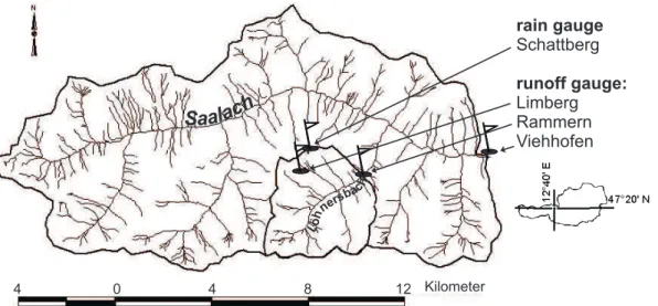
hydrogeol-ogy and stream network including saturation areas are given by Pirkl (1989)4. Rainfall runoff characteristics are monitored since 1991 by the Institute of Hydraulics, Hydrology and Water Resources Management at the Vienna University of Technology. The instru-mentation consists mainly of stream and rain gauges. Figure 1 shows the location of 5

the instrumentation relevant for this paper, namely the runoff gauges at Limberg, Ram-mern and Viehhofen and the rain gauge at Schattberg. The Viehhofen runoff gauge is operated by the Austrian Hydrographic Service, Salzburg Section.

In the L ¨ohnersbach catchment the headwater Limberg became the main field of activity at the micro-scale (Tilch et al., 2003; Kirnbauer et al., 2004b). The stream 10

gauge, at an altitude of 1780 m a.s.l., is located at the natural outlet of a saturation area. The highest point of the catchment is 2000 m a.s.l. The greatest distance between runoff gauge and catchment boundary is about 500 m. The nearest rain gauge is located outside of the catchment. The minimum distance from the headwater to the rain gauge is approximately 840 m with an elevation difference of 180 m.

15

2.2. Runoff response in the L¨ohnersbach catchment

In the L ¨ohnersbach catchment different runoff characteristics were identified (Kirnbauer et al., 1996, 2001, 2004a). The L ¨ohnersbach divides the catchment into a north-western and south-eastern part. The runoff response of both parts differs from each other. During low flow conditions, the north-western part contributes to runoff below 20

average and the south-eastern part above average. For high flow conditions and large

3

Schiffer, R. and Burgstaller, B.: Vegetationskartierung L¨ohnersbach, topical map, unpub-lished report, 1990.

4

Pirkl, H.: Erarbeitung der Zusammenh ¨ange zwischen Hanginstabilit ¨aten und -labilit ¨aten, Hangwasserhaushalt und Massenbewegungen in Teilen des Zentralalpenkristallins,

¨

Osterreichische Akademie der Wissenschaften, Geologische Bundesanstalt, Vienna, mapping, unpublished report, 1989.

HESSD

Full Screen / Esc

Print Version Interactive Discussion

EGU rain events this trend is reversed. Furthermore, different event types could be identified

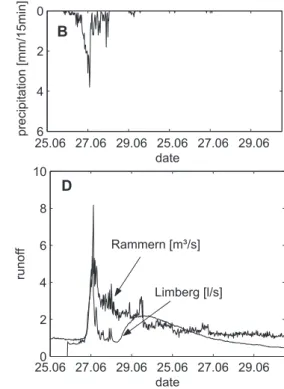
at the micro-scale (gauge Limberg) and the small-catchment scale (gauge Rammern). Figure 2 shows typical hydrographs at gauge Limberg [l/s] and at gauge Rammern [m3/s]. Direct and synchronic runoff peaks (C) occur during short and intensive rain-storms (A) at both scales. For long duration rainfall events with low rainfall intensity (B), 5

bimodal runoff events can be observed at Limberg (D). Simultaneous to the bimodal runoff events at Limberg an increased runoff volume with a slowly abating recession curve can be measured at Rammern gauge (D). Bimodal runoff response could be identified in a different headwater in the L¨ohnersbach catchment, too, and is not only a specific phenomenon of the Limberg catchment (Tilch et al., 2003). For the small-10

catchment scale (gauge Rammern), it seems quite evident that the shape of the reces-sion curve is a result of different “delayed peaks” from other locations, which occur in sum as a substantially increased hydrograph with long recession time.

2.3. Headwater Limberg

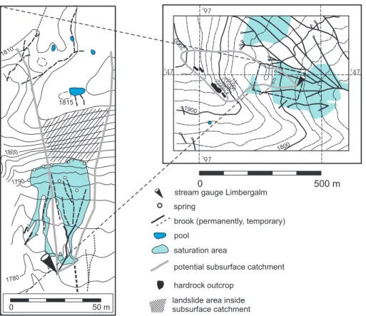
The headwater Limberg (L in Fig. 1) is located on the lateral part of a glacier. Ac-15

cordingly, the geological conditions are very complex, where subsurface flow pathways are difficult to identify. The micro-scale catchment Limberg can roughly be divided into tree major geographic-geological units (see Fig. 3). The highest unit, and furthest from the stream gauge, is a boulder field with very steep slope and a high macroporosity, underlain by low metamorphic and fractured greywake and siltstone. Downhill in more 20

flat positions is a cirque area with a frontal rim, caused by a combined rock and debris block slide. This area is characterized by thick duff layer under alpine rose vegeta-tion, some small pools and saturation areas. At the foot of the frontal rim is a saturation area fed by springs from the base of the slide mass and from inside the saturation area. Some of the springs are permanent, some are only active during wet conditions. The 25

sources providing permanent base flow are most likely supplied by additional areas from deep storage water systems.

HESSD

Full Screen / Esc

Print Version Interactive Discussion

EGU and generation areas in the headwater could be identified. This work is discussed

in detail by Tilch et al. (2003). The tracer investigations support the conclusions of Kirnbauer et al. (1996, 2001) that the unimodal peak is generated at the saturation areas and contains rain water. But pre-event water from the saturation areas could be detected in the peak flow, too. It is assumed that water, which is stored in depres-5

sions due to pasturing, gets flushed out by rain during a storm event. In the frontal rim within and under the duff layer fast episodic runoff is generated, too. After satura-tion the duff layer generates interflow. The delayed peak consists solely of pre-event water. At least two subsurface flow systems could be identified. Newer investigations (Kirnbauer et al., 2004b) prove that the water moves at least along two pathways with 10

different attenuation and storage properties (boulder field at the very steep hillslope, and the metamorphic and fractured greywake and siltstone). Unlike the delayed peak, the permanent subsurface flow comes from deeper storage systems.

3. Data and methods

3.1. Hydrograph analysis and event types 15

At Limberg scale unimodal and bimodal event types can directly be identified from the shape of the hydrograph. For all events analyzed, the same event types at the micro-scale can also be found at the Rammern and Viehhofen micro-scale. Considered character-istics are rainfall volume and intensity, initial runoff, storm runoff volume and recession constants. They are explained in detail in the following Sects. 3.3 and 3.4. To quantify 20

the runoff response the hydrographs were separated into direct storm runoff and base-flow, for which several techniques exist. In this application a straight line separation seems adequate because we wish to compare water volume mobilized by a rainfall event independent of the source area. The line was projected from the initial rise of the hydrograph to the point on the falling limb where a break in slope occurred (point 25

HESSD

Full Screen / Esc

Print Version Interactive Discussion

EGU 3.2. Rainfall runoff events

Rainfall and runoff time series of 67 storms of the years 1997–2002 were analyzed at all scales (micro-scale, small-catchment scale, meso-scale). The time series are given in intervals of 15 min. The events were taken from the period when there was no (or a negligible) snow cover and when the temperature was above 0◦C (usually 5

end of June). The beginning of an event depends on the onset of rain measured at the Schattberg gauge. An event is defined to start one time step before precipitation begins (the hydrograph rises in the same time step as rainfall occurs). The initial base flow is defined as the discharge of the first time step. It characterizes the base flow conditions before the hydrograph response to a rain impulse.

10

These 67 events, identified at the gauge Limberg, were not only analyzed at the gauge Limberg but also at the gauges Rammern and Viehhofen. It is assumed that these events affect the whole catchment up to Viehhofen with 150 km2. For the same time segments, taken at Limberg, the hydrographs measured at Rammern and Viehhofen gauge were analyzed. The beginning of an event is the same for all scales. 15

The duration of an event is taken individually according to the decay characteristics of the hydrographs at the different scales.

3.3. Event types

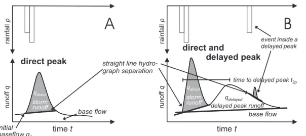
The runoff events are subdivided into unimodal and bimodal event types (Table 1). In Fig. 4 the two types measured at the Limberg gauge are drawn schematically (see 20

also Fig. 1). The unimodal event type is characterized by a peak that directly responds to the rainfall impulse. A rainfall event can have more than one impulse so that the hydrograph responds with more than one direct peak. A bimodal event consists of a direct peak response and a delayed peak as a response to the same rain impulse that initiated the direct peak.

25

In this paper storm runoff is defined as the direct response to a rainfall impulse minus base flow calculated by the straight-line separation. The delayed peak runoff

HESSD

Full Screen / Esc

Print Version Interactive Discussion

EGU volume is the volume generated in the delayed “damped” peak minus base flow volume.

For bimodal events, the onset of a delayed peak cannot be seen in the hydrograph, because the delayed peak intermixes with the direct peak reaction. We assume that the delayed peak response starts at the same time as the direct peak response. Storm runoff caused by rainfall impulses within a delayed peak were separated by straight-line 5

separation and were not included in the delayed peak runoff (see Fig. 4B). The time to delayed peak is defined as the time from the beginning of the direct peak event to the maximum discharge of the delayed peak.

3.4. Recession analysis

Recession curve analysis was used to show that unimodal and bimodal event types 10

exist not only at the micro-scale but also at the small-catchment scale and at the meso-scale. A delayed peak can only be identified as a wave-shaped hydrograph at the headwater Limberg. We hypothesize that if a delayed peak occurs at the headwater, the hydrographs at the larger scales (Rammern and Viehhofen) are characterized by significantly retarded recession. Therefore, recession coefficients were calculated for 15

all events at Rammern and Viehhofen. Two approaches were used. First, a simple and widely used method is chosen based on the assumption of a linear reservoir outflow. The runoff values of the recession limb of an event were plotted against time as a logarithmic function (Pilgrim and Cordery, 1993). If the behavior of this logarithmic function is linear, then the inverse of its slope (the inverse of the semi-20

logarithmic gradient) is equal to K_rtwith values between 0 and 1. The recession function is described by:

q_t= q₀× Kt r (1) t=time [day (86400s)] q_t=discharge [m3/s] 25 q₀=initial discharge [m3/s]

HESSD

Full Screen / Esc

Print Version Interactive Discussion

EGU K_rt=recession constant [m3×(86400s2)−1]

The log(q) values were fitted to a straight line with the coefficients a[m3×(s×86400s)−1] and b[m3/s]:

log(q)= a × t + b (2)

5

with K_rt resulting from:

K_rt= exp(a) (3)

Because various authors have shown that the storage-discharge relationship is non-linear (Kubota and Sivapalan, 1995; Wittenberg, 1999, 2003; Wittenberg and Siva-palan, 1999) a nonlinear outflow method according to Wittenberg (1999) was applied 10

to the recession curves (Eq. 4). In this case, the recession flow hydrograph was esti-mated by fitting the discharge data q_tto the non-linear storage outflow model:

q_t= q₀ 1+(1 − b) × q 1−b 0 a× b × t !b1−1 . (4)

For q_t and q₀ in [m3/s] the factor a has the dimension m3−3bsb and b is dimension-less. It has been found for numerous rivers in different hydrological regimes that b is 15

less than 1, with typical values around 0.5 (Wittenberg, 1994, 1999; Wittenberg and Sivapalan, 1999; Aksoy and Wittenberg, 2001; Mishra et al., 2003). For a fixed b, a characterizes the recession behavior of the falling limb. With increasing a, the shape of the recession limb becomes increasingly damped. To get a clear interpretable pa-rameter a, b was fixed at 0.5 and a und q₀ were fitted with a non-linear least square 20

HESSD

Full Screen / Esc

Print Version Interactive Discussion

EGU 4. Results

4.1. Runoff response of headwater Limberg

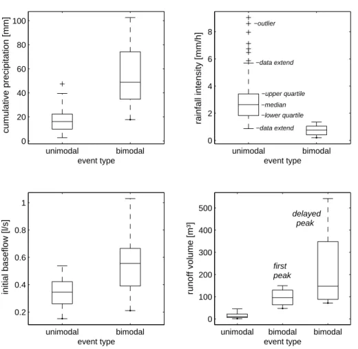
In Fig. 5 cumulative precipitation, rainfall intensity, initial baseflow and runoff volume of the two event types are compared (see also Tables 2 and 3). The bimodal events show higher cumulative precipitation, lower rainfall intensities and higher initial base 5

flow levels than the unimodal events. The runoff volume of bimodal events exceeds the runoff volume of unimodal peaks. The first peak of a bimodal event yields, compared to the unimodal peak event, more than the double runoff volume, and could be a result of the higher rainfall volume. Further, the delayed peak contributes at least half of the runoff volume of the first peak (Table 3, event 8) and can exceed the runoff of the first 10

peak up to eight times (Table 3, event 10). The bimodal events follow the same trend determined by Kirnbauer et al. (2001). For six bimodal and six unimodal events they show that the bimodal events occur under relatively high precipitation depths (greater than 40 mm), relatively low rainfall intensities (between 4 and 10 mm/h), and wet con-ditions, i.e. high initial base flow. The threshold values for bimodal runoff response 15

given by Kirnbauer et al. (2001) differ slightly from the values found here and have overlapping ranges in the case of cumulative precipitation, rainfall intensity and initial baseflow. Overall, the event characteristics at Limberg shown in Fig. 5 are statistically significantly different for both event types which was proven by the Wilcoxon test of equality of medians at a significance level of α=0.01 (99%).

20

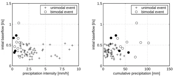
The occurrence of the two event types, unimodal and bimodal, depends on the rain-fall characteristics and on the soil moisture state of the catchment. In Fig. 6, for all 67 events, initial baseflow as indicator of the soil moisture state is plotted versus precip-itation intensity and cumulative precipprecip-itation, respectively. The two event types occur under very different event characteristics and form two separate groups (Fig. 6). A low 25

rainfall height can produce a delayed peak (Fig. 6, right), but only if the initial base-flow is high (e.g. rainfall height=17.7 mm, initial baseflow=0.67 l/s, Table 3). If the initial baseflow is low a high rainfall amount is necessary to initiate a delayed peak (e.g.

rain-HESSD

Full Screen / Esc

Print Version Interactive Discussion

EGU fall height=72.7 mm, initial baseflow=0.21 l/s, Table 3). In contrast, bimodal events

are always characterized by relative low precipitation intensities independent of initial baseflow (Fig. 6, left). It seems that the delayed peak results from an overflow of a storage system where, depending on the current water content, more or less rain input is needed to initiate a delayed peak.

5

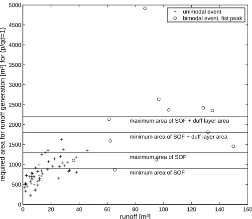
In Fig. 7 the required size of the generation area of the unimodal events and of the direct peak of the bimodal events is plotted under the assumption that the entire rain is transformed into runoff (event runoff coefficient=1). A minimum and maximum ex-tension of the saturation area of 900 and 1300 m2, respectively, was mapped during field investigations and is drawn as a line in Fig. 7. This demonstrates that the sat-10

uration area explains only the generation of runoff for small unimodal events. Other hydrological response units must generate direct runoff, too. The size of the duff layer area generating fast runoff after saturation is approximately 900 m2. However, neither saturation area nor duff layer area as an additional source of direct runoff explain all runoff events, particularly the direct peaks of the bimodal events. Further areas must 15

be involved in generating fast runoff, taking into account that the required size is cal-culated under the most unfavorable assumption of a runoff coefficient equal 1. These results are consistent with the results of Tilch et al. (2003). They could verify that the first peak does not only consist of event water from the saturation area and slide area, but also of pre-event water from the boulder field at the very steep slope.

20

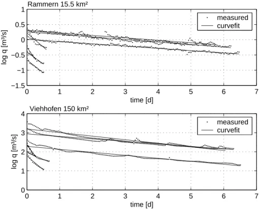
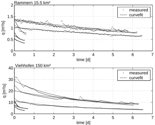
4.2. Runoff response at different scales

Figures 8 and 9 show example recession limbs for all events of 1997, with linear curve fit and q_t plotted on a logarithmic scale (Fig. 8) and with a nonlinear curve fit (Fig. 9) according to the model given by Wittenberg (1999) (see Sect. 3.4). The recession limbs are neither all concave shaped nor linear. For example, the bimodal events are 25

more linear on a log scale but unimodal events are still concave shaped (Fig. 8). In opposite, recession limbs measured at Rammern are almost linear at normal scale (Fig. 9). Hence, two methods are applied, a semi-logarithmic method assuming a

HESSD

Full Screen / Esc

Print Version Interactive Discussion

EGU linear storage-discharge relationship and the method according to Wittenberg (1999)

implying a nonlinear storage-discharge relationship.

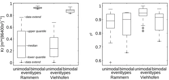
The recession coefficients K_r, calculated from the linear model (Fig. 10), and a, cal-culated from the nonlinear model (Fig. 11), are significantly different for unimodal and bimodal event types for the small-catchment scale (gauge Rammern), as well as for the 5

meso-scale (gauge Viehhofen). In both models the median r2for the goodness of curve fit are around 0.9, meaning that the fitted curves represent the runoff values q and log q very well. These results show that the event types distinguished at the headwater Limberg with a size of 0.07 km2can also be identified in the hydrographs at Rammern with a size of 15.5 km2, and at Viehhofen with a size of 150 km2. The differences can 10

be shown by the coefficients Kr and a of the linear and the nonlinear outflow model, respectively. Both models are appropriate to illustrate the different recession behavior of the unimodal and bimodal events.

The appearance of an event type at Limberg can be described by initial baseflow and cumulative precipitation (Fig. 6). Initial baseflow versus precipitation intensity, and 15

initial baseflow versus cumulative precipitation are plotted in Fig. 12 for all events for Rammern and Viehhofen scales. At both scales, the same pattern as at the micro-scale (gauge Limberg) can be observed. Again, the two event types form two separate groups. There is one exception (Fig. 12, right), namely the unimodal event at gauge Viehhofen with more then 50 mm precipitation and an initial baseflow of more than 20

12.5 m3/s. This event occurred at Viehhofen during the extreme flood event in summer 2002. But this outlier can be distinguished from the bimodal event type due to a much higher precipitation intensity.

Runoff height is plotted versus precipitation height in Fig. 13. The relationships at both scales are nonlinear and are correlated with r2=0.72 for Rammern and r2=0.82 25

for Viehhofen. Higher runoff volumes are generated during bimodal events. The runoff coefficients of the bimodal events are between 0.13 and 0.32 for Rammern and 0.24 to 0.31 for Viehhofen (Table 5), whereas unimodal events just reach a runoff coefficient of 0.07 for Rammern and 0.13 for Viehhofen, respectively (Table 4). It follows that at this

HESSD

Full Screen / Esc

Print Version Interactive Discussion

EGU scales runoff coefficients of the bimodal events are much higher than runoff coefficients

of the unimodal events, and the gap seems to increase with scale.

5. Conclusions

The results presented in this paper reveal a strong relationship between runoff re-sponse at the headwater scale (0.07 km2) and the response at larger scales (small-5

catchment scale, 15.5 km2, and meso-scale, 150 km2) in the Saalach watershed. Based on the analysis of 67 rainfall runoff events (total: 201 at three scales), two different event types could be identified at these three scales: (1) an unimodal event type, characterized by a quick rising and falling hydrograph, responding to short dura-tion rainfall, and (2) a bimodal event type, consisting of a first peak with a quick rise and 10

fall, and a second peak, when the rain has already stopped, with a much slower rise and fall. The second peak has a delay of three to 5 days. It has been shown that if a de-layed peak occurs at the gauge Limberg substantially increased flow values arise at the larger gauges Rammern and Viehhofen. For these events, the damped recession of Rammern and Viehhofen is explained by the superposition of different delayed peaks, 15

originating from different headwaters in the area. Due to diverse distances between source areas and stream gauge, and due to variable flow accumulation and flow con-centration, the overlay of several damped hydrographs results in an increased runoff of prolonged duration. This link between the scales means that the runoff behavior of the headwater (Limberg, 0.07 km2) may be used as an indicator of the runoff behavior of 20

much larger areas (Rammern, 15.5 km2, Viehhofen, 150 km2). It is interesting to note that the occurrence of the two event types is consistent over three orders of magnitude in area.

At all three scales, the occurrence of an event type depends on rainfall characteristics and initial baseflow. The bimodal events seem to result from an overflow of deeper 25

storage systems where, depending on the current water content, more or less rain input is needed to initiate a delayed peak response. During bimodal events, considerably

HESSD

Full Screen / Esc

Print Version Interactive Discussion

EGU higher runoff volume is generated at all scales. Investigations at the headwater Limberg

let come to the conclusion that the higher amount of runoff of bimodal events consists of pre-event water, generated by subsurface flow processes. This reveals that beside saturation areas subsurface compartments can be significantly involved in the flood generation process.

5

Acknowledgements. The authors would like to thank the German Science Foundation (DFG), project Me 1844/1-3, for financial support. We would also like to thank the Austrian Hy-drographic Service – Salzburg Section – for providing hyHy-drographic data for runoff gauge Viehhofen.

References

10

Aksoy, H. and Wittenberg, H.: Jahreszeitliche Ver ¨anderung der Trockenwetterganglinie – Fall-studie f ¨ur einen Fluss im europ ¨aischen Teil der T ¨urkei, Wasserwirtschaft, 90, 38–41, 2001. Anderson, M. G. and Burt, T. P.: The role of topography in controlling throughflow generation,

Earth Surface Processes, 3, 331–344, 1978.

Chapman, T.: A comparison of algorithms for stream flow recession and baseflow separation, 15

Hydrol. Processes, 13, 701–714, 1999.

Dewandel, B., Lachassagne, P., Bakalowicz, M., Weng, P., and Al, M. A.: Evaluation of aquifer thickness by analyzing recession hydrographs; application to the Oman Ophiolite hard-rock aquifer, J. Hydrol., 274, 248–269, 2003.

Gutknecht, D.: Abflussentstehung an H ¨angen – Beobachtungen und Konzeptionen, 20

¨

Osterreichische Wasser- und Abfallwirtschaft, 48, 134–144, 1996.

Grayson, R. and Bl ¨oschl, G.: Spatial processes, organisation and patterns, in: Spatial patterns in catchment hydrology. Observations and modelling, edited by: Grayson, R. and Bl ¨oschl, G., Cambridge University Press, 3–16, 2000.

Hall, F. R.: Baseflow recessions – a review, Water Resour. Res., 4, 973–983, 1968. 25

HD ¨O (Ed.): Hydrographisches Jahrbuch von ¨Osterreich 1999, Wien, Bundesministerium f ¨ur Land- und Forstwirtschaft, Umwelt und Wasserwirtschaft, 2002.

hydro-HESSD

Full Screen / Esc

Print Version Interactive Discussion

EGU chemistry: Conflicting interpretations from hydrological and chemical observations, Hydrol.

Processes, 8, 335–349, 1994.

Kirnbauer, R., Bl ¨oschl, G., Haas, P., M ¨uller, G., and Merz, B.: Identifying space-time patterns of runoff generation in the L¨ohnersbach catchment, in: Runoff generation and implications for river basin modelling, Freiburger Schriften zur Hydrologie, 13, 37–45, 2001.

5

Kirnbauer, R., Bl ¨oschl, G., Haas, P., M ¨uller, G., and Merz, B.: Identifying space-time patterns of runoff generation – A case study from the L¨ohnersbach catchment, Austrian Alps, in: Global Change and Mountain Regions, U. Huber MRHB, KLUWER academic publishers, 2004a. Kirnbauer, R., Tilch, N., Markart, G., Zillgens, B., Kohlbeck, F., Leroch, K., Seidler, C. H., Haas,

P., Uhlenbrook, S., Didszun, J., Leibundgut, C. H., Merz, B., Chawatal, W., and F ¨urst, J.: 10

Runoff generation in the northern greywack zone of the alps – field studies and mathematical modelling, Tagungsband des 10. Kongress Interpraevent in Garda 2004, 24–27 May, II, 45– 56, 2004b.

Kirnbauer, R., Pirkl, H., Haas, P., and Steidl, R.: Runoff processes; observations and modelling, ¨

Osterreichische Wasser- und Abfallwirtschaft, 48, 15–26, 1996. 15

Kirnbauer, R., Bl ¨oschl, G., Haas, P., M ¨uller, G., and Merz, B.: Identifying space-time patterns of runoff generation – A case study from the L¨ohnersbach catchment, Austrian Alps, in: Global change and mountain regions - a state of knowledge overview, edited by: Huber, U., Bugmann, H., and Reasoner, M., Springer Verlag, 309–320, in print, 2005.

Klemes, V.: Probability of extreme hydrometeorological events – a different approach, Extreme 20

Hydrological Events: Precipitation, Floods and Droughts, 213, 167–176, 1993.

Kubota, J. and Sivapalan, M.: Towards a catchment-scale model of subsurface runoff gener-ation based on synthesis of small-scale process-based modelling and field studies, Hydrol. Processes, 9, 541–554, 1995.

Masiyandima, M. C., van de Giesen, N., Diatta, S., Windmeijer, P. N., and Steenhuis, T. S.: The 25

hydrology of inland valleys in the sub-humid zone of West Africa: rainfall-runoff processes in the M’b ´e experimental watershed, Hydrol. Processes, 17, 1213–1225, 2003.

McDonnell, J. and Woods, R.: On the need for catchment classification (Editorial), J. Hydrol., 299, 2–3, 2004.

McNamara, J. P., Kane, D. L., and Hinzman, L. D.: An analysis of streamflow hydrology in the 30

Kuparuk River basin, Arctic Alaska; a nested watershed approach, J. Hydrol., 206, 39–57, 1998.

HESSD

Full Screen / Esc

Print Version Interactive Discussion

EGU hydraulic parameters of a semi-arid mountainous watershed by recession-flow analysis, J.

Hydrol., 279, 57–69, 2003.

Mishra, A., Hata, T., Abdelhadi, A. W., Tada, A., and Tanakamaru, H.: Recession flow analysis of the Blue Nile River, Hydrol. Processes, 17, 2825–2835, 2003.

Naef, F., Scherrer, S., and Weiler, M.: A process based assessment of the potential to reduce 5

flood runoff by land use change, J. Hydrol., 267, 74–79, 2002.

Nathan, R. J. and McMahon, T. A.: Evaluation of automated techniques for base flow and recession analyses, Water Resour. Res., 26, 1465–1473, 1990.

Onda, Y., Komatsu, Y., Tsujimura, M., and Fujihara, J. I.: The role of subsurface runoff through bedrock on storm flow generation, Hydrol. Processes, 15, 1693–1706, 2001.

10

Pilgrim, D. H. and Cordery, I.: Flood Runoff, in: Handbook of Hydrology, Maidment, D. R. McGraw-Hill, Inc.: 9.1–9.42, 1993.

Rodda, J. C.: Mountains – a hydrological paradox or paradise?, Beitr ¨age zur Hydrologie der Schweiz, 41–51, 1994.

Rose, S. and Peters, N. E.: Effects of urbanization on streamflow in the Atlanta area (Georgia, 15

USA): A comparative hydrological approach, Hydrol. Processes, 15, 1441–1457, 2001. Singh, V. P. and Strupczewski, W. G.: On the status of flood frequency analysis, Hydrol.

Pro-cesses, 16, 3737–3740, 2002.

Sujono, J., Shikasho, S., and Hiramatsu, K.: A comparison of techniques for hydrograph reces-sion analysis, Hydrol. Processes, 18, 403–413, 2004.

20

Tallaksen, L. M.: A review of baseflow recession analysis, J. Hydrol., 165, 349–370, 1995. Tilch, N., Uhlenbrook, S., Didszun, J., Leibundgut, C., Zillgens, B., Kirnbauer, R., and Merz, B.:

Decoding flow formation processes using tracer hydrologic methods in an Alpine catchment, ¨

Osterreichische Wasser- und Abfallwirtschaft, 55, 9–17, 2003.

Uhlenbrook, S., Frey, M., Leibundgut, C., and Maloszewski, P.: Hydrograph separations in a 25

mesoscale mountainous basin at event and seasonal timescales, Water Resour. Res., 38, 1096, 2002.

Vitvar, T., Gurtz, J., and Lang, H.: Application of GIS-based distributed hydrological modelling for estimation of water residence times in the small Swiss pre-alpine catchment Rietholzbach, IAHS-AISH-Publication, 258, 241–248, 1999.

30

Viviroli, D., Weingartner, R., and Messerli, B.: Assessing the hydrological significance of the world’s mountains, Mountain Res. Dev., 23, 32–40. 2003.

HESSD

Full Screen / Esc

Print Version Interactive Discussion

EGU runoff? A combined tracer and runoff transfer function approach, Water Resour. Res., 39,

11, 1315, doi:10.1029/2003WR002331, 2003.

Weingartner, R., Barben, M., and Spreafico, M.: Floods in mountain areas – an overview based on examples from Switzerland, J. Hydrol., 282, 10–24, 2003.

Wetzel, K. F.: Runoff production processes during different rainfall in small hillslope catchments 5

of the northern limestone Alps, Erde, 132, 361–379, 2001.

Wittenberg, H.: Nonlinear analysis of flow recession curves, IAHS Publication, 221, 61–67, 1994.

Wittenberg, H.: Baseflow recession and recharge as nonlinear storage processes, Hydrol. Processes, 13, 715–726, 1999.

10

Wittenberg, H.: Effects of season and man-made changes on baseflow and flow recession; case studies, Hydrol. Processes, 17, 2113–2123. 2003.

Wittenberg, H. and Sivapalan, M.: Watershed groundwater balance estimation using stream-flow recession analysis and basestream-flow separation, J. Hydrol., 219, 20–33, 1999.

HESSD

Full Screen / Esc

Print Version Interactive Discussion

EGU

Table 1. Number of runoff events for the two event types.

year unimodal event bimodal event time period

1997 5 3 22 June–13 Sept. 1998 13 1 27 June–28 Sept. 1999 13 4 21 June–28 Sept. 2000 8 2 10 July–3 Oct. 2001 7 2 16 June–8 Aug. 2002 9 – 27 June–10 Sept. total 55 12

HESSD

Full Screen / Esc

Print Version Interactive Discussion

EGU

Table 2. Characteristics of the unimodal events measured at the headwater Limberg.

55 events t_e[d] p [mm] p_i [mm/h] p_i−max q₀[l/s] qs [m3]

median 0.41 16.1 2.63 10 0.35 10.69

minimum value 0.11 2.7 0.86 2 0.15 1.16

maximum value 2.32 74.4 9.04 44 0.54 45.71

t_e, event duration; p, total rainfall; pi, precipitation intensity; qi−max, maximum precipitation

HESSD

Full Screen / Esc

Print Version Interactive Discussion

EGU

Table 3. Characteristics of the bimodal events measured at the headwater Limberg.

event start t_e q₀ t_2p p_direct p_i p_i−max qs_direct qs_delayed [d] [l/s] [d] [mm] [mm/h] [mm/h] [m3] [m3] *1 22 June 1997 15.02 0.73 3.35 28.7 0.60 1.2 61.32 71.55 2 5 July 1997 17.69 0.55 4.90 102.6 1.35 5.5 149.75 160.87 3 17 July 1997 20.69 0.56 4.80 84.8 1.12 2.3 94.93 245.51 *4 7 July 1998 26.42 0.36 5.05 36.7 0.45 3.9 96.77 542.02 *5 21 June 1999 20.83 0.67 5.81 17.7 0.20 3.1 86.98 93.54 6 9 July 1999 24.09 0.46 8.30 39.1 0.37 4.4 62.21 112.65 7 22 July 1999 21.00 0.57 5.27 53.0 0.66 9.1 128.27 133.62 *8 26 Aug. 1999 26.29 0.32 10.80 57.2 0.32 2.1 134.80 75.07 9 10 July 2000 20.83 0.42 5.49 43.8 0.85 1.1 103.78 420.01 10 5 Aug. 2000 16.67 0.66 3.70 32.7 0.88 2.7 47.27 387.62 11 16 June 2001 14.71 1.03 4.08 75.5 0.98 2.0 65.40 309.33 12 19 July 2001 20.83 0.21 4.86 72.7 1.14 2.6 131.701 82.85

t_e, event duration; q₀, initial baseflow; t_2p, time to second peak; p_direct, rainfall during direct peak duration; pi, rainfall intensity; qi−max, maximum precipitation intensity; qsdirect, storm runoff from

direct peak, qs_delayed, storm runoff from delayed peak

HESSD

Full Screen / Esc

Print Version Interactive Discussion

EGU

Table 4. Characteristics of the unimodal events measured at gauges Rammern and Viehhofen.

Rammern Viehhofen t_e q₀ qs qs/p t_e q₀ qs qs/p [d ] [m3/s] [m3/km2] [-] [d ] [m3/s] [m3/km2] [-] median 0.53 0.49 291 0.02 0.79 3.64 635 0.040 minimum value 0.17 0.26 9 0.004 0.25 1.87 23 0.005 maximum value 1.56 1.0 3361 0.07 2.52 12.51 6438 0.130

HESSD

Full Screen / Esc

Print Version Interactive Discussion

EGU

Table 5. Characteristics of the bimodal events measured at gauges Rammern and Viehhofen.

Rammern Viehhofen event start t_e q₀ qs qs/p t_e q₀ qs qs/p [d ] [m3/s] [m3/km2] [-] [d ] [m3/s] [m3/km2] [-] *1 22 June 1997 7.51 0.77 5871 0.17 7.51 5.15 8413 0.25 2 5 July 1997 8.84 0.70 17 185 0.13 9.19 3.18 42 749 0.27 3 17 July 1997 10.34 0.70 14 772 0.13 10.34 7.47 33 663 0.29 *4 7 July 1998 13.21 0.70 26 126 0.23 13.21 5.49 32 318 0.29 *5 21 June 1999 – – – 10.42 6.86 16 340 0.31 6 9 July 1999 – – – 11.32 5.08 16 132 0.28 7 22 July 1999 – – – 11.22 4.96 21 462 0.24 *8 26 Aug. 1999 15.28 0.46 8464 0.21 15.95 3.55 16 317 0.24 9 10 July 2000 10.41 0.42 23 032 0.32 10.42 3.80 17 143 0.25 10 5 Aug. 2000 8.75 0.81 17 020 0.32 8.75 6.87 15 154 0.29 11 16 June 2001 7.77 0.67 11 262 0.14 7.77 8.90 20 198 0.26 12 19 July 2001 10.83 0.31 15 426 0.20 10.70 2.21 18 162 0.25 t_e, event duration; q₀, initial baseflow; qs, storm runoff; qs/p, runoff coefficient

HESSD

Full Screen / Esc

Print Version Interactive Discussion EGU Kilometer 4 0 4 8 12

w

w

w

w

Saala

ch

Fig. 1. Map of the nested study area of the upper Saalach basin: upper Saalach (150 km2, gauge Viehhofen), L ¨ohnersbach (15.5 km2, gauge Rammern), and Limberg (0.07 km2, gauge Limberg).

HESSD

Full Screen / Esc

Print Version Interactive Discussion EGU 25.06 27.06 29.06 25.06 27.06 29.060 2 4 6 8 10 date runof f Rammern [m³/s] Limberg [l/s] 01.070 03.07 05.07 07.07 2 4 6 8 10 date runof f Rammern [m³/s] Limberg [l/s] C D 25.06 27.06 29.06 25.06 27.06 29.06 date 01.07 03.07 05.07 07.07 date precipit ation[mm/15min] precipit ation[mm/15min]

Fig. 2. Typical hydrographs of the micro-scale catchment at stream gauge Limberg and

meso-scale catchment at stream gauge Rammern: direct and synchronic runoff peaks (C) during short and intensive rainstorms(A), and bimodal runoff events (D) during and after moderate

HESSD

Full Screen / Esc

Print Version Interactive Discussion EGU 1817 1780 1790 1800 1810 1815 1815 0 500 m spring

potential subsurface catchment brook (permanently, temporary) pool

hardrock outcrop saturation area

stream gauge Limbergalm

2 47 3₉₇ 3 97 1800 1900 20 00 2₄₇

landslide area inside subsurface catchment

0 50 m

Fig. 3. Headwater catchment Limberg with stream network, saturation areas, ponds and

HESSD

Full Screen / Esc

Print Version Interactive Discussion EGU direct peak time t storm runoff

base flow _{base flow}

delayed peak direct and

delayed peak runoff

storm runoff

rainfall

p

straight line hydro-graph separation

event inside a delayed peak

time t

A

B

time to delayed peak t_2p

runof fq initial baseflow q0 qdelayed qdirect qdirect rainfall p runof fq

Fig. 4. Schematic representation of the hydrographs of an unimodal peak event (A) and a

HESSD

Full Screen / Esc

Print Version Interactive Discussion EGU unimodal bimodal 0.2 0.4 0.6 0.8 1 initial baseflow [l/s] event type unimodal bimodal 0 2 4 6 8 rainfall intensity [mm/h] event type −outlier −data extend −upper quartile −median −lower quartile −data extend unimodal bimodal 0 20 40 60 80 100 cumulative precipitation [mm] event type

unimodal bimodal bimodal

0 100 200 300 400 500 runoff volume [m³] event type delayed peak first peak

Fig. 5. Comparison of cumulative precipitation, rainfall intensity, initial baseflow and runoff

volume for unimodal and bimodal events. (The whiskers of the box plots extend to the minimum and maximum data value, however, not more than 1.5*interquartile range).

HESSD

Full Screen / Esc

Print Version Interactive Discussion EGU 0 2.5 5 7.5 10 0 0.5 1 1.5 precipitation intensity [mm/h] initial baseflow [l/s] 0 50 100 150 0 0.5 1 1.5 cumulative precipitation [mm] initial baseflow [l/s] unimodal event bimodal event unimodal event bimodal event

Fig. 6. Hydrological characteristics of the two event types (unimodal and bimodal) of the

micro-scale catchment, stream gauge Limberg (filled circles indicate bimodal events with underpre-dicted precipitation due to errors in time series).

HESSD

Full Screen / Esc

Print Version Interactive Discussion EGU 0 20 40 60 80 100 120 140 160 0 500 1000 1500 2000 2500 3000 3500 4000 4500 5000 runoff [m³]

required area for runoff generation [m²] for (p/qd=1)

minimum area of SOF maximum area of SOF

minimum area of SOF + duff layer area maximum area of SOF + duff layer area

unimodal event bimodal event, fist peak

Fig. 7. Required area to generate the observed runoff volume of the first peak of bimodal events

and of the unimodal events, under the assumption that the event runoff coefficient equals 1 (SOF: saturation area).

HESSD

Full Screen / Esc

Print Version Interactive Discussion EGU 0 1 2 3 4 5 6 7 0 1 2 3 4 time [d] log q [m³/s] Viehhofen 150 km² 0 1 2 3 4 5 6 7 −1.5 −1 −0.5 0 0.5 1Rammern 15.5 km² time [d] log q [m³/s] measured curvefit measured curvefit

Fig. 8. Recession curves for the rainfall runoff events measured 1997 (every forth measured

HESSD

Full Screen / Esc

Print Version Interactive Discussion EGU 0 1 2 3 4 5 6 7 0 10 20 30 40 Viehhofen 150 km² time [d] q [m³/s] 0 1 2 3 4 5 6 7 0 0.5 1 1.5 2Rammern 15.5 km² time [d] q [m³/s] measured curvefit measured curvefit

Fig. 9. Recession curves for the rainfall runoff evens measured 1997 (every forth measured

HESSD

Full Screen / Esc

Print Version Interactive Discussion

EGU

unimodal bimodal unimodal bimodal 0 0.2 0.4 0.6 0.8 1 Kr [m³*(86400s²) − 1 ] eventtypes eventtypes Rammern Viehhofen

unimodal bimodal unimodal bimodal 0.6 0.7 0.8 0.9 1 r² eventtypes eventtypes Rammern Viehhofen −data extend −upper quantile −median −lower quantile −data extend

Fig. 10. Box plots of recession coefficients Kr (left) with goodness of curve fit r 2

(right) for the unimodal and bimodal event types at the small-catchment scale (gauge Rammern) and at the meso-scale (gauge Viehhofen).

HESSD

Full Screen / Esc

Print Version Interactive Discussion

EGU

unimodal bimodal unimodal bimodal 0 5 10 15 20 a [m (3 − 3 b ) *s b ] eventtypes eventtypes Rammern Viehhofen

unimodal bimodal unimodal bimodal 0.6 0.7 0.8 0.9 1 r² data extend− upper quantile− median− lower quantile− data extend− outlier− eventtypes eventtypes Rammern Viehhofen

Fig. 11. Boxplots of coefficient a (left) calculated with the nonlinear model with goodness of

curve fit r2(right) for the two event types at the small-catchment scale (gauge Rammern) and at the meso-scale (gauge Viehhofen).

HESSD

Full Screen / Esc

Print Version Interactive Discussion EGU 0 5 10 0 0.5 1 1.5 precipitation intensity [mm/h] initial baseflow [m³/s] 0 50 100 150 0 0.5 1 1.5 initial baseflow [m³/s] cumulative precipitation [mm] 0 5 10 0 5 10 15 precipitation intensity [mm/h] initial baseflow [m³/s] 0 50 100 150 0 5 10 15 initial baseflow [m³/s] cumulative precipitation [mm] bimodal event unimodal event Rammern 15.5 km² Rammern 15.5 km² Viehhofen 150 km² Viehhofen 150 km²

Fig. 12. Initial base flow versus cumulative precipitation, and initial baseflow versus

precipi-tation intensity, for gauge Rammern and Viehhofen (filled circles indicate bimodal events with underpredicted precipitation due to errors in time series).

HESSD

Full Screen / Esc

Print Version Interactive Discussion EGU 0 50 100 150 200 0 10 20 30 40 50 cumulative precipitation [mm] runoff [mm] y=0.0012x2.0063 r²=0.72 Rammern 15.5 km² 0 50 100 150 200 0 10 20 30 40 50 cumulative precipitation [mm] runoff [mm] y=0.0027x1.9261 r²=0.82 Viehhofen 150 km² unimodal event bimodal event

Fig. 13. Runoff volume versus cumulative precipitation for direct peak events and for bimodal

events at three different scales (total runoff from bimodal events is the runoff from both peaks, filled circles indicate bimodal events with underpredicted precipitation due to errors in time series).