HAL Id: hal-02399661
https://hal.archives-ouvertes.fr/hal-02399661v2
Submitted on 3 Dec 2020HAL is a multi-disciplinary open access archive for the deposit and dissemination of sci-entific research documents, whether they are pub-lished or not. The documents may come from teaching and research institutions in France or abroad, or from public or private research centers.
L’archive ouverte pluridisciplinaire HAL, est destinée au dépôt et à la diffusion de documents scientifiques de niveau recherche, publiés ou non, émanant des établissements d’enseignement et de recherche français ou étrangers, des laboratoires publics ou privés.
Grigorii Kokhanenko, Yuri Balin
To cite this version:
Antonin Zabukovec, Gérard Ancellet, Jacques Pelon, Iogannes Penner, Grigorii Kokhanenko, et al.. Identification of Aerosol Sources in Siberia and Study of Aerosol Transport at Regional Scale by Airborne and Space-Borne Lidar Measurement. EPJ Web of Conferences, EDP Sciences, 2020, 237, 02014 (4 p.). �10.1051/epjconf/202023702014�. �hal-02399661v2�
I
DENTIFICATIONOF AEROSOLSOURCES INS
IBERIAANDSTUDYOF AEROSOL TRANSPORTATREGIONAL SCALEBY AIRBORNE ANDSPACE-
BORNELIDARMEASUREMENT
Antonin Zabukovec1, Gérard Ancellet1, Jacques Pelon1, J.D. Paris2, Iogannes E. Penner3, Grigorii
Kokhanenko3, Yuri S. Balin3
1 Laboratoire Atmosphere Milieux, Observations Spatiales (LATMOS), CNRS, Sorbonne Université,
Université Versailles St Quentin, Paris, France
2Laboratoire des Sciences du Climat et de l’Environnement, CEA-CNRS-UVSQ, Gif sur Yvette, France
3 Zuev Institute of Atmospheric Optics, Russian Academy of Sciences, Tomsk, Russia
ABSTRACT
Airborne lidar measurements were carried out over Siberia in July 2013 and June 2017. Aerosol optical properties are derived using the Lagrangian FLEXible PARTicle dispersion model (FLEXPART) simulations and Moderate Resolution Imaging Spectrometer (MODIS) AOD. Comparison with Cloud-Aerosol Lidar with Orthogonal Polarization (CALIOP) aerosol products is used to validate the CALIOP aerosol type identification above Siberia. Two case studies are discussed : a mixture of dust and pollution from Northern Kazakhstan and smoke plumes from forest fires. Comparisons with the CALIOP backscatter ratio show that CALIOP algorithm may overestimate the LR for a dusty mixture if not constrained by an independent AOD measurement.
1. INTRODUCTION
Asian pollution and oil/gas flaring in Siberia have been identified as aerosol key sources, however the impact by these pollutants is poorly known. CALIOP or MODIS satellite observations provide valuable information about aerosol spatial distributions and optical properties may be compared with ground-based or airborne observations. Regional aerosol studies with CALIOP have been conducted for high latitudes [1], European Arctic [2], or the Arctic ice sheet [3], but no similar studies exist for Central Siberia.
2. METHODOLOGY
2.1 Objectives and methodology
Airborne backscatter lidar observations in Siberia were carried out and compared to CALIOP data
using Level 2 Version 4 CALIOP aerosol data products [4] and Level 1 CALIOP attenuated backscatter processed at LATMOS [2] in order to assess CALIOP aerosol optical properties accuracy.
Aerosol types were characterized using the Lagrangian FLEXPART model, aircraft in-situ measurements, MODIS AOD and CALIOP aerosol vertical extent and depolarization in the source region. Biomass-burning emissions were identified using the daily fire radiative power (FRP) maps based on NASA Fire Information for Resource Management System (FIRMS) using MODIS [5] and the Visible Infrared Imaging Radiometer Suite (VIIRS) [6]. Only FRP > 0,05 GW were taken into account.
2.2 Aircraft campaigns
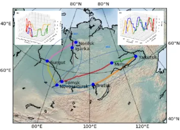
The aircraft campaigns took place in July 2013 and June 2017. The four flight tracks for each campaign are shown in Fig 1.
Fig. 1: Map of the 8 aircraft flight tracks carried
loop). The aircraft altitude ranges are also shown for the 2017 (b) and 2013 (c) flights.
The flights were selected to fly over (i) the major Siberian cities (Novosibirsk, Tomsk, Krasnoyarsk, Yakutsk) (ii) the gas flaring fields of the Ob valley and the industrial city of Norilsk (iii) the Siberian taiga to sample long-range transport of forest fires and mid-latitude Eastern Asia emissions.
2.3 Airborne lidar system
The transmitter module is based on a solid state Nd-YAG laser emitting 8 ns laser pulse at 532 nm. The optical receiver is a 150 mm diameter tion lens coupled with a 1nm filter and two recep-tion channels (co- and cross-polarizarecep-tion). The vertical sampling is less than 6 m. The full geo-metrical overlap is obtained between 80m and 150m. In practice the first 200 m are not used to account for lidar misalignment during the flights. The cross-polarization calibration is not good enough to characterize the aerosol type and is mainly used to discriminate cloud and aerosol lay-ers.
2.4 Aerosol optical depth retrieval
The lidar calibration is performed several times during each flight using a normalization of the at-tenuated backscatter signal (PR2) to molecular backscatter in the range 200m-700m below the aircraft when the fit with the molecular density slope is better than 4%, only at altitudes above 3.5 km and when no aerosol/cloud layers are seen in the calibration range. The vertical profile of molecular backscatter was estimated from the 0.75° ERA-Interim ECMWF meteorological anal-ysis.
Aerosol optical depth retrieval is based on the Fernald forward inversion of the calibrated PR2 [7]
,
assuming a range independent value of aerosol lidar ratio (LR). The LR value is constrained using the distribution of 10 km MODIS collection 6 aerosol optical depth (AOD) in an area of ± 70 km and a time lag of ± 5 h around the aircraft observation.The distribution of possible LR values was recursively tuned to obtain an airborne lidar AOD within the 25th and 75th percentile of the MODIS AOD distribution. To estimate the uncertainty of the retrieved backscatter ratio, 500 inversions
were randomly performed using the LR distribution and using a backscatter coefficient distribution at the reference altitude according to the estimated calibration error.
3. RESULTS
3.1 Urban pollution case
During the 2017 campaign, between Novosibirsk and Surgut above the Ob Valley, the aerosol vertical distribution shows 100-200 km horizontal layers in the 0 and 2.5 km altitude range (Fig. 2).
Fig. 2: Vertical cross-section of airborne lidar
log10(PR2) on June, 16 2017 . Calibration constant is 13458 ± 2%. Grimm aerosol concentrations in particle.cm-3 are shown at the aircraft altitude. The FLEXPART simulation (Fig. 3) potential emission sensitivity (PES) is used to identify the possible aerosol sources (PES > 2000 s). Both aerosol emissions from the Novosibirsk area and from Kazakhstan can explain the layers seen by the airborne lidar.
Fig. 3: Map of the PES distribution for
FLEXPART backward simulation for the aerosol layers between 0-2 km at 56.6°N Fig. 2 (black
cross). The pink dotted lines are the selected CALIOP overpasses in the source area.
MODIS AOD and tropospheric CO column measured by IASI are however higher in Northern Kazakhstan (0.15-025 AOD, 2.0-2.5 x10¹⁸ molecule.cm-2 CO column) than in the Novosibirsk area (0.05-0.12 AOD, 1.5-1.8 x10¹⁸ molecule.cm-2 CO column).
No forest fires are located in the high PES areas according to the FIRMS data. A CALIPSO vertical cross-section above Northern Kazakhstan shows depolarizing aerosol layers (> 10%) up to 3km altitudes between 45°N and 50°N (Fig. 4). A mixture of dust and pollution source is then expected in the layers seen by the airborne lidar at 56°N, 80°E.
Fig. 4: Vertical cross-section of CALIOP 532
backscatter coefficient (right side) on June 16 in the Kazakhstan source region. CALIOP 532 depolarization ratio vertical profile at 49.74°N (left side).
The mean airborne lidar backscatter ratio at 56.7°N is 19 ± 0.1 below 2.5 km altitude with an AOD532 of 0.0895 ± 0.0225 and LR between 26 and 40, when constrained by MODIS observations (Fig. 5). The corresponding aerosol type would be “dusty mix” according to [8]. It is also in good agreement with the FLEXPART analysis.
Two CALIOP backscatter ratio profiles in the same area at 55.5°N, 82.5°E on June 15th, 21 UT and at 57°N, 87°E on June 17th, 20 UT are in good agreement with the airborne lidar observations. The correspondingAOD532 are 0.1 ± 0.04 (0.1 ± 0.04) and 0.168 ± 0.062 (0.139 ± 0.047) for the CALIOP L2 product (LATMOS processed L1 data) on June 15th and 17th respectively, with LR between 55 and 70 sr. A better match with the airborne lidar and MODIS
AOD could be obtained by using LR values smaller than 40 as expected for a dusty mix type.
Fig. 5: (a) 50 km average of the backscatter ratio
vertical profile for the airborne lidar on June 16th 05 UT (green), CALIOP on June 15th (blue) and on June 17th (red). (b) MODIS AOD
550 distribution in the ± 70 km area around the aircraft.
3.1 Boreal forest fire case
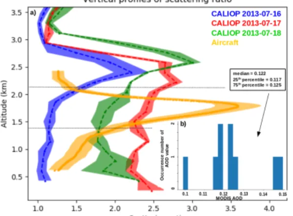
During the 2013 campaign, a 500 m thick aerosol layer is observed by the airborne lidar at 2.0 km between Tomsk and Mirnyy (Fig.6).
Fig. 6: Vertical cross-section of aircraft log10(PR2) on July, 19 2013. Calibration constant is 491724 ± 10%. Grimm aerosol concentrations in parti-cle.cm-3 are shown at the aircraft altitude.
According to the FLEXPART simulation, no aerosol transport is expected from large cities or pollution sources, while several forest fires were identified by the FIRMS data close to the aircraft position (Fig. 7). The mean airborne lidar backscatter ratio at 58°N (Fig. 6) is larger than 3.0
between 1.5 and 2.2 km altitude with an AOD532 of 0.122 ± 0.022 and LR between 53 and 56, when constrained by MODIS observations. Such values are consistent with a “fresh smoke” aerosol type according to [8].
Fig. 7: Map of the PES distribution for
FLEX-PART backward simulation for the aerosol layer at 1.7 km Fig. 6 (black cross). The red dots are FIRMS forest fires and the pink dotted lines are the selected CALIOP overpasses in the source area.
Fig. 8: (a) 20 km average of the backscatter ratio
vertical profile from the airborne lidar on July 19th 6 UT (yellow), CALIOP on July 16th 19 UT (blue), on July 17th 19 UT (red) and on June 18th 5 UT (green). (b) MODIS AOD550 distribution in the ± 70 km area around the aircraft position. This backscatter ratio profile can be compared with several CALIOP tracks observed near forest fires in the same area (Fig. 7). The CALIOP verti-cal profiles show smoke layers between 2km and 3 km altitude, but with backscatter ratio between 2 and 3 (Fig. 8). CALIOP AODs in the latitude band 60°N-62°N range from 0.1 to 0.3 with lidar ratio
of 70 sr. AODs are also in good agreement with the range of MODIS AOD around the CALIOP tracks. While the airborne lidar is able to sample fresh smoke layer, CALIOP profiles did not over-pass fires during the combustion phase and are thus mainly representative of fire plumes after transport and mixing. It explains both the vertical structure of the CALIOP aerosol layers (larger thicknesses and smaller peak values) and larger li-dar ratio for aged biomass plume [8].
Conclusion and Perspectives
During the 2017 and 2013 aircraft campaigns, mixed layers of dust and pollution from Northern Kazakhstan and smoke layers in forest area were detected by the airborne lidar. Comparison with CALIOP backscatter ratio shows that CALIOP al-gorithm may overestimate the LR for a dusty mix-ture if not constrained by an independent AOD measurement. The use of low liquid water cloud reflectance from the Synergized Optical Depth of Aerosols product (SODA) or land surface re-flectance from the Wide Field Camera (WFC) aboard CALIOP could be a step forward to derive the aerosol CALIOP extinction above Siberia.
ACKNOWLEDGEMENTS
This work was supported by Sorbonne Université and the French Centre National d’Etudes Spa-tiales.
REFERENCES
[1] M.Di. Pierro, and al. Atmospheric Chemistry and Physics 11.5, 2225-2243 (2011)
[2] G. Ancellet, and al. Atmospheric Chemistry and Physics 14.16, 8235-8254 (2014)
[3] C. Di Biagio, and al. Journal of Geophysical Research: Atmospheres 123.2, 1363-1383 (2018) [4] M.H. Kim, and al. Atmospheric Measurement Techniques 11.11 (2018)
[5] L. Giglio, and al. Remote Sensing of Environ-ment 87.2-3 , 273-282 (2003)
[6] W. Schroeder, and al. Remote Sensing of Envi-ronment 143, 85-96 (2014)
[7] F. Fernald, et al. Applied Optics 23.5, 652-653 (1984)
[8] S.P. Burton, et al. Atmospheric Measurement Techniques 6.5, 1397-1412 (2013)