Proposing a mechanistic understanding of changes in atmospheric CO<sub>2</sub> during the last 740 000 years

(1)

HAL Id: hal-00298121

https://hal.archives-ouvertes.fr/hal-00298121

Submitted on 14 Feb 2006

HAL is a multi-disciplinary open access

archive for the deposit and dissemination of sci-entific research documents, whether they are pub-lished or not. The documents may come from teaching and research institutions in France or abroad, or from public or private research centers.

L’archive ouverte pluridisciplinaire HAL, est destinée au dépôt et à la diffusion de documents scientifiques de niveau recherche, publiés ou non, émanant des établissements d’enseignement et de recherche français ou étrangers, des laboratoires publics ou privés.

Proposing a mechanistic understanding of changes in

atmospheric CO2 during the last 740 000 years

P. Köhler, H. Fischer

To cite this version:

P. Köhler, H. Fischer. Proposing a mechanistic understanding of changes in atmospheric CO2 during the last 740 000 years. Climate of the Past Discussions, European Geosciences Union (EGU), 2006, 2 (1), pp.1-42. �hal-00298121�

(2)

CPD

2, 1–42, 2006

Simulating pCO₂ during the last

740 kyr

P. K ¨ohler and H. Fischer

Title Page Abstract Introduction Conclusions References Tables Figures J I J I Back Close

Full Screen / Esc

Print Version Interactive Discussion

EGU Climate of the Past Discussions, 2, 1–42, 2006

www.climate-of-the-past.net/cpd/2/1/ SRef-ID: 1814-9359/cpd/2006-2-1 European Geosciences Union

Climate of the Past Discussions

Climate of the Past Discussions is the access reviewed discussion forum of Climate of the Past

Proposing a mechanistic understanding

of changes in atmospheric CO

₂

during the

last 740 000 years

P. K ¨ohler and H. Fischer

Alfred Wegener Institute for Polar and Marine Research, P.O. Box 12 01 61, 27 515 Bremerhaven, Germany

Received: 15 December 2005 – Accepted: 20 January 2006 – Published: 14 February 2006 Correspondence to: P. K ¨ohler (pkoehler@awi-bremerhaven.de)

(3)

CPD

2, 1–42, 2006

740 kyr

Full Screen / Esc

EGU Abstract

Atmospheric carbon dioxide (CO₂) measured in Antarctic ice cores shows a natural variability of 80 to 100 ppmv during the last four glacial cycles and variations of ap-proximately 60 ppmv in the two cycles between 410 and 650 kyr BP. We here use dust and the isotopic temperature proxy deuterium (δD) from the EPICA Dome C Antarctic 5

ice core covering the last 740 kyr together with other paleo-climatic records to force the ocean/atmosphere/biosphere box model of the global carbon cycle BICYCLE in a forward mode over this time in order to reconstruct the natural variability of pCO₂. Our simulation results covered by our proposed scenario are based on process un-derstanding gained previously for carbon cycle variations during Termination I. These 10

results match the pCO₂measured in the Vostok ice core well (r2=0.80) and we predict prior to Termination V significantly smaller amplitudes in pCO₂variations mainly based on a reduced interglacial ocean circulation and reduced interglacial Southern Ocean sea surface temperature. These predictions for the pre-Vostok period match the new pCO₂ data from the EPICA Dome C ice core for the time period 410 to 650 kyr BP 15

equally well (r2=0.79). This is the first forward modelling approach which covers all major processes acting on the global carbon cycle on glacial/interglacial time scales. The contributions of different processes (terrestrial carbon storage, sea ice, sea level, ocean temperature, ocean circulation, CaCO₃chemistry, marine biota) are analysed.

1. Introduction

20

Paleo-climatic records derived from ice cores revealed the natural variability in Antarc-tic temperature (Jouzel et al.,1987), atmospheric dust content (R ¨othlisberger et al., 2002), and atmospheric CO₂ (Barnola et al., 1987; Fischer et al., 1999; Petit et al., 1999; Monnin et al., 2001; Kawamura et al., 2003; Siegenthaler et al., 2005) over the last glacial cycles. The longest CO₂ record from the Antarctic ice core at Vos-25

(4)

CPD

2, 1–42, 2006

740 kyr

Full Screen / Esc

EGU (410 kyr BP) showing a switch of glacials and interglacials in all those parameters

ap-proximately every 100 kyr during the last four glacial cycles with pCO₂varying between 180–300 ppmv. New measurements of dust and the isotopic temperature proxy δD of the EPICA Dome C ice core covered the last 740 kyr, however, revealed glacial cy-cles of reduced temperature amplitude (EPICA community members, 2004). These 5

new archives offer the possibility to propose atmospheric CO2for the pre-Vostok time span as called for in the EPICA challenge (Wolff et al., 2004). Here, we contribute to this challenge using a box model of the isotopic carbon cycle (K ¨ohler et al.,2005) based on process understanding previously derived for Termination I and show that major features of the Vostok period are reproduced while prior to Termination V our 10

model predicts significantly smaller amplitudes in pCO₂ variations. These pre-Vostok prediction are matched for the time interval 410–650 kyr BP by the new pCO₂data set measured at EPICA Dome C (Siegenthaler et al.,2005).

The quest of explaining the observed glacial/interglacial variations in atmospheric pCO₂ of about 80–100 ppmv (Petit et al., 1999) was challenging the scientific com-15

munities for at least two decades (e.g.Archer et al.,2000;Sigman and Boyle,2000). Processes which need to be included in solving this quest are the transport of or-ganic and dissolved inoror-ganic carbon (DIC) from the surface to the deep ocean via its physical and biological pumps. Large changes in vertical mixing of the water col-umn (Toggweiler,1999), changes in the strength of the thermohaline circulation (THC) 20

(Knorr and Lohmann, 2003), variations in sea ice cover in high latitudes limiting gas exchange rates (Stephens and Keeling, 2000; Archer et al., 2003) together with well known temperature and salinity variations (Adkins et al.,2002) of the ocean are pro-cesses affecting the carbon cycle via the physical pump. The fertilisation of the marine biological productivity through the aeolian input of iron in areas of high nitrate and low 25

chlorophyll is one theory (Martin, 1990; Ridgwell, 2003) which would reduce atmo-spheric pCO₂ during glacial times through an enhanced biological export production to the deep ocean. The export of organic carbon itself is closely coupled to the cal-cium carbonate production of pelagic calcifiers by which CO₂is released in the surface

(5)

CPD

2, 1–42, 2006

740 kyr

Full Screen / Esc

EGU ocean. Additionally to those processes which distribute DIC, alkalinity and nutrients in

the different ocean reservoirs, exchange fluxes of carbon between the terrestrial bio-sphere and the ocean/atmobio-sphere system (e.g.Joos et al.,2004), riverine input of bi-carbonate (Munhoven,2002), and exchange fluxes of DIC and alkalinity via dissolution and sedimentation between ocean and sediments (Zeebe and Westbroek,2003) need 5

to be considered to fully understand glacial/interglacial changes in the global carbon cycle.

Previously we put forward a quantitative explanation of observed changes in atmo-spheric pCO₂ and its carbon isotopes (δ13C, ∆14C) using the multi-box model of the global carbon cycle, called BICYCLE, applied to the last glacial termination (K ¨ohler 10

et al.,2005). That study concluded that the main processes impacting on pCO₂ dur-ing Termination I were an increase in vertical mixdur-ing rates in the Southern Ocean and changes in the DIC and alkalinity inventories through sedimentation and dissolution processes. The time-dependent atmospheric δ13C record from the Taylor Dome ice core (Smith et al.,1999) used in that study contains valuable informations, which en-15

abled us to reduce the uncertainties in determining the magnitude and timing of various processes. These results are in that sense robust that the detailed magnitudes of indi-vidual processes might vary due to model limitation and data uncertainties, but all their contributions need to be taken into account for explaining the observed variations in the atmospheric carbon records. The still limited knowledge on the size of a marine glacial 20

iron fertilisation effect in the Southern Ocean might be named as largest uncertainty, however, a recent data compilation (Kohfeld et al.,2005) on the role of marine biology on glacial/interglacial CO₂cycles supports our approach that as a net effect the South-ern Ocean marine export production might be a glacial sink for carbon. Assuming that these processes are of general nature, we apply in the following the same model over 25

the time period of the last 740 kyr covered by the EPICA Dome C records to predict pCO₂ variations over the EPICA Dome C era. To this end we forced our model by proxy data from marine and ice core archives.

(6)

CPD

2, 1–42, 2006

740 kyr

Full Screen / Esc

EGU

2. Methods

2.1. The BICYCLEmodel

The Box model of the Isotopic Carbon cYCLE BICYCLE (K ¨ohler et al.,2005) was de-veloped and applied for quantitative interpretation of the atmospheric carbon records (pCO₂, δ13C, ∆14C) during Termination I (10−20 kyr BP). The model consists of ten 5

oceanic reservoirs in three different depth layers and distinguishes Atlantic, Indo-Pacific and Southern Ocean (Fig. 1). The strength of the preindustrial ocean circulation as seen in Fig. 1 was parameterised with data from WOCE (Ganachaud and Wunsch, 2000). Marine global export production of 10 PgC yr−1at 100 m water depth ( Gnanade-sikan et al.,2002) was prescribed for the preindustrial setting, depending on the pre-10

formed macro-nutrient concentration of PO₄ in the surface waters. In the equatorial regions all macro-nutrients were utilised for the export production, while in the high lat-itudes the export production flux was restricted to avoid a global export flux of carbon which exceeds the prescribed 10 PgC yr−1. This led to unutilised nutrient concentra-tions especially in the Southern Ocean, which can be used for increased marine pro-15

ductivity during times of high aeolian iron input into these regions. The rain ratio of DIC to CaCO₃in the export production fluxes was kept constant at 10:1 throughout all our simulations. As another boundary condition describing sediment/ocean interactions the lysocline was either kept constant or its variation is prescribed, both leading to fluxes of DIC and alkalinity in the ratio of 1:2 between the deep ocean and the sediments. 20

In doing so we mimic the dissolution or sedimentation of CaCO₃ in the absence of a process-based module of early diagenesis (e.g. Archer et al., 2000). This approach calculates the net changes in the inventories of DIC and alkalinity and therefore implic-itly includes changes in the weathering inputs of bicarbonate through rivers. A globally averaged seven-compartment terrestrial biosphere (K ¨ohler and Fischer,2004) allows 25

photosynthetic production of C₃ and C₄ pathways differing in their isotopic fractiona-tion, and a climate and CO₂-dependent fixation of carbon on land. A more detailed

(7)

CPD

2, 1–42, 2006

740 kyr

Full Screen / Esc

EGU description of the model is found inK ¨ohler et al.(2005).

2.2. Time-dependent forcing of BICYCLE

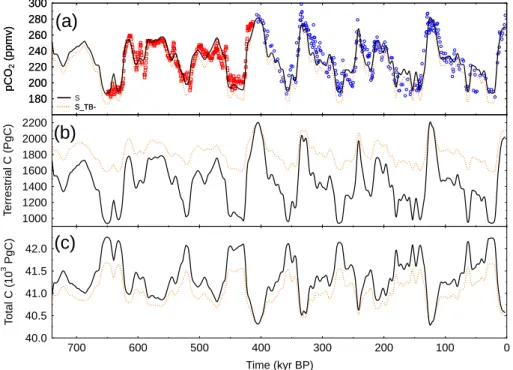
We forced BICYCLE forward in time using various paleo-climatic records (Fig. 2). The

model applied here used the same parameterisation as for its application on Termi-nation I (K ¨ohler et al., 2005) with the two exceptions that (1) we did not consider a 5

complete shut-down of the North Atlantic Deep Water (NADW) formation during Hein-rich events and (2) we selected two scenarios for terrestrial carbon storage which span the range found in the literature. The first change (NADW) is based on productivity results (Sachs and Anderson, 2005) and sea level fluctuations (Siddall et al.,2003) that indicate that Heinrich events during MIS 2 and 3 may have caused different per-10

turbations to the ocean circulation. It is therefore not possible to generalise changes in NADW formation throughout the EPICA Dome C period. Nevertheless, we discuss the potential impact of Heinrich events in Sect.3.2. The second change was performed to highlight the error propagation of the still existing uncertainties in the glacial/interglacial rise in carbon stored on land onto atmospheric pCO₂.

15

Because various records that were used to force our model had a rather coarse resolution we have chosen to smooth all forcing records and all simulation results and concentrate on low frequency changes in the carbon cycle.

The relevant forcing functions were adapted as follows:

Ocean temperature: Reconstructed summer SST at ODP980 (McManus et al.,1999; 20

Wright and Flower,2002) (using modern analogue techniques in the times before 500 kyr (Wright and Flower,2002)) was used as proxy for SST changes in the North At-lantic (north of 50◦N) scaled to a glacial/interglacial amplitude during Termination I of 4 K (Fig. 2b). SSTs of equatorial surface oceans were estimated from planktic δ18O measured in ODP677 in the equatorial Pacific (Shackleton et al., 1990) scaled to a 25

glacial/interglacial amplitude during Termination I of 3.75 K (Visser et al.,2003) which was already used previously (Fig.2d). Southern Ocean (south of 40◦S) SST with a glacial/interglacial amplitude during Termination I of 4 K was estimated from δD of the

(8)

CPD

2, 1–42, 2006

740 kyr

Full Screen / Esc

EGU EPICA Dome C ice core (EPICA community members,2004) (Fig. 2h). Here, EPICA

Dome C δD was corrected for the effect of sea level changes (Jouzel et al.,2003) using a normalised record of sea level change fromBintanja et al.(2005).

Sea ice: Varying sea ice coverage will influence the gas exchange rates between the

atmosphere and the surface ocean. We coupled time-dependent changes in the sea 5

ice area in the North Atlantic and the Southern Ocean on the assumed temperature changes in the respective surface ocean boxes. Present day annual mean sea ice area was set to 10×1012m2 in each hemisphere (Cavalieri et al.,1997). During the LGM the annual average area covered by sea ice increased to 14×1012m2in the North and 22×1012m2 in the South based on various studies (Crosta et al.,1998a,b;Sarnthein 10

et al.,2003;Gersonde et al.,2005). In addition to changing surface box area due to sea level change this results in a relative areal coverage of 50 and 85% in the North Atlantic box and 13 and 30% in the Southern Ocean box during preindustrial times and the LGM, respectively.

Sea level: We used the results of Bintanja et al. (2005) on changes in sea level 15

(Fig. 2f). This modelling study is based on a benthic δ18O stack from 57 globally distributed sediment core covering more than the last 5 million years (Lisiecki and Raymo,2005).

Ocean circulation: There are data- and model-based evidences for a reduced ocean

overturning in the Atlantic and the Southern Ocean, while the glacial circulation in the 20

Pacific Ocean seemed to have been similar to todays (Meissner et al., 2003; Hodell et al.,2003;Knorr and Lohmann,2003;Broecker et al.,2004;McManus et al.,2004; Watson and Garabato,2006). It was shown (Flower et al.,2000) that the depth gradient in δ13C which is an indicator for the strength in NADW formation is highly correlated with benthic δ18O. To rely on as few different cores as possible and thus to minimise 25

timing uncertainties we therefore used benthic δ18O in ODP980 (McManus et al.,1999; Flower et al.,2000) as a proxy for the strength in NADW formation bearing in mind that this might introduce a possible phase shift of the contribution of changes in NADW formation on pCO₂(Fig.2c). We defined δ18ONADW=2.8‰ as a threshold for changes

(9)

CPD

2, 1–42, 2006

740 kyr

Full Screen / Esc

EGU in the Atlantic thermohaline circulation. The strength of NADW formation of 16 Sv

(1 Sv=106m3s−1) during interglacial periods (δ18O<2.8‰) was based on the World Ocean Circulation Experiment WOCE (Ganachaud and Wunsch,2000), the strength of 10 Sv during glacial times (δ18O≥2.8‰) on various modelling studies (e.g. Meiss-ner et al.,2003). The net vertical water mass exchange fluxes in the Southern Ocean 5

was coupled linearly to Southern Ocean temperature changes with 29 Sv during prein-dustrial SST and 9 Sv during the LGM. Southern Ocean deep water ventilation would also be reduced due to the glacial reduction of NADW formation by 6 Sv and its sub-sequent fluxes. An instantaneously switching from glacial to interglacial mixing rates in the Southern Ocean as used previously (K ¨ohler et al.,2005) was not necessary here 10

due to the low resolution of all forcing records. Changing ocean circulation fluxes are depicted in bold in Fig.1.

Marine biota: Due to the prescribed export production fluxes in our reference sce-nario there exist unutilised macro-nutrients in the Southern Ocean surface waters. In these high nutrient low chlorophyll areas an increased export production in times of 15

high aeolian iron input might occur as described in the iron fertilisation hypothesis (Martin, 1990; Ridgwell, 2003). The atmospheric dust content of the EPICA Dome C ice core (EPICA community members,2004) was used as proxy for aeolian input of iron into the Southern Ocean which might enhance marine biological productivity there if allowed by macro-nutrient availability (Fig. 2i). We keep a similar threshold 20

(dust_Fe>310 ppbv) as deduced for Termination I (K ¨ohler et al.,2005) above which iron fertilisation might occur. Increased export production was then coupled linearly to in-creased dust concentrations.

Terrestrial biosphere: The changing terrestrial carbon storage depends on the

inter-nally calculated CO₂concentration (CO₂fertilisation) and average global temperature, 25

the latter calculated as 3:1 mixture of northern and southern hemispheric tempera-ture with glacial/interglacial amplitudes of 8 and 4 K, respectively (K ¨ohler and Fischer, 2004; K ¨ohler et al., 2005). Temperature changes were forced by simulation results from Bintanja et al. (2005) for the North, who calculated the average northern (40–

(10)

CPD

2, 1–42, 2006

740 kyr

Full Screen / Esc

EGU 80◦N) hemispheric temperature changes as a function of sea level variations and

thus northern land ice sheet distribution based on the stacked benthic δ18O record of Lisiecki and Raymo(2005) (Fig.2e), and by EPICA Dome C δD for the South (Fig.2h). Glacial/interglacial fluctuations in terrestrial carbon is with about 1000 PgC at the up-per range predicted by various modelling and data based studies (see review inK ¨ohler 5

and Fischer,2004). Alternative smaller glacial/interglacial changes in terrestrial carbon storage are investigated in a sensitivity study.

CaCO₃chemistry: All changes in the carbon cycle alter the concentration of the CO2−₃

ion in the deep ocean. As a consequence the saturation horizon of CaCO₃ varies, which then induces changes in either the dissolution or sedimentation rates, a pro-10

cess known as CaCO₃ compensation (Broecker and Peng, 1987). In the absence of a process-based model of early diagenesis, which would cover these processes, we here calculated sediment/deep ocean fluxes of calcium carbonate (changing deep ocean DIC and alkalinity in a ratio of 1:2) by the application of an additional bound-ary condition. We forced our model to reconstruct observed variations in the temporal 15

changes of the lysocline. The lysocline is the oceanic depth below which sedimentary calcite dissolves and is approximated in our model with the saturation depth of calcite, which is calculated as a function of depth (pressure) in vertical steps of 200 m and in-terpolated in-between. The variations in the depth of the Pacific lysocline were derived from CaCO₃preservation of 17 cores located between 3903 and 4949 m water depth 20

(Farrell and Prell,1989) (Fig.2g). The lysocline in the Atlantic and the Southern Ocean was in a first step assumed to be constant, while later on variations in these two ocean basins on our results were investigated. This approach covers changes in the net fluxes of DIC and alkalinity, and thus implicitly includes riverine inputs of bicarbonate through weathering (Munhoven,2002).

(11)

CPD

2, 1–42, 2006

740 kyr

Full Screen / Esc

EGU 3. Results

3.1. Reconstruction of low frequency changes in atmospheric pCO₂

The simulation results of atmospheric pCO₂ in our standard scenario (Fig. 2j) show high correlations with both the Vostok (r2=0.80 in the time window 0–410 kyr BP) and the EPICA Dome C (r2=0.79; 410–650 kyr BP) pCO2 records (Petit et al.,1999; 5

Siegenthaler et al.,2005). Our model reproduces the natural variability in pCO₂ranging from 180 ppmv during glacial maxima to 260 ppmv in the interglacial periods between Marine Isotope Stage (MIS) 13 and 17 and 280 ppmv during the last four interglacials. The agreement in terms of timing and amplitude of changes is especially remarkable during terminations, but fails to reproduce some features of the data records:

10

(A) The timing in the simulation of pCO₂ reductions during some glaciations is incor-rect. This might be largely caused by an earlier decrease in the Antarctic ice core temperature proxies δD than in the Southern Ocean sea surface temperature (SST). From the deuterium excess record in the ice (Vimeux et al.,2002) it is known that the temperature change in the source regions of the precipitated moisture lags Antarctic 15

temperature during glaciations.

(B) We fail to reproduce the pCO₂ maxima of 300 ppmv in MIS 9. As our model is driven by various paleo-climatic archives plotted on their individual age scales and of low temporal resolution (∼1 kyr) especially the reproduction of peak values in pCO₂ depends on the temporal matching of these driving records. Therefore, our results 20

here have to be understood as an estimate of low frequency fluctuations in pCO₂. Furthermore, coral reef growth which increases pCO₂ during sea level high stands (Vecsei and Berger, 2004) is not considered so far leaving space for interpretation during interglacial times in which sea level rose above 70 m below present and the main shelfs were flooded.

25

(C) A major excursion between simulation and data at 150–180 kyr BP occurs at times of high fluctuations in the atmospheric dust content crossing several times the thresh-old which indicates the start in iron fertilisation in the Southern Ocean (Fig.2i). This

(12)

CPD

2, 1–42, 2006

740 kyr

Full Screen / Esc

EGU simple parametrisation of iron fertilisation is responsible for the third mismatch

indicat-ing the limitations of our approach here. The consequences of this simple approach are analysed in detail in our sensitivity study in the next subsection.

(D) Finally, our simulations do not reconstruct fast fluctuations in pCO₂as seen in the EPICA Dome C pCO₂record in MIS 15 around 600 kyr BP. At least 20–30 ppmv, about 5

half of the amplitudes seen in the pCO₂ record, can be explained, if a more accurate and higher resolved record of EPICA Dome C δD (J. Jouzel et al., unpublished data) for the earlier parts of the ice core record is taken for forcing the model. The uncertainty in the age model in this time period (Brook,2005) might also be responsible for parts of the offset.

10

In the pre-Vostok period covered by EPICA Dome C (for which pCO₂data were not available during the call of the EPICA challenge) both the regularity and the amplitude in atmospheric pCO₂as proposed with our model differ from those of the Vostok period (Fig. 2j). Peak values during interglacial periods in MIS 13, 15, and 17 reach 250– 260 ppmv, with 70 to 120 kyr elapsing in-between. Atmospheric pCO₂ drops during 15

glacials in MIS 12, 14, and 16 to 180–200 ppmv.

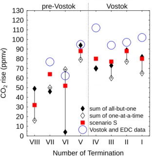
Our simulations suggest that the smallest glacial/interglacial rise in pCO₂of 50 ppmv occured from MIS 14 to MIS 13 across Termination VI, about half of the amplitudes which are simulated across the Terminations I to V; the impact of Termination VII on pCO₂ seemed to have been of average magnitude (Fig. 3). The tendency of cooler 20

and longer interglacials as seen in the EPICA Dome C δD data (EPICA community members,2004) is also mirrored by our proposed pCO₂record. According to our model the pCO₂ concentration in the pre-Vostok period remained longer at relatively high levels, but with smaller glacial/interglacial amplitudes compared to the Vostok period. Again, the low frequency variations as seen in the new EPICA Dome C pCO₂ record 25

are matched by our standard scenario very well.

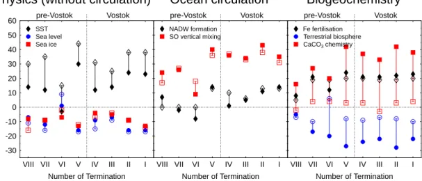
In two sensitivity analyses the importance of individual processes were investigated by (a) excluding one process from time-dependent forcings (Fig.4) and (b) forcing only one process at a time (Fig. 5). From these analyses we estimate the contributions

(13)

CPD

2, 1–42, 2006

740 kyr

Full Screen / Esc

EGU of individual processes to the rise in pCO₂ during the last eight terminations (Fig. 6)

keeping in mind the limited validity of the absolute values due to the high non-linearities of the simulated system. The contributions (estimated by excluding one process from time-dependent forcings) in decreasing order to the rise in pCO₂are given by changes in exchange fluxes between ocean and sediment (on average 38 ppmv during Termi-5

nation I to V and 21 ppmv earlier), Southern Ocean vertical mixing (38/20 ppmv), iron fertilisation in the Southern Ocean (22/14 ppmv), ocean temperature (21/8 ppmv), and NADW formation (9/−1 ppmv). Changes in sea level (−13/−6 ppmv), gas exchange caused by sea ice cover (–9/–8 ppmv), and terrestrial carbon storage (–25/–14 ppmv) were processes enlarging the observed pCO₂ rise by up to 50 ppmv during termina-10

tions. While most processes are reduced in their magnitude prior to Termination V, the absolute contribution of iron fertilisation changes only slightly. Thus, the relative im-portance of biogeochemical processes including CaCO₃ chemistry is enhanced from 45% to 60% during earlier terminations. The contribution of physical processes (SST, sea level, sea ice) to the pCO₂rise during terminations stays always below 20%, while 15

ocean circulation contributed on average 50% during the Vostok period (including Ter-mination V), but only 30–40% during TerTer-mination VII (Fig.6).

In the single process analysis follwing the one-at-a-time approach (Fig.5, Fig.6) one has to keep in mind two limiations regarding the contributions from the terrestrial carbon stocks and from the CaCO₃chemistry. (1) Carbon storage on land is itself a function of 20

atmospheric pCO₂through the CO₂fertilisation of photosynthesis. Therefore, in a sin-gle process analysis variations in terrestrial carbon storage depict only those changes caused by the change in global temperature, but not by the CO₂ concentration. The pCO₂ variations in Fig. 5TB are based on a glacial/interglacial variation in terrestrial carbon storage of about 130 PgC, and not of more than 1000 PgC as simulated in our 25

standard scenario. (2) The estimation of CaCO₃chemistry processes on the changes in pCO₂in the one-at-a-time approach (Fig. 5CA, Fig. 6) finds only a contribution of several ppmv (<5 ppmv), which derives from of the change in the depth of the lyso-cline. In simulations in which all other processes acting on the carbon cycle are also

(14)

CPD

2, 1–42, 2006

740 kyr

Full Screen / Esc

EGU operating the CaCO₃chemistry responses to deep ocean CO2−₃ concentration and the

impact on atmospheric pCO₂is one order of magnitude larger.

As mentioned byBrook(2005) the EDC2 age model (Schwander et al.,2001) which has been used for all EPICA Dome C records here, might need a revision in the times covering MIS 13 to 15. Our simulations point in the same direction: In general, sea 5

level maxima occur during warm interglacial periods, while sea level minima fall to-gether with minimum temperatures. This is the case for the sea level reconstruction based on benthic δ18O data (Bintanja et al.,2005) and δD from EPICA Dome C for the last 450 kyr (Fig.2). During MIS 13 to 15 these two records are out of phase, which is probably caused by chronological uncertainties in the EPICA Dome C records caused 10

by anomalies in ice flow. An updated chronology correcting for these mismatches is currently developed (F. Parrenin et al., unpublished manuscript). The implication of this chronological artefact in the Dome C data sets is, that our reconstruction of pCO₂ across Termination VI is biased. For example, the contribution from sea level rise dur-ing Termination VI is positive, opposdur-ing its signal durdur-ing all other glacial/interglacial 15

transitions (Fig.6). This leads also to a very small estimate of the pCO₂ during Ter-mination VI in the sum of all processes estimated from the sensitivity analysis which excluds one process from time-dependent forcings (Fig.3).

Termination VIII has also to be taken with caution as EPICA Dome C δD data prior to 740 kyr BP (J. Jouzel et al., unpublished data) reveal that minimum temperatures and 20

thus full glacial conditions in MIS 18 are reached in even older times. 3.2. Model sensitivity

Our approach proposes a decline of pCO₂ by ∼10 ppmv during terminations con-tributed by changes in the gas exchange rate through the shrinking of sea ice coverage. This would contradict a previous modelling study (Stephens and Keeling,2000) which 25

concluded that a nearly full sea ice coverage of the Southern Ocean south of 55◦S would reduce pCO₂ by 67 ppmv. Although the reliability of this previous study was

(15)

CPD

2, 1–42, 2006

740 kyr

Full Screen / Esc

EGU questioned because of the proposed very high sea ice coverage (Morales-Maqueda

and Rahmstorf,2001) the question remains why our model responses in the opposite direction. It was already shown (Archer et al.,2003) that a model response to a fully Southern Ocean sea ice coverage is highly model depending. In our study the rise in pCO₂ during deglaciations is caused by larger gas exchange rate in the North At-5

lantic Ocean which itself is caused by the decrease in the northern sea ice cover. As the modern North Atlantic is a sink for CO₂while the Southern Ocean is a source, re-ducing gas exchange during glacials in the North is increasing the glacial atmospheric pCO₂. The net effect of sea ice coverage in the Southern Ocean is negligible and reaches the magnitude of the North only when the Southern Ocean surface box is 10

nearly fully covered by sea ice (Fig. 7). However, our data based assumption pro-poses only an average annual glacial sea ice coverage of 30% in our Southern Ocean surface box. We therefore have to acknowledge that this effect is model dependent. Furthermore, in our single process analysis we consider only the effect of sea ice on gas exchange rates, while in the previous studies the overall effect of sea ice on both 15

gas exchange and ocean circulation schemes was analysed. Measurements on gas exchange through sea ice of different temperature come to the conclusions, that gas exchange is not totally prevented by a complete sea ice cover, (Gosink et al.,1976; Semiletov et al.,2004). Therefore, we believe that the impact of sea ice cover on the global carbon cycle is not yet fully understood.

20

In our reference scenario we have chosen to keep NADW formation unchanged dur-ing Heinrich events as there are evidences from productivity (Sachs and Anderson, 2005) and sea level (Siddall et al.,2003) reconstructions, that the impact may differ. Here, we estimate the maximum impact through a complete shut-down of NADW for-mation during Heinrich events identified by ice rafted debris (IRD) in the North Atlantic 25

sediment record ODP980 measured on the same core than two other paleo records used already in our study (North Atlantic SST and benthic δ18O) (McManus et al., 1999; Wright and Flower, 2002). IRD in percentage of sediment grains larger than 150 µm (relative IRD) is a proxy for the occurrence of Heinrich events (Heinrich,1988).

(16)

CPD

2, 1–42, 2006

740 kyr

Full Screen / Esc

EGU We used the relative strength IRDH=10% as threshold indicating large iceberg and

thus freshwater discharges occurring in the North Atlantic which result in a complete shut-down of the NADW formation during glacial times in our model. This threshold was derived from the analysis of IRD and known Heinrich events during the last glacial cycle (Heinrich, 1988). During two time intervals relative IRD data were missing in 5

ODP980 (740–700 and 543–500 kyr BP). The absolute IRD record (lithics/g) spanned our whole simulation period (Wright and Flower, 2002) and showed no major excur-sions in the incomplete periods of the relative IRD record apart from one large peak during the period 740–700 kyr BP. However, this absolute record is unsuitable for the predictions of Heinrich events as known events occurring during the last glacial cycle 10

(Heinrich,1988) would have been overestimated. IRD in a second core approximately 1000 km apart (ODP984) shows similar features during 500−740 kyr BP (Wright and Flower,2002) suggesting an at least regional distribution of the IRD signals measured in ODP980 and the changes in freshwater discharge indicated by them.

A shut-down of the NADW formation occurring during the Heinrich events, which 15

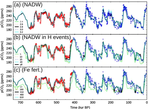
were identified by the relative IRD record, reduces atmospheric pCO₂ during glacial climate conditions by about 10 ppmv (Fig. 4). Only a Heinrich event around 550 kyr BP happening during intermediate climate conditions would lead to a sharp drop in pCO₂ by more than 30 ppmv. The selection criteria for Heinrich events (IRDH=10%) was varied in a sensitivity study (Fig.8b), and showed rather unchanged response of 20

pCO₂ for a threshold increase by a factor of two, and an extension of Heinrich events if IRD_Hwas lowered.

The impacts of the other two thresholds on modelled processes (δ18O_NADW in ODP980 as regulator for the strength of NADW formation; dust_Fe in EPICA Dome C as indicator for iron fertilisation in the Southern Ocean) were also tested (Fig.8). The 25

strength in the NADW formation during interglacial times depends to a certain extent on the chosen threshold which indicates a switch from glacial to interglacial circulation patterns in the Atlantic Ocean (Fig. 8a). The NADW formation strength during warm periods around 200 kyr BP and in the pre-Vostok time is only switching into its

(17)

inter-CPD

2, 1–42, 2006

740 kyr

Full Screen / Esc

EGU glacial mode (16 Sv), when the threshold parameter is increased leading to a rise in

pCO₂ by about 10 ppmv. The impact of Southern Ocean iron fertilisation on pCO₂ (Fig.8c) varies only if its dependency on EPICA Dome C dust content is altered by one order of magnitude and during the high dust fluctuations around 150−180 kyr BP. We therefore consider our results during 150−180 kyr BP to be influenced by our approach 5

of simulating iron fertilisation and as fairly robust otherwise.

It was argued recently that based on the knowledge gained from experiments only 0.5 to 15% of the the glacial/interglacial rise in pCO₂ can be caused by iron fertilisa-tion of the marine biota (de Baar et al.,2005). However, their estimate was based on the assumption that the glacial aeolian iron input into the Antarctic region was 11-fold 10

its modern flux, while data from EPICA Dome C find increases in iron fluxes (Wolff et al.,2006) and non-sea salt dust fluxes (R ¨othlisberger et al.,2002) from interglacial to glacial periods by a factor of 25. We therefore believe that the implications of iron fertilisation experiments for questions of glacial/interglacial pCO₂ rise do not limit the impact of iron onto the global carbon cycle in the way as proposed by de Baar et al. 15

(2005). With this different interpretation our simulation results, which propose a contri-bution of this process of approximately 25%, are still within the range covered by iron fertilisation experiments (1–34%).

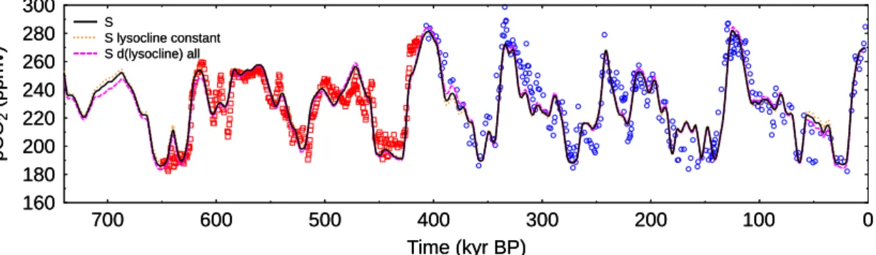
It is known that the depth variations of the lysocline in the Atlantic and the Southern Ocean were opposing those trends seen in the Pacific Ocean (Curry and Lohmann, 20

1986;Crowley,1983;Howard and Prell,1994). Due to missing data sets of lysocline variations in these two ocean basins over the whole simulation period the lysocline in the Atlantic and the Southern Ocean was kept constant in our standard simulation. We tested the importance of this simplification by further sensitivity scenarios, in which either all lysoclines were kept constant, or all were varied similar to the Pacific data set 25

ofFarrell and Prell(1989) (Fig.9). Atmospheric pCO₂variations are less than 5 ppmv different in these additional simulations than in our standard scenario. This implies, that the calculation of exchange fluxes of DIC and alkalinity itself to counterbalance changes in deep ocean CO2−₃ concentration is very important, but the precise knowledge of the

(18)

CPD

2, 1–42, 2006

740 kyr

Full Screen / Esc

EGU lyscoline is of minor relevance in the model.

To cover the estimated range in the glacial/interglacial rise in terrestrial carbon stor-age of 300–1100 PgC (K ¨ohler and Fischer,2004) an alternative scenario S TB- with reduced variability of the terrestrial biosphere was investigated. Terrestrial carbon stor-age varies during Termination I by about 500 PgC in S TB- and 1100 PgC in the stan-5

dard scenario S (Fig.10b). The change in the amplitude in terrestrial carbon storage leads also to different CaCO3 fluxes between sediment and deep ocean and thus to different fluctuations in the overall carbon budget. While total carbon of the simulated ocean-atmosphere-biosphere system is 1700 PgC larger in the LGM if compared with preindustrial times in scenario S, this glacial carbon rise is reduced to 1200 PgC in 10

scenario S TB- (Fig.10c). This additional carbon during glacial conditions enters the simulated system from the sediments. As overall effect glacial atmospheric pCO2 is about 15 ppmv lower in scenario S TB- than in S (Fig.10a). Our scenarios cover a large part of the range of changes in terrestrial carbon storage proposed by different studies. The overall impact of different terrestrial carbon storage on pCO2is small. 15

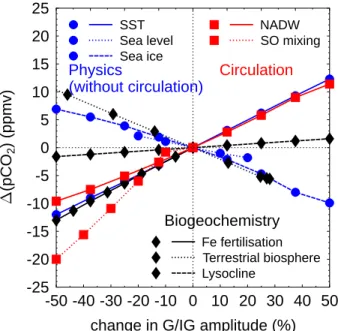
Finally, we investigated the sensitivity of our model to the amplitudes in these eight different processes contributing to the glacial/interglacial pCO2rise. We therefore var-ied their glacial/interglacial amplitudes by up to ±50% from their standards and com-pared the relative impacts on pCO₂ for Termination I (Fig. 11). The sensitivity of the modelled pCO₂ to changes in the amplitude of one process is rather linear. Varying 20

amplitudes by less than 20% would result in less than ∼5 ppmv deviation in pCO₂. We therefore evaluate our model as rather robust to the detailed knowledge of individual processes.

4. Discussion

Our study proposes a mechanistic understanding of the global carbon cycle which en-25

ables us to reconstruct low frequency changes in the natural carbon cycle on glacial timescales. The simulation results match atmospheric pCO₂ during the last 650 kyr

(19)

CPD

2, 1–42, 2006

740 kyr

Full Screen / Esc

EGU rather well (r2∼0.8) and we propose pCO2 variations back to 740 kyr BP to be

con-firmed by future measurements of pCO₂enclosed in air bubbles in Antarctic ice cores. The novelty of our approach is the fact that the process understanding how the global carbon cycle including its isotopes is operating during Termination I seems to be suf-ficient to explain atmospheric pCO₂ not only during the regular variations observed in 5

the Vostok ice core but also to predict correctly smaller glacial/interglacial amplitudes prior to Termination V. The application of our model to this long timescales is in a way a confirmation that our assumptions made for and our understanding gained from a detailed reconstruction during Termination I (K ¨ohler et al.,2005) are not restricted to this very narrow time window, but are of general nature.

10

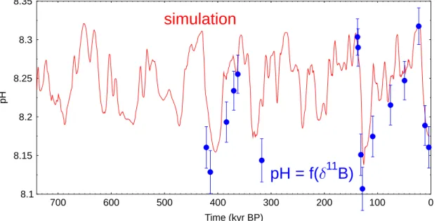
Our results are further supported by reconstructed pH in the equatorial Atlantic surface waters, which are based on δ11B measurements from planktic foraminifers (H ¨onisch and Hemming,2005). As we calculate the whole carbonate system in our model, we are able to compare our simulated pH variations in the surface water box of the equatorial Atlantic with these measurements (Fig. 12). Although the data set 15

is very sparse (16 data points over two glacial cycles) our model predicts a similar glacial/interglacial amplitude of 0.15 in this area. Minima during interglacial periods are smaller in the data than in the model. The difference between simulation and data during MIS 9 (∼330 kyr BP) are very probably caused by our simulation results, as we are also unable to reconstruct pCO₂ very accurately here. For the other differences 20

it is so far not clear if they are caused by local effects recorded in δ11B or model un-certainties. The reorganisation of the carbon cycle during interglacial periods such as the Holocene, in which pCO₂ varied by about 20 ppmv (Inderm ¨uhle et al., 1999) is not within the scope of this work. Various alternative scenarios based on data anal-ysis and more complex models were already proposed for the interpretation of the 25

Holocene pCO₂record (e.g.Broecker et al.,2001;Brovkin et al.,2002;Ridgwell et al., 2003;Ruddiman,2003;Joos et al.,2004;Wang et al.,2005). Further details on carbon cycle variations during the last glacial cycle, for which more and more accurate pCO₂

(20)

CPD

2, 1–42, 2006

740 kyr

Full Screen / Esc

EGU data exist, are found in K ¨ohler et al. (2006)1.

To our knowledge, there exist so far two transient modelling approaches which try to explain atmospheric pCO₂ during the late Pleistocene both using conceptual mod-els (Gildor et al., 2002; Paillard and Parrenin, 2004) and concentrate on changes in ocean physics. These two approaches differ widely, one (Gildor et al., 2002) being 5

purely theoretically and trying to explain the typical amplitude and seesaw shape of pCO₂ observed in Vostok, while the other (Paillard and Parrenin,2004) is forced by insolation over the last 1000 kyr. However, both pinpoint reduced glacial vertical mix-ing in the Southern Ocean as one mechanism which contributes significantly to the glacial/interglacial rise in pCO₂. While we here support the importance of changes in 10

Southern Ocean vertical mixing, we also want to point out that especially those pro-cesses which modify the overall budgets of DIC and alkalinity in the ocean need some considerations (Archer et al.,2000) and a restricted view onto the ocean/atmosphere carbonate system only is of limited validity for a complete understanding of the ob-served changes in the carbon cycle as recorded in the ice cores.

15

One result of the EPICA challenge was that all approaches using exisiting Antarctic temperature proxies and simple regression functions were able to predict pCO₂ with high accuracy (Wolff et al., 2005). Can we understand this coupling of atmospheric pCO₂ and Antarctic/Southern Ocean temperature from our process-based modelling approach? SST of the Southern Ocean itself is according to our model responsible 20

for half of the rise in pCO₂caused by ocean temperature, which would be ∼15 ppmv during Termination I. Changes in sea ice cover and Southern Ocean vertical mixing are

in BICYCLE functions of Southern Ocean SST, causing 0 ppmv and 35 ppmv,

respec-tively. As discussed earlier the contribution of Southern Ocean sea ice cover is model dependent and should therefore be taken with caution. Furthermore, CaCO₃ compen-25

1

K ¨ohler, P., Muscheler, R., and Fischer, H.: A model-based interpretation of low frequency changes in the carbon cycle during the last 120 kyr and its implications for the reconstrucion of atmospheric∆14C and the geomagnetic field strength, Geochemistry, Geophysics, Geosys-tems, in review, 2006.

(21)

CPD

2, 1–42, 2006

740 kyr

Full Screen / Esc

EGU sation is a responding process on changes in deep ocean CO2−₃ concentration. Let

us assume that its contribution of 40 ppmv to the simulated rise of 80 ppmv might be linearly coupled to perturbations in the carbon cycle caused by other processes. Taken all the mentioned processes together (direct effect of Southern Ocean SST: 15 ppmv; indirect effects: 35 pmmv; CaCO3amplifier: 50/80×40 ppmv=25 ppmv) we are able to 5

explain already a rise in pCO₂of 75 ppmv during Termination I only by direct and indi-rect effects of Southern Ocean temperature changes. However, this is an incomplete solution, because other changes in the carbon cycle are known to have happened, such as changing concentration of DIC due to sea level variations or changing carbon storage on land which would both operate in the opposite direction.

10

Although this box model study provides only a rough estimate of low frequency changes in pCO₂ during the past 740 kyr, it nevertheless is the first modelling ap-proach which includes all major processes, whose contributions to the variations in atmospheric pCO₂ need to be considered. The other seven entries to the EPICA challenge (Wolff et al., 2005) were able to reproduce Vostok pCO₂ data with simi-15

lar accuracy. However, they were either based on a conceptual modelling approach (Paillard and Parrenin, 2004) or on different correlation functions of the two EPICA Dome C records (dust, δD) and others paleo-climatic archives. Thus, they all tested different hypotheses, but were per se unable to gain a process understanding of the glacial/interglacial variability of the carbon cycle as proposed here. It is furthermore 20

remarkable that our approach does not only reconstruct the rather regular variations in pCO₂ as seen in Vostok but is also able to predict correctly the smaller interglacial pCO₂ values as indeed measured in the EPICA Dome C ice core (Siegenthaler et al., 2005).

Acknowledgements. This study was performed within the RESPIC project, funded through the 25

German Climate Research Programme DEKLIM (BMBF). R. Bintanja, B. H ¨onisch, J. Jouzel, V. Masson-Delmotte, J. McManus and U. Siegenthaler kindly provided data sets. We like to thank the EPICA challenge team for the inspiring scientific quest. This work is a contribu-tion to the European Project for Ice Coring in Antarctica (EPICA), a joint European Science

(22)

CPD

2, 1–42, 2006

740 kyr

Full Screen / Esc

EGU Foundation/European Commission scientific programme, funded by the EU (EPICA-MIS) and

by national contributions from Belgium, Denmark, France, Germany, Italy, the Netherlands, Norway, Sweden, Switzerland and the United Kingdom. This is EPICA publication no. 145.

References

Adkins, J. F., McIntyre, K., and Schrag, D. P.: The salinity, temperature, and δ18O of the glacial

5

deep ocean, Science, 298, 1769–1773, 2002. 3

Archer, D., Winguth, A., Lea, D., and Mahowald, N.: What caused the glacial/interglacial atmo-spheric pCO₂cycles?, Rev. Geophys., 38, 159–189, 2000. 3,5,19

Archer, D. E., Martin, P. A., Milovich, J., Brovkin, V., Plattner, G.-K., and Ashendel, C.: Model sensitivity in the effect of Antarctic sea ice and stratification on atmospheric pCO2, Paleo-10

ceanography, 18, 1012, doi:10.1029/2002PA000760, 2003. 3,14

Barnola, J. M., Raynaud, D., Korotkevich, Y. S., and Lorius, C.: Vostok ice core provides 160,000-year record of atmospheric CO₂, Nature, 329, 408–414, 1987. 2

Bintanja, R., van der Wal, R., and Oerlemans, J.: Modelled atmospheric temper-atures and global sea levels over the past million years, Nature, 437, 125–128,

15

doi:10.1038/nature03975, 2005. 7,8,13,30

Broecker, W., Barker, S., Clark, E., Hajdas, I., Bonani, G., and Stott, L.: Ventilation of the glacial deep Pacific Ocean, Science, 306, 1169–1172, 2004. 7

Broecker, W. S. and Peng, T.-H.: The role of CaCO₃compensation in the glacial to interglacial atmospheric CO₂change, Global Biogeochem. Cycles, 1, 15–29, 1987. 9

20

Broecker, W. S., Lynch-Stieglitz, J., Clark, E., Hajdas, I., and Bonani, G.: What caused the at-mosphere’s CO₂content to rise during the last 8000 years?, Geochem. Geophys. Geosyst., 2, doi:2001GC000177, 2001. 18

Brook, E. J.: Tiny bubbles tell all, Science, 310, 1285–1287; doi:10.1126/science.11211535, 2005. 11,13

25

Brovkin, V., Bendtsen, J., Claussen, M., Ganopolski, A., Kubatzki, C., Petoukhov, V., and An-dreev, A.: Carbon cycle, vegetation, and climate dynamics in the Holocene: Experiments with the CLIMBER-2 model, Global Biogeochem. Cycles, 16, 1139, doi:10.1029/2001GB001662, 2002. 18

(23)

CPD

2, 1–42, 2006

740 kyr

Full Screen / Esc

EGU Cavalieri, D. J., Gloersen, P., Parkinson, C. L., Comiso, J. C., and Zwally, H. J.: Observed

hemispheric asymmetry in global sea ice changes, Science, 278, 1104–1106, 1997. 7 Crosta, X., Pichon, J.-J., and Burckle, L. H.: Application of modern analog technique to marine

Antarctic diatoms: Reconstruction of maximum sea-ice extent at the Last Glacial Maximum, Paleoceanography, 13, 284–297, 1998a. 7

5

Crosta, X., Pichon, J.-J., and Burckle, L. H.: Rearaisal of Antarctic seasonal sea-ice extent at the Last Glacial Maximum, Geophys. Res. Lett., 14, 2703–2706, 1998b. 7

Crowley, T. J.: Calcium-carbonate preservation patterns in the central North Atlantic during the last 150 000 years, Marine Geology, 51, 1–14, 1983. 16

Curry, W. B. and Lohmann, G. P.: Late Quaternary carbonate sedimentation at the Sierra Leone

10

rise (eastern equatorial Atlantic Ocean), Marine Geology, 70, 223–250, 1986. 16

de Baar, H. J. W., Boyd, P. W., Coale, K. H., Landry, M. R., Tsuda, A., Assmy, P., Bakker, D. C. E., Bozec, Y., Barber, R. T., Brzezinski, M. A., Buesseler, K. O., Boy ´e, M., Croot, P. L., Gervais, F., Gorbunov, M. Y., Harrison, P. J., Hiscock, W. T., Laan, P., Lancelot, C., Law, C. S., Levasseur, M., Marchetti, A., Millero, F. J., Nishioka, J., Nojiri, Y., van Oijen, T., Riebesell, U.,

15

Rijkenberg, M. J. A., Saito, H., Takeda, S., Timmermans, K. R., Veldhuis, M. J. W., Waite, A. M., and Wong, C.-S.: Synthesis of iron fertilization experiments: From the Iron Age in the Age of Enlightenment, J. Geophys. Res., 110, C09S16, doi:10.1029/2004JC002601, 2005. 16

EPICA community members: Eight glacial cycles from an Antarctic ice core, Nature, 429, 623–

20

628, 2004. 3,7,8,11,30

Farrell, J. W. and Prell, W. L.: Climate change and CaCO₃ preservation: An 800 000 year bathymetric reconstruction from the central equatorial Pacific Ocean, Paleoceanography, 4, 447–466, 1989. 9,16,30

Fischer, H., Wahlen, M., Smith, J., Mastroianni, D., and Deck, B.: Ice core records of

atmo-25

spheric CO₂around the last three glacial terminations, Science, 283, 1712–1714, 1999. 2 Flower, B. P., Oppo, D. W., McManus, J. F., Venz, K. A., Hodell, D. A., and Cullen, J. L.: North

Atlantic intermediate to deep water circulation and chemical stratification during the past 1 Myr, Paleoceanography, 15, 388–403, 2000. 7,30

Ganachaud, A. and Wunsch, C.: Improved estimates of global ocean circulation, heat transport

30

and mixing from hydrographic data, Nature, 408, 453–457, 2000. 5,8,28

Gersonde, R., Crosta, X., Abelmann, A., and Armand, L.: Sea-surface temperature and sea ice distribution of the Southern Ocean at the EPILOG Last Glacial Maximum – a

(24)

circum-CPD

2, 1–42, 2006

740 kyr

Full Screen / Esc

EGU Antarctic view based on siliceous microfossil records, Quat. Sci. Rev., 24, 869–896, 2005.

7

Gildor, H., Tziperman, E., and Toggweiler, J. R.: Sea ice switch mechanism and glacial-interglacial CO₂variations, Global Biogeochem. Cycles, 16, 10.1029/2001GB001446, 2002. 19

5

Gnanadesikan, A., Slater, R. D., Gruber, N., and Sarmiento, J. L.: Oceanic vertical exchange and new production: a comparison between models and observations, Deep-Sea Res. II, 49, 363–401, 2002. 5

Gosink, T. A., Pearson, J. G., and Kelley, J. J.: Gas movement through sea ice, Nature, 263, 41–42, 1976. 14

10

Heinrich, H.: Origin and consequences of cyclic ice rafting in the northeast Atlantic ocean during the past 130,000 years, Quat. Res., 29, 142–152, 1988. 14,15

Hodell, D. A., Venz, K. A., Charles, C. D., and Ninnemann, U. S.: Pleistocene vertical car-bon isotope and carcar-bonate gradients in the South Atlantic sector of the Southern Ocean, Geochemistry, Geophysics, Geosystems, 4, 1004, doi:10.1029/2002GC000367, 2003. 7

15

H ¨onisch, B. and Hemming, N. G.: Surface ocean pH response to variations in pCO₂ through two full glacial cycles, Earth and Planetary Science Letters, 236, 305–314, 2005. 18,42 Howard, W. R. and Prell, W. L.: Late Quaternary CaCO3 production and preservation in the

Southern Ocean: Implications for oceanic and atmospheric carbon cycling, Paleoceanogra-phy, 9, 453–482, 1994. 16

20

Inderm ¨uhle, A., Stocker, T. F., Joos, F., Fischer, H., Smith, H. J., Wahlen, M., Deck, B., Mas-troianni, D., Tschumi, J., Blunier, T., Meyer, R., and Stauffer, B.: Holocene carbon-cycle dynamics based on CO₂trapped in ice at Taylor dome, Antarctica, Nature, 398, 121–126, 1999. 18

Joos, F., Gerber, S., Prentice, I. C., Otto-Bliesner, B. L., and Valdes, P. J.: Transient simulations

25

of Holocenic atmospheric carbon dioxide and terrestrial carbon since the Last Glacial Max-imum, Global Biogeochemical Cycles, 18, GB2002, doi:10.1029/2003GB002156, 2004. 4, 18

Jouzel, J., Lorius, C., Petit, J. R., Genthon, C., Barkov, N. I., Kotlyakov, V. M., and Petrov, V. M.: Vostok ice core: a continuous isotope temperature record over the last climate cycle (160 000

30

years), Nature, 329, 403–408, 1987. 2

Jouzel, J., Vimeux, F., Caillon, N., Delaygue, G., Hoffmann, G., Masson-Delmotte, V., and Parrenin, F.: Magnitude of isotopics/temperature scaling for interpretation of central Antarctic

(25)

CPD

2, 1–42, 2006

740 kyr

Full Screen / Esc

EGU ice cores, J. Geophys. Res., 108, 4361, doi:10.1029/2002JD002677, 2003. 7

Kawamura, K., Nakazawa, T., Aoki, S., Sugawara, S., Fujii, Y., and Watanabe, O.: Atmopsheric CO2variations over the last three glacial-interglacial climatic cycles deduced from the Dome

Fuji deep ice core, Antarctica using a wet extraction technique, Tellus, 55B, 126–137, 2003. 2

5

Knorr, G. and Lohmann, G.: Southern Ocean origin for the resumption of Atlantic thermohaline circulation during deglaciation, Nature, 424, 532–536, 2003. 3,7

Kohfeld, K. E., Quere, C. L., Harrison, S., and Anderson, R. F.: Role of marine biology in glacial-interglacial CO₂cycles, Science, 308, 74–78, 2005. 4

K ¨ohler, P. and Fischer, H.: Simulating changes in the terrestrial biosphere

dur-10

ing the last glacial/interglacial transition, Global and Planetary Change, 43, 33–55, doi:10.1016/j.gloplacha.2004.02.005, 2004. 5,8,9,17

K ¨ohler, P., Fischer, H., Munhoven, G., and Zeebe, R. E.: Quantitative interpretation of atmo-spheric carbon records over the last glacial termination, Global Biogeochem. Cycles, 19, GB4020, doi:10.1029/2004GB002345, 2005. 3,4,5,6,8,18

15

Lisiecki, L. E. and Raymo, M. E.: A Pliocene-Pleistocene stack of 57 globally distributed benthic

δ18O records, Paleoceanography, 20, PA1003, doi:10.1029/2004PA001071, 2005. 7,9,30 Martin, J. H.: Glacial-interglacial CO₂change: the iron hypothesis, Paleoceanography, 5, 1–13,

1990. 3,8

McManus, J. F., Oppo, D. W., and Cullen, J. L.: A 0.5-million-year record of millennial-scale

20

climate variability in the North Atlantic, Science, 283, 971–975, 1999. 6,7,14,30

McManus, J. F., Francois, R., Gheradi, J.-M., Keigwin, L. D., and Brown-Leger, S.: Collapse and rapid resumption of Atlantic meridional circulation linked to deglacial climate changes, Nature, 428, 834–837, 2004. 7

Meissner, K. J., Schmittner, A., Weaver, A. J., and Adkins, J. F.: Ventilation of the North Atlantic

25

Ocean during the Last Glacial Maximum: a comparison between simulated and observed radiocarbon ages, Paleoceanography, 18, 1023, doi:10.1029/2002PA000762, 2003. 7,8 Monnin, E., Inderm ühle, A., D ällenbach, A., Fl ückiger, J., Stauffer, B., Stocker, T. F., Raynaud,

D., and Barnola, J.-M.: Atmospheric CO₂ concentrations over the last glacial termination, Science, 291, 112–114, 2001. 2

30

Morales-Maqueda, M. A. and Rahmstorf, S.: Did Antarctic sea-ice expansion cause glacial CO₂ decline?, Geophys. Res. Lett., 29, doi:10.1029/2001GRL013240, 2001. 14

(26)

CPD

2, 1–42, 2006

740 kyr

Full Screen / Esc

EGU CO₂ and HCO−₃ flux variations and their uncertainties, Global and Planetary Change, 33,

155–176, 2002. 4,9

Paillard, D. and Parrenin, F.: The Antarctic ice sheet and the triggering of deglaciations, Earth and Planetary Science Letters, 227, 263–271, 2004. 19,20

Petit, J. R., Jouzel, J., Raynaud, D., Barkov, N. I., Barnola, J.-M., Basile, I., Bender, M.,

Chap-5

pellaz, J., Davis, M., Delaygue, G., Delmotte, M., Kotlyakov, V. M., Legrand, M., Lipenkov, V. Y., Lorius, C., P ´epin, L., Ritz, C., Saltzman, E., and Stievenard, M.: Climate and atmo-spheric history of the past 420,000 years from the Vostok ice core, Antarctica, Nature, 399, 429–436, 1999. 2,3,10,30,33,38,39,40

Ridgwell, A. J.: Implications of the glacial CO₂iron hypothesis for Quaternary climate change,

10

Geochemistry, Geophysics, Geosystems, 4, 1076, doi:10.1029/2003GC000563, 2003. 3,8 Ridgwell, A. J., Watson, A. J., Maslin, M. A., and Kaplan, J. O.: Implications of coral reef buildup for the late Quaternary carbon cycle, Paleoceanography, 18, 1083, doi:10.1029/2003PA000893, 2003. 18

R ¨othlisberger, R., Mulvaney, R., Wolff, E. W., Hutterli, M. A., Bigler, M., Sommer, S., and

15

Jouzel, J.: Dust and sea salt variability in central East Antarctica (Dome C) over the last 45 kyrs and its implications for southern high-latitude climate, Geophys. Res. Lett., 29, 1963, doi:10.1029/GL015186, 2002. 2,16

Ruddiman, W. F.: The anthropogenic greenhouse era began thousands of years ago, Climatic Change, 61, 261–293, 2003. 18

20

Sachs, J. P. and Anderson, R. F.: Increased productivity in the subantarctic ocean during Hein-rich events, Nature, 434, 1118–1121, 2005. 6,14

Sarnthein, M., Pflaumann, U., and Weinelt, M.: Past extent of sea ice in the northern North At-lantic inferred from foraminiferal paleotemperature estimates, Paleoceanography, 18, 1047, doi:10.1029/2002PA000771, 2003. 7

25

Schwander, J., Jouzel, J., Hammer, C. U., Petit, J.-R., Udisti, R., and Wolff, E.: A tentative chronolgy for the EPICA Dome Concordia ice core, Geophys. Res. Lett., 28, 4243–4246, 2001. 13

Semiletov, I., Makshtas, A., and Akasofu, S.-I.: Atmospheric CO₂ balance: the role of Arctic sea ice, Geophys. Res. Lett., 31, L05121, doi:10.1029/2003GL017996, 2004. 14

30

Shackleton, N.: The 100 000-year ice-age cycle identified and found to lag temperature, carbon dioxide, and orbital eccentricity, Science, 289, 1897–1902, 2000. 30,33,38,39,40

(27)

CPD

2, 1–42, 2006

740 kyr

Full Screen / Esc

EGU lower Pleistocene timescale based on OPD site 677, Trans. Royal Soc. Edinburgh: Earth

Sciences, 81, 251–261, 1990. 6,30

Siddall, M., Rohling, E. J., Almogi-Labin, A., Hemleben, C., Meischner, D., Schmelzer, I., and Smeed, D. A.: Sea-level fluctuations during the last glacial cycle, Nature, 423, 853–858, 2003. 6,14

5

Siegenthaler, U., Stocker, T. F., Monnin, E., L ¨uthi, D., Schwander, J., Stauffer, B., Ray-naud, D., Barnola, J.-M., Fischer, H., Masson-Delmotte, V., and Jouzel, J.: Stable car-bon cycle-climate relationship during the late Pleistocene, Science, 310, 1313–1317, doi:10.1126/science.1120130, 2005. 2,3,10,20,30,33,38,39,40

Sigman, D. M. and Boyle, E. A.: Glacial/interglacial variations in atmospheric carbon dioxide,

10

Nature, 407, 859–869, 2000. 3

Smith, H. J., Fischer, H., Wahlen, M., Mastroianni, D., and Deck, B.: Dual modes of the carbon cycle since the Last Glacial Maximum, Nature, 400, 248–250, 1999. 4

Stephens, B. B. and Keeling, R. F.: The influence of Antarctic sea ice on glacial-interglacial CO₂variations, Nature, 404, 171–174, 2000. 3,13,37

15

Toggweiler, J. R.: Variation of atmospheric CO₂ by ventilation of the ocean’s deepest water, Paleoceanography, 14, 571–588, 1999. 3

Vecsei, A. and Berger, W. H.: Increase of atmospheric CO2during deglaciation: constraints on

the coral reef hypothesis from patterns of deposition, Global Biogeochem. Cycles, 18, GB 1035, doi:10.1029/2003GB002147, 2004. 10

20

Vimeux, F., Cuffey, K. M., and Jouzel, J.: New insights into Southern Hemisphere tempera-ture changes from Vostok ice cores using deuterium excess correction, Earth and Planetary Science Lett., 203, 829–843, 2002. 10

Visser, K., Thunell, R., and Stott, L.: Magnitude and timing of temperature change in the Indo-Pacific warm pool during deglaciation, Nature, 421, 152–155, 2003. 6

25

Wang, Y., Mysak, L. A., and Roulet, N. T.: Holocene climate and carbon cycle dynamics: experiments with the green McGill Paleoclimate Model, Global Biogeochemical Cycles, 19, GB3022, doi:10.1029/2005GB002484, 2005. 18

Watson, A. J. and Garabato, A. C. N.: The role of Southern Ocean mixing and upwelling in glacial-interglacial atmospheric CO₂change, Tellus B, in press, 2006. 7

30

Wolff, E. W., Chappellaz, J. A., Fischer, H., Krull, C., Miller, H., Stocker, T., and Watson, A. J.: The EPICA challenge to the Earth System Modeling Community, EOS, 85, 363, 2004. 3 Wolff, E. W., Kull, C., Chappellaz, J., Fischer, H., Miller, H., Stocker, T. F., Watson, A. J.,

(28)

CPD

2, 1–42, 2006

740 kyr

Full Screen / Esc

EGU Flower, B., Joos, F., K ¨ohler, P., Matsumoto, K., Monnin, E., Mudelsee, M., Paillard, D., and

Shackleton, N.: Modeling past atmospheric CO₂: results of a challenge, EOS, 86(38), 341, 345, 2005. 19,20

Wolff, E. W., Fischer, H., Fundel, F., Ruth, U., Twarloh, B., Littot, G. C., Mulvaney, R., R ¨othlisberger, R., de Angelis, M., Boutron, C. F., Hansson, M., Jonsell, U., Hutterli, M.,

5

Lambert, F., Kaufmann, P., Stauffer, B., Stocker, T. F., Steffensen, J. P., Bigler, M., Siggaard-Andersen, M. L., Udisti, R., Becagli, S., Castellano, E., Severi, M., Wagenbach, D., Barbante, C., Gabrielli, P., and Gaspari, V.: Southern Ocean sea ice, DMS production and iron flux over the last eight glacial cycles, Nature, in press, 2006. 16

Wright, A. K. and Flower, B. P.: Surface and deep ocean circulation in the

subpo-10

lar North Atlantic during the mid-Pleistocene revolution, Paleoceanography, 17, 1068, doi:10.1029/2002PA000782, 2002. 6,14,15,30

Zeebe, R. E. and Westbroek, P.: A simple model for the CaCO₃saturation state of the ocean: the Strangelove, the Neritan, and the Cretan Ocean, Geochemistry, Geophysics, Geosys-tems, 4, 1104, doi:10.1029/2003GC000538, 2003. 4

(29)

CPD

2, 1–42, 2006

740 kyr

Full Screen / Esc

Print Version Interactive Discussion EGU C3 FS SS W D C4

Atmosphere

Biosphere

NW 12 3 1 2 1 4 40°S 40°N 40°S 50°N INTER− MEDIATE 1 DEEP 100 m SURFACE 1000 m ATLANTIC INDO−PACIFIC 6 9 ₉ 19 9 18 15 8 6 9 1 16 22 16 16 6 4 3 30 10 20 SOUTHERN OCEAN

Ocean

5 ₅

Fig. 1. Geometry of the Box model of the Isotopic Carbon cYCLE (BICYCLE). Carbon fluxes between different reservoirs are shown in black. Biosphere compartments: C4: C4 ground

vegetation; C3: C₃ground vegetation; NW: non-woody parts of trees; W: woody parts of trees; D: detritus; FS: fast decomposing soil; SS: slow decomposing soil. Ocean: Recent fluxes of ocean circulation (in Sv=106m3s−1) are shown in blue based on the World Ocean Circulation Experiment WOCE (Ganachaud and Wunsch, 2000). Bold arrows indicate those fluxes in ocean circulation (NADW formation and subsequent fluxes; Southern Ocean vertical mixing) which are changed over time.