HAL Id: hal-00295995
https://hal.archives-ouvertes.fr/hal-00295995
Submitted on 2 Aug 2006
HAL is a multi-disciplinary open access
archive for the deposit and dissemination of
sci-entific research documents, whether they are
pub-lished or not. The documents may come from
teaching and research institutions in France or
abroad, or from public or private research centers.
L’archive ouverte pluridisciplinaire HAL, est
destinée au dépôt et à la diffusion de documents
scientifiques de niveau recherche, publiés ou non,
émanant des établissements d’enseignement et de
recherche français ou étrangers, des laboratoires
publics ou privés.
MEGAN (Model of Emissions of Gases and Aerosols
from Nature)
A. Guenther, T. Karl, P. Harley, C. Wiedinmyer, P. I. Palmer, C. Geron
To cite this version:
A. Guenther, T. Karl, P. Harley, C. Wiedinmyer, P. I. Palmer, et al.. Estimates of global terrestrial
iso-prene emissions using MEGAN (Model of Emissions of Gases and Aerosols from Nature). Atmospheric
Chemistry and Physics, European Geosciences Union, 2006, 6 (11), pp.3181-3210. �hal-00295995�
www.atmos-chem-phys.net/6/3181/2006/ © Author(s) 2006. This work is licensed under a Creative Commons License.
Chemistry
and Physics
Estimates of global terrestrial isoprene emissions using MEGAN
(Model of Emissions of Gases and Aerosols from Nature)
A. Guenther1, T. Karl1, P. Harley1, C. Wiedinmyer1, P. I. Palmer2, and C. Geron3
1Atmospheric Chemistry Division, National Center for Atmospheric Research, 1850 Table Mesa Drive, Boulder Colorado, 80305, USA
2School of Earth and Environment, University of Leeds, Leeds, LS2 9JT, UK
3National Risk Management Research Laboratory, U.S. Environmental Protection Agency, 109 TW Alexander Dr., Research Triangle Park, NC, 27711, USA
Received: 16 November 2005 – Published in Atmos. Chem. Phys. Discuss.: 3 January 2006 Revised: 2 June 2006 – Accepted: 29 June 2006 – Published: 2 August 2006
Abstract. Reactive gases and aerosols are produced by ter-restrial ecosystems, processed within plant canopies, and can then be emitted into the above-canopy atmosphere. Esti-mates of the above-canopy fluxes are needed for quantita-tive earth system studies and assessments of past, present and future air quality and climate. The Model of Emissions of Gases and Aerosols from Nature (MEGAN) is described and used to quantify net terrestrial biosphere emission of iso-prene into the atmosphere. MEGAN is designed for both global and regional emission modeling and has global cov-erage with ∼1 km2spatial resolution. Field and laboratory investigations of the processes controlling isoprene emission are described and data available for model development and evaluation are summarized. The factors controlling isoprene emissions include biological, physical and chemical driving variables. MEGAN driving variables are derived from mod-els and satellite and ground observations. Tropical broadleaf trees contribute almost half of the estimated global annual isoprene emission due to their relatively high emission fac-tors and because they are often exposed to conditions that are conducive for isoprene emission. The remaining flux is primarily from shrubs which have a widespread distribu-tion. The annual global isoprene emission estimated with MEGAN ranges from about 500 to 750 Tg isoprene (440 to 660 Tg carbon) depending on the driving variables which include temperature, solar radiation, Leaf Area Index, and plant functional type. The global annual isoprene emission estimated using the standard driving variables is ∼600 Tg isoprene. Differences in driving variables result in emis-sion estimates that differ by more than a factor of three for specific times and locations. It is difficult to evaluate iso-Correspondence to: A. Guenther
(guenther@ucar.edu)
prene emission estimates using the concentration distribu-tions simulated using chemistry and transport models, due to the substantial uncertainties in other model components, but at least some global models produce reasonable results when using isoprene emission distributions similar to MEGAN timates. In addition, comparison with isoprene emissions es-timated from satellite formaldehyde observations indicates reasonable agreement. The sensitivity of isoprene emissions to earth system changes (e.g., climate and land-use) demon-strates the potential for large future changes in emissions. Using temperature distributions simulated by global climate models for year 2100, MEGAN estimates that isoprene emis-sions increase by more than a factor of two. This is consid-erably greater than previous estimates and additional obser-vations are needed to evaluate and improve the methods used to predict future isoprene emissions.
1 Introduction
Chemicals produced by the biosphere include volatile com-pounds that are emitted into the air where they can have a substantial impact on the chemistry of the atmosphere. These biogenic gases are dominated by volatile organic compounds (VOCs) both in total mass and number of compounds. The impact of biogenic VOCs on global chemistry and climate has been investigated using global models (e.g., Houweling et al., 1998; Guenther et al., 1999a; Granier et al., 2000; Poisson et al., 2000; Collins et al., 2002; Sanderson et al., 2003) while regional air quality models have included bio-genic VOC emissions in efforts to develop pollution control strategies (e.g., Pierce et al., 1998). Biogenic VOC emis-sions were included as inputs to regulatory regional oxidant
models in the mid 1980s (Pierce and Waldruff, 1991) and by the 1990s were routinely included in chemical transport models, but typically as off-line, static emission inventories. There is increasing demand for biogenic emission algorithms that can be integrated into regional and global models. This facilitates studies of earth system interactions and feedbacks and ensures consistency between landcover and weather vari-ables used for atmospheric and land surface process models. Although hundreds of biogenic VOC have been identified, two compounds dominate the annual global flux to the at-mosphere: methane and isoprene. Biogenic methane emis-sions have primarily been associated with microbial sources, although Keppler et al. (2006) have recently proposed that living foliage is a major source of atmospheric methane. In contrast, terrestrial plant foliage is thought to be the source of >90% of atmospheric isoprene. Minor sources of isoprene include microbes, animals (including humans) and aquatic organisms (Wagner et al., 1999). Methane and isoprene each comprise about a third of the annual global VOC emission from all natural and anthropogenic sources. The remaining third is the sum of hundreds of compounds. Methane is a long-lived (years) compound with a relatively well mixed distribution throughout the atmosphere while isoprene is short-lived (minutes to hours) with atmospheric concentra-tions that vary several orders of magnitude over a time scale of less than one day and over spatial scales of less than a few km. As a result, we can be relatively certain of the an-nual global emission of methane, based on estimates of the global atmospheric burden and the average lifetime; how-ever, the annual global isoprene emission is much less well constrained. Satellite-derived global distributions of isoprene oxidation products (e.g., formaldehyde and carbon monox-ide) are beginning to provide constraints on global isoprene emission rates but they too are associated with significant un-certainties and they cannot provide estimates of past (pre-satellite era) and future emissions. There remains a need for models that can estimate past, current and future isoprene emissions.
In the early 1990s, the International Global Atmospheric Chemistry (IGAC) Global Emissions Inventory Activity (GEIA) initiated working groups to develop global emission inventories on a 1 degree by 1 degree grid for use in global chemistry and transport models (Graedel et al., 1993). The IGAC-GEIA natural VOC working group developed a model of emissions of isoprene and other VOC (Guenther et al., 1995). A regional biogenic emission model, the Biogenic Emissions Inventory System or BEIS (Pierce and Waldruff, 1991), was developed in the mid 1980s and replaced by a sec-ond generation model, BEIS2 (Pierce et al., 1998), in the mid 1990s. This manuscript describes the Model of Emissions of Gases and Aerosols from Nature (MEGAN) which was developed to replace both the Guenther et al. (1995) global emission model and the BEIS/BEIS2/BEIS3 regional emis-sion models. We focus in this paper on isoprene emisemis-sions and will describe MEGAN procedures for simulating
emis-sions of other gases and aerosols elsewhere. Field and lab-oratory investigations of the processes controlling isoprene emission are described in this manuscript and data available for model development and evaluation are summarized. The model procedures are described and predicted emissions and the associated uncertainties are discussed and compared to top down emission estimates. Model simulations of the re-sponse of isoprene emissions to earth system changes (e.g., climate, chemistry and landcover) are presented and used to identify major uncertainties. Other aspects of isoprene emis-sion (e.g., biological roles, influence on atmospheric chem-istry) have been described elsewhere (e.g., Fuentes et al., 2000).
2 Isoprene observations
Enclosure methods were first used to study biogenic VOC emissions in the late 1920s (Isidorov, 1990). In the fol-lowing 75 years, investigators enclosed thousands of leaves, branches and whole plants in bags, jars, and cuvettes to char-acterize fluxes of isoprene and other VOCs. The earliest studies focused on monoterpenes (see Went, 1960; Isidorov, 1990) but the co-discovery of abundant emissions of iso-prene from some plant species by Rasmussen and Went (1965) in the U.S. and Sanadze (1957) in the former So-viet Union led to considerable interest in emissions of this compound. Wiedinmyer et al. (2004) reviewed the scien-tific literature describing enclosure measurements of foliar emissions of isoprene and other biogenic VOC (BVOC) and have compiled this information into an online database (see http://bvoc.acd.ucar.edu). The database includes the results of ∼140 studies that have characterized isoprene emissions from hundreds of plant species using enclosure measurement systems.
Rasmussen and Went (1965) extrapolated a few biogenic VOC enclosure observations to the global scale by simply multiplying a typical emission rate by the global area cov-ered by vegetation and the fraction of the year that plants are growing. The resulting annual total (isoprene plus all other non-methane biogenic VOC) flux estimate of 438 Tg (1012g) is about a factor of three lower than the estimate of Guenther et al. (1995). This simple approach can be used to establish an upper bound global isoprene emission estimate. The high-est leaf-level isoprene emission rates are ∼150 µg g−1h−1. If all leaves emitted continuously at this rate, the global an-nual isoprene emission would exceed 25 Gt (1015g). How-ever, the actual global annual isoprene emission is about 2% of this rate due to environmental conditions that are not opti-mal for isoprene emission and because not all plants have the ability to emit substantial amounts of isoprene.
Guenther et al. (1995) relied primarily on enclosure mea-surement studies to assign leaf level isoprene emission fac-tors to 72 global ecosystems. The emission factors for about half of these ecosystems were assigned based on
observations reported in twenty publications and the remain-ing ecosystems were assigned default values. Only three of the twenty publications included studies from tropical re-gions even though the tropics were estimated to contribute ∼80% of global annual isoprene emissions. Furthermore, the emission activity algorithms that describe the response of isoprene to temperature and light were based on inves-tigations of temperate plants growing in temperate weather conditions and had not been evaluated by any measurements in the tropics.
Thousands of isoprene emission rate measurements have been made using enclosure techniques in the decade since the Guenther et al. (1995) model was developed. Many of these enclosure measurements have been incorporated into the iso-prene emission factors used for MEGAN. Recent studies have also shown that much of the observed isoprene variabil-ity among plant species with significant emission rates (e.g., Quercus, Liquidambar, Nyssa, Populus, Salix, and Robinia species) can be attributed to weather, plant physiology and the location of a leaf within the canopy rather than genet-ics (Geron et al., 2000). Other studies have characterized how emissions respond to various factors including leaf age (Monson et al., 1994; Petron et al., 2001), nutrient availabil-ity (Harley et al., 1994), past weather conditions (Sharkey et al., 2000) and the chemical composition of the atmosphere (Velikova et al., 2005; Rosentiel et al., 2003). Of particular importance for global modeling, many more measurements have been conducted in tropical landscapes (Keller and Ler-dau, 1999; Guenther et al., 1999a; Kesselmeier et al., 2000; Klinger et al., 2002; Kuhn et al., 2002; Harley et al., 2004). Accompanying these emission measurements have been ef-forts to process tree inventory data into a format suitable for characterizing regional isoprene emission distributions.
Enclosure measurements of isoprene emission rates can be extrapolated to the whole canopy scale using canopy en-vironment models. The resulting canopy emission rate es-timates are associated with substantial uncertainties due to 1) a limited understanding of chemical sinks and deposition losses within vegetation canopies, 2) artificially disturbed emission rates due to the enclosure, 3) differences between the functioning of individual ecosystem components (e.g. leaves) and the entire ecosystem, and 4) limited sample size within the enclosure (relative to the whole landscape), as well as uncertainties associated with canopy microclimate models themselves. Direct measurements of above canopy fluxes are suitable for characterizing whole canopy fluxes and are fortunately becoming increasingly available to pa-rameterize key global ecosystems. Above canopy isoprene flux measurement systems continue to become more reli-able and widespread than in the past. Isoprene fluxes can now be measured routinely using eddy flux techniques such as relaxed eddy accumulation (e.g., Guenther et al., 1996) and eddy covariance (Guenther and Hills, 1998). In addi-tion to these direct flux measurement methods, inverse mod-eling and gradient approaches use isoprene concentrations
obtained from aircraft and tethered balloon sampling plat-forms to characterize isoprene emissions across spatial scales of tens to hundreds of km2(e.g., Greenberg et al., 1999). The geographical distribution of the field measurements at ∼90 sites used to assign the isoprene emission factor distributions described in this manuscript is illustrated in Fig. 1. Measure-ments from more than 80 laboratory studies were also incor-porated into the development of the model algorithms and emission factors described in this manuscript. While these studies have greatly improved our ability to simulate regional to global isoprene emissions, it should be recognized that the results continue to be based on a very limited set of observa-tions relative to the large variability that occurs in the earth system.
3 MEGAN model description
MEGAN estimates the net emission rate (mg compound m−2 earth surface h−1) of isoprene and other trace gases and aerosols from terrestrial ecosystems into the above-canopy atmosphere at a specific location and time as
Emission=[ε][γ ][ρ] (1)
where ε (mg m−2h−1)is an emission factor which repre-sents the emission of a compound into the canopy at stan-dard conditions, γ (normalized ratio) is an emission activ-ity factor that accounts for emission changes due to devia-tions from standard condidevia-tions and ρ (normalized ratio) is a factor that accounts for production and loss within plant canopies. The use of standard conditions enables emission rates observed under various conditions to be incorporated into the model. It does not imply that all field observations should be made at these conditions. The MEGAN canopy-scale emission factor differs from most other biogenic emis-sion models which use a leaf-scale emisemis-sion factor. Although canopy-scale measurements are becoming more available, the MEGAN canopy-scale emission factors are still primar-ily based on leaf and branch-scale emission measurements that are extrapolated to the canopy-scale using a canopy en-vironment model. The standard conditions for the MEGAN canopy-scale emission factors include a leaf area index, LAI, of 5 and a canopy with 80% mature, 10% growing and 10% old foliage; current environmental conditions including a so-lar angle (degrees from horizon to sun) of 60 degrees, a pho-tosynthetic photon flux density (PPFD) transmission (ratio of PPFD at the top of the canopy to PPFD at the top of the atmo-sphere) of 0.6, air temperature=303 K, humidity=14 g kg−1, wind speed=3 m s−1and soil moisture=0.3 m3m−3; average canopy environmental conditions of the past 24 to 240 h in-clude leaf temperature=297 K and PPFD=200 µmol m−2s−1 for sun leaves and 50 µmol m−2s−1 for shade leaves. The factor γ is equal to unity at these standard conditions. Note that a solar angle of 60 degrees and a PPFD transmission of 0.6 results in a PPFD of ∼1500 µmol m−2s−1at the top of
ISOPRENE
FIELD STUDY
LOCATIONS
Fig. 1. Geographic distribution of Olson et al. (2001) ecoregions and the locations of isoprene field measurement studies used to develop isoprene emission factors.
the canopy. Emissions are calculated for each plant func-tional type (PFT) and summed to estimate the total emis-sion for a location. MEGAN is a global scale model with a base resolution of ∼1 km2(30 s latitude by 30 s longitude) enabling both regional scale and global scale simulations.
The recommended approach for estimating each of the variables in Eq. (1) is application dependent. MEGAN in-cludes a standard method as well as options that provide flexibility for users with limited availability of driving vari-ables or computational resources. The standard approach and available options, and the required driving variables, are summarized in Table 1. The model algorithms and driving variables are described in more detail in the following sec-tions and are available at http://bai.acd.ucar.edu.
3.1 Emission factor, ε
Isoprene is emitted by soil bacteria, algae, and in the breath of animals (including humans) as well as plants (Wagner et al. 1999). Only vegetation emissions have been shown to occur at levels that can influence atmospheric composition although relatively little is known about soil bacteria. The isoprene emission rates of different plant species range from <0.1 to >100 µg g−1h−1. Very low and very high emitters often occur within a given plant family and even within some globally important plant genera including Quercus (oaks), Picea (spruce), Abies (firs) and Acacia. The large taxonomic variability makes the characterization of isoprene emission factor distributions a challenging task.
MEGAN uses an approach that divides the surface of each grid cell into different PFTs and non-vegetated surface. The PFT approach enables the MEGAN canopy environment model to simulate different light and temperature distribu-tions for different canopy types (e.g., broadleaf trees and
needle trees). In addition, PFTs can have different LAI and leaf age seasonal patterns (e.g., evergreen and deciduous). MEGAN accounts for regional ε variations using geographi-cally gridded databases of emission factors for each PFT. For example, the needle evergreen tree isoprene ε of one grid cell can differ from that of a neighboring location.
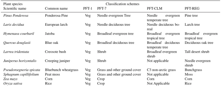
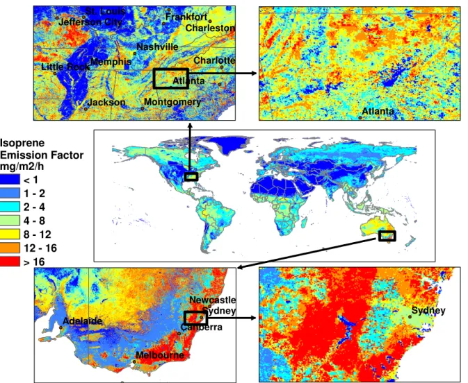
Four different emission factor schemes are illustrated in Tables 1 and 2. The number of vegetation types identified in a scheme ranges from one (PFT-1) to unlimited (PFT-REG). Classification schemes with more categories can be collapsed into those with fewer categories. The PFT-REG scheme is used for regional emission modeling simulations. The stan-dard MEGAN global classification scheme, PFT-7, includes seven PFTs: broadleaf evergreen trees, broadleaf deciduous trees, needle evergreen trees, needle deciduous trees, shrubs, crops, and grass plus other ground cover (e.g., sedges, forbs, and mosses). The PFT-1 scheme, designed for simple sim-ulations, has a single isoprene ε for each location and re-quires considerably less computational resources and fewer driving variables. The global distribution of the MEGAN PFT-1 emission factor is shown in Fig. 2 with a base reso-lution of 30 s (∼1 km). Emission factor hotspots include the southeastern U.S. and southeastern Australia. Figure 2 il-lustrates the considerable variation in ε that occurs on both global and regional (10–100 km) scales. The small scale vari-ability estimated by MEGAN is important for regional mod-eling simulations due to the short lifetime of isoprene and the non-linear chemistry that determines the impact of isoprene on the chemistry of the atmosphere.
Table 3 illustrates how the global average isoprene emis-sion factors differ between and within PFTs. Broadleaf trees and shrubs have the highest average emission factor. The av-erage needle evergreen tree isoprene emission factor is about
Table 1. Description of standard method and available options for calculating MEGAN variables in Eqs. (1) and (2).
Variable Standard method Alternative methods
Emission factor (ε) Use the MEGAN PFT specific ε and PFT
cover databases 1. MEGAN PFT-1 database, with a single ε for each
location.
2. MEGAN PFT-specific ε with user provided PFT cover distributions. This approach can be used for past and future simulations.
3. PFT-REG database which can be extended with user supplied data.
Canopy environment emission activity fac-tor (γCE)
The MEGAN canopy environment model is used to estimate hourly leaf-level PPFD and temperature of sun and shade leaves at each canopy depth as function of PFT type, monthly LAI, hourly tempera-ture, solar radiation (including diffuse and PPFD fractions), wind speed, humidity, and soil moisture. Equations (4–9) are then used to estimate γCE from current and past canopy climate.
1. Solar radiation can be estimated from cloud cover. Diffuse and PPFD fractions can be estimated from solar radiation and sun angle.
2. Hourly weather conditions can be estimated from daily minimum and maximum temperature and daily average values of solar radiation, humidity, wind speed, and soil moisture.
3. MEGAN PFT-1 ε database which requires only one PFT and LAI value for each location. 4. The MEGAN PCEEA algorithm, described by
Eqs. (10) through (15), which requires only LAI, solar transmission, and monthly temperature and PPFD.
Leaf age emission ac-tivity factor (γage)
Estimate with Eqs. (16–19) as a function of current and previous (within the past 7 to 30 days) LAI and average temperature.
1. Assume a constant value (γage=1).
2. Estimate γageas a function of LAI using Eq. (16). 3. Use Eq. (16) with user provided estimates of leaf
age (Fmat, Fnew, Fgro, Fsenin Eq. 16). Soil moisture
emis-sion activity factor (γSM)
Estimate with Eq. (20) as a function of
soil moisture and wilting point 1. Assume a constant value (γSM=1).
2. Use γSM distributions provided on MEGAN data
portal. Canopy loss and
pro-duction (ρISO,ISO)
Estimate with Eq. (21) as a function of canopy depth, friction velocity, and chem-ical lifetime
1. Assume a constant value (ρISO,ISO=0.96).
a factor of six lower than the average broadleaf tree emission factor. The needle deciduous tree and grass PFTs have aver-age emission factors that are about a factor of 20 lower than the average broadleaf tree emission factor, while the crop isoprene emission factor is about two orders of magnitude lower. The substantial differences in these global average isoprene emission factors demonstrates the value of the PFT-7 approach but Table 3 also shows that there is considerable variability associated with the isoprene emission factors as-signed to different species within a single PFT. For example,
the isoprene emission factor for broadleaf trees ranges from 0.1 to 30 mg m−2h−1. Global total isoprene emissions can be approximated using a constant emission factor for each of the seven PFTs but this will introduce significant errors due to correlations between ε and γ distributions. For example, the broadleaf trees that grow in montane and boreal regions often have high isoprene emission factors but low isoprene emission activity factors. Furthermore, there will be sub-stantial errors in estimates for any location where ε deviates significantly from the PFT average ε.
Table 2. Examples of plant species assignments for MEGAN PFT classification schemes.
Plant species Classification schemes
Scientific name Common name PFT-1 PFT-7 PFT-CLM PFT-REG
Pinus Ponderosa Ponderosa Pine Veg Needle evergreen Tree Needle evergreen temperate tree
Pine tree
Larix decidua European larch Veg Needle deciduous tree Needle deciduous bo-real
Larch tree
Hymenaea courbaril Jatoba Veg Broadleaf evergreen tree Broadleaf evergreen tropical tree
Broadleaf evergreen
tropical tree
Quercus douglasii Blue oak Veg Broadleaf deciduous tree Broadleaf deciduous temperate tree
Deciduous oak tree
Larrea tridentata Creosote bush Veg Shrub Broadleaf evergreen
shrub
Tall desert shrub
Juniperus horizontalis Creeping juniper Veg Shrub Not applicable Needle evergreen shrub
Pseudoroegneria spicata Bluebunch wheatgrass Veg Grass and other ground cover C3 non-arctic grass Bunchgrass
Sphagnum capillifolium Peat moss Veg Grass and other ground cover Not applicable Moss
Zea mays Corn Veg Crop Corn Corn
Oryza sativa Rice Veg Crop Not Applicable Rice
Table 3. Global average emission factors, ε (mg isoprene m−2h−1), land area (106km2)and percent contribution to the annual global and regional isoprene emission associated with major plant functional types. The range of land area estimates is based on the PFT databases described in Table 2.
Broadleaf Needle Needle
Evergreen and Evergreen Deciduous Grass
Decid. Trees Trees Trees Shrubs Crops and other
Global ε: Average 12.6 2.0 0.7 10.7 0.09 0.5
Range 0.1 to 30 0.01–13 0.01–2 0.1 to 30 0.01 to 1 0.004 to 1.2
Global land area 13.4 to 38.5 8.6 to 20.0 1.3 to 3.9 15.6 to 24.4 8 to 36.5 17.2 to 38.6
Isoprene Tropical 45% <0.01% <0.01% 28% 0.3% 0.6% Emission Temperate 4.8% 0.3% <0.01% 4.5% <0.01% 0.3% Mediterranean 0.2% 0.1% <0.01% 1.5% <0.01% <0.01% Boreal/Tundra 0.3% 0.4% <0.01% 1.0% <0.01% 0.2% Arid lands 0.3% 0.1% <0.01% 11% <0.01% 0.2% Global 51% 1.1% <0.01% 46% 0.3% 1.4%
Isoprene emission factor distributions for each PFT were estimated by combining the isoprene observations described in Sect. 2 with landcover information that includes ground measurement inventories, satellite based inventories, and ecoregion descriptions. The available landcover and isoprene observations differ considerably for different PFTs and geo-graphic regions. In some cases, vegetation inventories were combined with satellite observations to generate high reso-lution (e.g., 30 m to 1 km) species composition distributions, while in other cases general descriptions were used to char-acterize global ecoregions. A description of these methods is given below.
Since geographical distributions of PFTs and PFT-specific isoprene emission factors change with time, the distributions used to estimate emissions should be representative of the time period being simulated. Climate and land management change can substantially modify species composition and
to-tal vegetation cover, and therefore PFT and ε values, on time scales of weeks to centuries. Emission model investigations of changes in species composition and total vegetation have estimated that significant (10%) isoprene emission changes can occur on a time scale of 25 years for climate driven changes (Martin and Guenther, 1995), 10 years for land management practices such as overgrazing (Guenther et al., 1999b) and two years for land management practices such as cropland abandonment (Schaab et al., 2000). Other land management practices, such as forest clear-cutting, could re-sult in large changes in isoprene emissions over a period of weeks. These studies show that global PFT and ε databases are needed on a time scale of ∼25 years for simulating global earth system changes. A considerably shorter time scale, weeks to a decade, may be required for regional studies in-vestigating the impacts of land cover change.
Jackson Atlanta Memphis Charlotte Nashville Frankfort St. Louis Montgomery Charleston Little Rock Jefferson City Atlanta Sydney Canberra Adelaide Melbourne Newcastle Sydney Isoprene Emission Factor mg/m2/h < 1 1 - 2 2 - 4 4 - 8 8 - 12 12 - 16 > 16
Fig. 2. Global distribution of landscape-average isoprene emission factors (mg isoprene m−2h−1). Spatial variability at the base resolution (∼1 km) is shown by regional images of the southeastern U.S. and southeastern Australia.
3.1.1 Trees
Trees have been the focus of most isoprene emission rate measurement studies and there is a relatively large database for assigning tree emission factors. Trees are also economi-cally valuable which has led to the compilation of high res-olution geographically referenced tree inventories in Eura-sia (e.g., France, Germany, United Kingdom, Japan, China, Russia), North America (e.g., U.S., Canada), Africa (south of the equator), Australia and New Zealand. Biogenic emis-sion inventories have been developed using summaries (i.e., county, province, national totals) based on this information (e.g., Geron et al., 1994; Klinger et al., 2002; Otter et al., 2003; and Simpson et al., 1999). MEGAN integrates plot level species composition data, where available, and regional summaries, for other regions, into the MEGAN PFT-REG database which currently covers all or parts of Eurasia, North America, Australia and New Zealand. The MEGAN PFT-REG distributions and associated species specific emission
factors are used as the basis for weighted average emission factors used with the PFT-CLM, PFT-7, and PFT-1 databases to maintain consistency between regional and global esti-mates.
For regions without quantitative tree inventories, isoprene emission factors are assigned to the 867 ecoregions in the digital terrestrial ecoregion database developed by Olson et al. (2001) and illustrated in Fig. 1. The assigned ε are based on ecoregion descriptions of common plant species and avail-able isoprene emissions measurements. A default value, based on the global average for other regions, is assigned if no measurements are available for characterizing trees in the ecoregion. This scheme provides global coverage using an approach that contains sufficient resolution to simulate biogeographical units with similar isoprene emission char-acteristics. The Olson et al. (2001) database is the product of over 1000 biogeographers, taxonomists, conservation bi-ologists and ecbi-ologists from around the world. Most ecore-gions include a fairly detailed description of the dominant
Broadleaf Trees
Shrubs
Fineleaf Evergreen Trees
Fineleaf Deciduous Trees
Grass and other
Crops < 0.05 0.25 - 0.5 0.5 - 1 1 - 2 2 - 4 4 - 8 8 - 16 Isoprene Emission Factor (mg/m2/h) 0.05-0.25 16 - 33
Fig. 3. Global distribution of isoprene emission factors for the MEGAN PFTs.
plant species found within the region. Uncertainties asso-ciated with ε distributions for tropical broadleaf trees are a major component of the overall uncertainty in global iso-prene emission estimates. Figure 1 shows that there are other large regions, such as boreal forests and tundra forests of Siberia, with no reported observations. All of the dominant tree genera in Siberia have been sampled in other regions but Siberian tree species could have different emission charac-teristics. Accurate emission rates for any region are strongly dependent on the availability of accurate emission rate mea-surements of the regionally dominant species.
Figure 3 illustrates the global distribution of PFT spe-cific isoprene emission factors. Broadleaf tree isoprene emission factors are close to the PFT global average of 12.6 mg m−2h−1in most regions but are <1 mg m−2h−1and ∼20 mg m−2h−1in other regions. Needle evergreen tree ε range from >4 mg m−2h−1 in Canada to <0.5 in the U.S. and Europe. The isoprene emission factors for needle de-ciduous trees are generally very low since this PFT is domi-nated by trees, e.g., larch (Larix), that do not emit substantial amounts of isoprene.
3.1.2 Shrubs, grass and other vegetation
In comparison with trees, there are relatively few measure-ments of isoprene emission factors for shrub, grass, and other plant species. In addition, there is less quantitative data on distributions of these plants due to their lesser eco-nomic importance. However, some countries (e.g., United States, United Kingdom) have landcover characterization ef-forts that include shrubs and ground cover and this informa-tion is being incorporated into the MEGAN emission factors. Shrub emission factors are based on available shrub emis-sion measurements and descriptions of shrub species distri-butions from quantitative ground surveys, in the U.S. only, or estimates based on descriptions of dominant species in each of the 867 Olson ecoregions. The resulting emission fac-tor distribution is illustrated in Fig. 3. The relatively large uncertainty associated with shrub emission factors and the substantial global emission results in a large contribution of shrub isoprene emission to the overall uncertainty in global isoprene emission estimates.
Isoprene emission is rarely observed from plants that are entirely “non-woody”. A rare example is the spider-lily, Hy-menocallis americana (Geron et al., 2006). However, there are a number of isoprene-emitting plants that fall within the MEGAN PFT for grass and other vegetation. Some of the
important isoprene emitting genera in this category include Phragmites (a reed), Carex (a sedge), Stipa (a grass) and Sphagnum (a moss). Reported isoprene emission factors for herbaceous cover range from ∼0.004 mg m−2h−1for grass-lands in Australia (Kirstine et al., 1998) and central U.S. (Fukui and Doskey, 1998) to ∼0.4 mg m−2h−1 for a grass-land in China (Bai et al., 2006) and ∼1.2 mg m−2h−1 for forests and wetlands in southern U.S. (Zimmerman, 1979), northern U.S. (Isebrands et al., 1999), Canada (Klinger et al., 1994) and Scandanavia (Janson et al., 1999). One of these three values is assigned to the grass and other vegetation PFT in each of the 867 ecoregions to develop the emission factor distribution shown in Fig. 3.
3.1.3 Crops
At least one enclosure measurement has characterized each of the 25 globally dominant crop genera and none have been found to emit isoprene (see http://bvoc.acd.ucar.edu). How-ever, agricultural landscapes are isoprene sources in at least some regions. Plantations of isoprene-emitting trees (e.g., poplar, eucalyptus, oil palms) are major isoprene sources at some locations. In addition, isoprene-emitting plants are in-troduced into croplands to increase nitrogen availability and to provide windbreaks. Nitrogen fixing plants grown in crop-lands to provide “green manure” include Velvet bean (Mu-cuna pruriens, a legume) in cornfields and Azolla, an aquatic fern, in rice paddies. Both of these plants produce substantial amounts of isoprene (Silver and Fall, 1995). While the use of Velvet bean is relatively limited, Azolla is widely used in the major rice producing regions (Clark, 1980). Tropical kudzu (Pueraria phaseoloides) is the most widely used “green ma-nure” plant in tropical agricultural lands. Although there are no reported isoprene emission measurements for tropi-cal kudzu, all other examined Pueraria species have been identified as isoprene emitters (e.g., Guenther et al., 1996). We have used the global crop distribution database of Leff et al. (2004) to identify agricultural landscapes (oil palm and rice) where isoprene emissions are likely higher than in other agricultural regions. The elevated isoprene emission associ-ated with oil palm plantations is primarily due to oil palms while rice field isoprene emission is primarily from Azolla, which grows in some but not all rice fields, and not from the rice plants. Additional studies are needed to character-ize the distribution of Azolla in rice fields but presently an isoprene ε of 1 mg m−2h−1is assigned to crop PFT in land-scapes dominated by rice fields. An isoprene emission factor of 10 mg m−2h−1is assigned to crop PFT in areas dominated by oil palm plantations and a value of 0.01 mg m−2h−1is as-signed to all other regions.
3.2 Emission activity factor (γ )
Experimental evidence over the past two decades has impli-cated a number of physical and biological factors in
modify-ing the capacity of a leaf to emit isoprene. Among these fac-tors are incident PPFD and leaf temperature, which control emissions on short (seconds to minutes) time scales (Guen-ther et al., 1993), but which also influence the isoprene emis-sion capacity of a leaf over longer (hours to weeks) time scales (Monson et al., 1994; Sharkey et al., 2000; Geron et al., 2000; Petron et al., 2001). A leaf’s ability to emit isoprene is clearly influenced by leaf phenology; generally speaking, very young leaves of isoprene-emitting species emit no isoprene, mature leaves emit maximally, and as leaves senesce, emission capacity gradually declines. Al-though studies indicate that isoprene emission is less sen-sitive than photosynthesis to decreasing soil moisture (Pego-raro et al., 2004), increasing drought directly effects isoprene emission (as well as indirectly mediating emissions through changes in leaf temperature). Finally, there is growing ev-idence that changes in the composition of the atmosphere, e.g., increased CO2 (Rosenstiel et al., 2003) and episodic increases in ozone (Velikova et al., 2005), may affect iso-prene emission capacity. The available observations of the response of isoprene emission to CO2and O3variations are not suitable for developing robust numerical algorithms and so have not been incorporated into the current version of MEGAN.
The emission activity factor describes variations due to the physiological and phenological processes that drive isoprene emission rate changes. The total emission activity factor is the product of a set of non-dimensional emission activity fac-tors that are each equal to unity at standard conditions,
γ = γCE·γage·γSM (2)
where γCEdescribes variation due to LAI and light, temper-ature, humidity and wind conditions within the canopy envi-ronment, γagemakes adjustments for effects of leaf age, and γSM accounts for direct changes in γ due to changes in soil moisture. Descriptions of the methods used to estimate each of the activity factors included in Eq. (2) are given below. 3.2.1 Canopy environment (γCE)
Isoprene emissions are strongly dependent on leaf tempera-ture and PPFD incident on the leaf (Guenther et al., 1993). Incident PPFD and temperature of leaves within a canopy can differ substantially from above canopy conditions but can be estimated for sun and shade leaves in each layer using a canopy environment model. The canopy average influence of leaf PPFD and temperature, γCE, is estimated as
γCE=CCE·γPT·LAI (3)
where CCE (=0.57 for the MEGAN canopy environment model) is a factor that sets the emission activity to unity at standard conditions, γPT is the weighted average, for all leaves, of the product of a temperature emission activity fac-tor (γT)and a PPFD emission activity factor (γP), and LAI is leaf area index. Note that γP decreases with inceasing LAI.
Leaves in direct sunlight often experience temperatures that are a degree or more higher than ambient air while shaded leaves are often cooler than ambient air temperature. PPFD can be very low on shaded leaves in dense canopies and the PPFD of sun leaves depends on the angle between the sun and the leaf. Guenther et al. (1995) used a rela-tively simple canopy environment model to estimate PPFD on sun and shade leaves at several canopy depths and as-sumed that leaf temperature was equal to air temperature. The non-linear relationships between isoprene emission and environmental conditions, coupled with the strong correla-tion between PPFD and temperature, will result in a sig-nificant underestimation of isoprene emissions if canopy or daily average PPFD and temperature are used (rather than calculating emissions for each canopy level and each hour of the day). Lamb et al. (1996) evaluated the use of several canopy environment models for predicting whole canopy iso-prene fluxes and found that the results from both simple and complex canopy models were within the uncertainty range of observed isoprene fluxes. Although detailed canopy envi-ronment models may not always substantially improve iso-prene emission estimates, these models may be important for investigating how changes in environmental conditions will perturb isoprene emission rates. The integration of MEGAN within the land surface model component of an earth system model will allow investigations of interactions between iso-prene emissions and environmental conditions. The standard MEGAN canopy environment model is based on the methods described by Guenther et al. (1999a). This model estimates incident PPFD and temperature of sun and shade leaves at five canopy depths. It includes a leaf energy balance model that is driven by wind speed, humidity, solar insolation, am-bient temperature, and soil moisture. The model also calcu-lates whole canopy latent and sensible heat fluxes that can be evaluated by above canopy measurements. Other canopy environment models can be used with MEGAN by setting CCEso that γCEis equal to unity for the MEGAN standard conditions.
The algorithms described by Guenther et al. (1993) and modified by Guenther et al. (1999a) have been used ex-tensively to simulate the response of isoprene emission to changes in light and temperature on a time scale of seconds to minutes. The Guenther et al. (1999a) algorithms simulate emission variations as
γP=CP[(α ·PPFD)/((1 + α2·PPFD2)0.5)] (4) γT=Eopt· [CT2·exp(CT1·x)/(CT2−CT1·(1− exp(CT2·x)))](5)
where PPFD is the leaf level photosynthetic photon flux den-sity (µmol m−2s−1), x=[(1/Topt)–(1/T)]/0.00831, T is leaf temperature (K), CT1 (=95), CT2 (=230), CP ,α, Eopt, and Topt are empirical coefficients. MEGAN extends this al-gorithm by estimating CP ,α,Eopt, and Topt using Eqs. (6) through (9) instead of using the constant values recom-mended by Guenther et al. (1999a). The main advantage of
this approach is improved simulations of the variations in iso-prene emission associated with past temperature and PPFD conditions. The light and temperature conditions of the past day(s) result in substantial deviations from the Guenther et al. (1993) algorithms that could be due to changes in produc-tion of the isoprene substrate, dimethylallyl pyrophosphate (DMAPP), and/or variations in the activity of isoprene syn-thase (Fall and Wildermuth, 1998), the enzyme that converts DMAPP to isoprene. Variations in DMAPP supply could be due to changes in production, either availability of the carbon precursor (pyruvate) or adenosine triphosphate (ATP) used for phosphorylation, or changes in DMAPP consump-tion. Variations in isoprene synthase activity and DMAPP have been observed but are not well characterized (Brugge-mann et al., 2002; Wolfertz et al., 2003). Isoprene emis-sion rates, measured at standard light and temperature condi-tions, are higher when warm sunny conditions have occurred during the previous day(s) and are lower if there were cool shady conditions (Sharkey et al., 2000). Petron et al. (2001) found that exposure to high or low temperatures can influ-ence isoprene emission for several weeks. The time required to reach a new, lower, steady-state isoprene emission capac-ity following a step decrease in temperature was longer than that required to reach a new, higher, equilibrium following an increase in temperature, indicating that down regulation of isoprene emission is a slower process than up regulation. The factors controlling these variations may operate over a continuous range of time scales, but for modeling purposes MEGAN currently considers only 24 and 240 h. The average leaf level PPFD of the past 24 h (P24)and past 240 h (P240) influence the estimated emission activity by adjusting the co-efficients in Eq. (4) as follows,
α =0.004 − 0.0005 ln(P240) (6) CP =0.0468 · exp(0.0005 · [P24−P0]) · [P240]0.6 (7) where P0 is equal to 200 µmol m−2s−1 for sun leaves and 50 µmol m−2s−1for shade leaves.
MEGAN estimates the coefficients in Eq. (5) as a function of the average leaf temperature over the past 24 (T24)and 240 (T240)h, as follows,
Topt=313 + (0.6 · (T240−297)) (8) Eopt=2.034·exp(0.05·(T24−297))·exp(0.05·(T240−297)).(9) The coefficients used for Eqs. (6–9) are based on observa-tions reported by Petron et al. (2001), Monson et al. (1994), Sharkey et al. (2000), Geron et al. (2000), and Hanson and Sharkey (2001). Although these five studies report results that are qualitatively similar, there remain significant uncer-tainties associated with these algorithms.
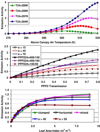
Figure 4 shows the response of γCEestimates to variations in LAI, solar angle and transmission, and temperature. Iso-prene emission increases exponentially with temperature up
to a maximum that is dependent on the average temperature that the canopy has experienced during the past 240 h. Both the magnitude of the emissions and the temperature at which the maximum occurs are dependent on the past temperature. The result is that MEGAN predicts lower (higher) isoprene emissions in cool (warm) climates than would be simulated by the Guenther et al. (1993) algorithms. However, MEGAN predictions of the isoprene emission response to short term (<24 h) temperature variations is often less than that pre-dicted by models that do not calculate leaf temperature, e.g., BEIS2/BEIS3 or Guenther et al. (1995). This is because leaf transpiration tends to result in leaf temperature increases that are less than ambient temperature increases.
Above canopy PPFD is determined by solar angle and transmission. MEGAN estimates of γCE increase nearly linearly with PPFD transmission for canopies that have experienced high PPFD levels (e.g., 24 h average of 600 µmol m−2s−1for sun leaves) during the past day. The emission increase begins to saturate at high PPFD transmis-sion for low solar angles or if the average PPFD has been low during the previous day.
Figure 4 shows that estimated isoprene emission increases nearly linearly with LAI until LAI exceeds ∼1.5 and is nearly constant for LAI>5. The relationship between LAI and γCE depends on solar angle and on canopy charac-teristics, which differ with PFT. Isoprene emissions from canopies with clumped leaves increase relatively slowly with increasing LAI for LAI<3 in contrast to canopies with horizontal leaves that exhibit a stronger LAI dependence for LAI<3. Figure 4 also shows that MEGAN predicts a stronger initial increase with LAI, and a lack of increase with higher LAI, for low solar angles (e.g., <30 degrees).
As an alternative to using a detailed canopy environment model that calculates light and temperature at each canopy depth, we have developed a parameterized approach, referred to here as the parameterized canopy environment emission activity (PCEEA) algorithm, based on the results of the pro-cedures described above. The PCEEA approach for estimat-ing the canopy environment emission activity factor is as fol-lows,
γCE=γLAI·γP ·γT (10)
where γLAI, γP and γT account for variations associated with LAI, PPFD and temperature. The relationships be-tween these factors and canopy scale isoprene emissions are based on MEGAN canopy environment model simulations for the canopies and environmental conditions that dominate global isoprene emissions (i.e., warm broadleaf forests). The canopy-scale isoprene emission response to PPFD variations is simulated as γP =0 a <0, a > 180 (11a) γP =sin(a)[2.46(1 + 0.0005 · (Pdaily−400))φ · 0.9φ2] 0 < a < 180 (11b) 0 0.2 0.4 0.6 0.8 1 1.2 1.4 0 2.5 5 7.5 10
Leaf Area Index (m2 m-2)
Em is si on A ct iv ity
clumped horizontal mixed a = 40 a = 20 0 1 2 3 4 270 280 290 300 310 320
Above Canopy Air Temperature (K)
Em is si on A ct iv ity T24=280KT24=290K T24=297K T24=304K 0 0.5 1 1.5 2 2.5 0 0.1 0.2 0.3 0.4 0.5 0.6 0.7 0.8 PPFD Transmission Em is si on A ct iv ity a = 15 a = 45 a = 70 PPFD24=600/150 PPFD24=400/100 PPFD24=100/50 0 0.2 0.4 0.6 0.8 1 1.2 1.4 0 2.5 5 7.5 10
Leaf Area Index (m2 m-2)
Em is si on A ct iv ity
clumped horizontal mixed a = 40 a = 20 0 1 2 3 270 280 290 300 310 320
Above Canopy Air Temperature (K)
Em is si on A ct iv ity T24=280KT24=290K T24=297K T24=304K 0 0.5 1 1.5 2 2.5 0 0.1 0.2 0.3 0.4 0.5 0.6 0.7 0.8 PPFD Transmission Em is si on A ct iv ity a = 15 a = 45 a = 70 PPFD24=600/150 PPFD24=400/100 PPFD24=100/50
Fig. 4. MEGAN estimates of isoprene emission response to current temperature (top), PPFD transmission (middle) and LAI (bottom). The response to current temperature is estimated for leaves exposed to different average temperatures (280 K, 290 K, 297 K and 305 K) during the past 24 to 240 h (T24=T240in each case). The response to current PPFD transmission is estimated for leaves exposed to dif-ferent solar angles (15, 45 and 70 degrees) and for average PPFD levels for the past 24 to 240 h (PPFD24=PPFD240in each case) that include 600 and 150 µmol m−2s−1, respectively, for sun leaves and shade leaves, 400 and 100 µmol m−2s−1for sun and shade leaves, and 100 and 50 µmol m−2s−1for sun and shade leaves. The re-sponse to LAI (for a constant PPFD transmission of 60%) is es-timated for different canopy leaf orientations (clumped, horizontal and mixed leaves with a solar angle of 60 degrees) and solar angles (20 and 40 degrees with a mixed leaf orientation).
where Pdaily is daily average above canopy PPFD (µmol m−2s−1)representative of the simulation period (typ-ically a week to a month), a is solar angle (degrees) and φ is above canopy PPFD transmission (non-dimensional) which is estimated as
φ = Pac/(sin(a)Ptoa) (12)
where Pac is above canopy PPFD, Ptoa is PPFD (µmol m−2s−1)at the top of the atmosphere which can be approximated as
Ptoa=3000 + 99 · cos(2 · 3.14 · (DOY − 10)/365) (13) where DOY is day of year.
The temperature response factor, γT, is estimated as γT=Eopt·CT2·exp(CT1·x)/(CT2−CT1·(1− exp(CT2·x))) (14)
where x=[(1/Topt)–(1/Thr)]/0.00831, Eopt=1.75·exp(0.08 (Tdaily–297)), Thr is hourly average air temperature (K), Tdailyis daily average air temperature (K) representative of the simulation period (typically a week to a month), CT1 (=80), CT2(=200), are empirical coefficients and Toptis es-timated using Eq. (8) with Tdailyused in place of T240. Emis-sion responses to LAI variations are estimated as
γLAI=0.49LAI/[(1 + 0.2LAI2)0.5]. (15) The PCEEA approach is intended for applications that need to minimize the computational resources or have limited availability of driving variables. The PCEEA algorithm esti-mates annual global isoprene emissions that are within ∼5% of the value estimated using the standard MEGAN canopy environment model. However, differences can exceed 25% for estimates at specific times and locations.
3.2.2 Leaf age
Leaves begin to photosynthesize soon after budbreak but iso-prene is not emitted in substantial quantities for days after the onset of photosynthesis (Guenther et al., 1991). In ad-dition, old leaves eventually lose their ability to photosyn-thesize and produce isoprene. Guenther et al. (1999a) devel-oped a simple algorithm to simulate the reduced emissions expected for young and old leaves based on the observed monthly LAI change. An increase in foliage was assumed to imply a higher proportion of young leaves while decreas-ing foliage was associated with the presence of older leaves. This algorithm required a time step of one month, assumed that young leaves and old leaves had the same emission rate, and included variables that could not easily be quantified. The following procedures to account for leaf age effects on isoprene emission estimates reduce these deficiencies.
MEGAN assumes a constant value, γage=1, for evergreen canopies. Deciduous canopies are divided into four fractions: new foliage that emits negligible amounts of isoprene (Fnew), growing foliage that emits isoprene at less than peak rates (Fgro), mature foliage that emits isoprene at peak rates (Fmat) and old foliage that emits isoprene at reduced rates (Fold). The canopy-weighted average factor is calculated as γage=FnewAnew+FgroAgro+FmatAmat+FoldAold (16) where Anew (=0.05), Agro (=0.6), Amat (=1.125), and Aold (=1) are the relative emission rates assigned to each canopy fraction. The values of these emission factors are based on the observations of Petron et al. (2001), Goldstein et al. (1998), Monson et al. (1994), Guenther et al. (1991) and Karl et al. (2003).
The canopy is divided into leaf age fractions based on the change in LAI between the current time step (LAIc)and the
previous time step (LAIp). In cases where LAIc=LAIp then Fmat=0.8, Fnew=0, Fgro=0.1, Fold=0.1. When LAIp>LAIc then Fnew and Fgro are equal to zero, Fold is estimated as [(LAIp–LAIc)/LAIp] and Fmat=1–Fold. In the final case, where LAIp<LAIc, Fold=0 and the other fractions are cal-culated as
Fnew=1 − (LAIp/LAIc)for t <= ti (17a) Fnew= [ti/t ][1 − (LAIp/LAIc)]for t > ti (17b) Fmat=(LAIp/LAIc)for t <= tm (17c) Fmat=(LAIp/LAIc)+[(t −tm)/t ][1−(LAIp/LAIc)]for t >tm (17d)
Fgro=1 − Fnew−Fmat (17e)
where t is the length of the time step (days) between LAIc and LAIp, tiis the number of days between budbreak and the induction of isoprene emission, tmis the number of days be-tween budbreak and the initiation of peak isoprene emission rates, and tg=tmfor t >tmand tg=tfor t≤tm. The time step, t, depends on the LAI database that is used but generally is between one week and one month. Petron et al. (2001) grew plants under conditions typical of temperate regions and ob-served an emission pattern that suggests a tiof about 12 days and tmof about 28 days. Goldstein et al. (1998) field obser-vations in a temperate forest indicate a similar value for tm. Monson et al. (1994) found that tiand tmare temperature de-pendent and are considerably less for vegetation growing at high temperatures. These observations suggest that the tem-perature dependence of these variables can be estimated as ti =5 + (0.7 · (300 − Tt))for ti ≤303 (18a) ti =2.9 for ti >303 (18b)
tm=2.3 · ti (19)
where Tt is the average ambient air temperature (K) of the preceding time step interval. MEGAN simulations using a constant ti and tm result in global annual isoprene emis-sions that are ∼5% lower than estimates based on a variable ti. However, the emission rates estimated using variable ti and tm can be as much as 20% higher in tropical regions and 20% lower in boreal regions when foliage is rapidly ex-panding. The differences are more pronounced when LAI variations have a higher time resolution (i.e., weekly rather than monthly). Equations (18) and (19) are important for higher resolution simulations and when foliage is expanding but otherwise have only a minimal impact on estimated emis-sions.
3.2.3 Soil moisture
Plants require both carbon dioxide and water for growth. Carbon dioxide is taken up through leaf stomatal openings and water is usually obtained from the soil. However, large quantities of water are lost through stomata creating a need
for adequate soil moisture in order to continue carbon up-take. Field measurements have shown that plants with inad-equate soil moisture can have significantly decreased stom-atal conductance and photosynthesis, in comparison to well-watered plants, and yet can maintain approximately the same isoprene emission rates (Guenther et al., 1999b). However, isoprene emission does begin to decrease when soil moisture drops below a certain level and eventually becomes negligi-ble when plants are exposed to extended severe drought (Pe-goraro et al., 2004). MEGAN can simulate the response of isoprene emission to drought through two mechanisms. Iso-prene emissions are indirectly influenced by the soil mois-ture dependence of stomatal conductance which influences the leaf temperature estimated by the MEGAN canopy envi-ronment model. In addition, MEGAN includes an emission activity factor, dependent on soil moisture, estimated as
γSM =1 θ > θ1 (20a)
γSM =(θ − θw)/1θ1 θw< θ < θ1 (20b)
γSM =0 θ < θw (20c)
where θ is soil moisture (volumetric water content, m3m−3), θw (m3m−3)is wilting point (the soil moisture level below which plants cannot extract water from soil) and 1θ1(=0.06) is an empirical parameter based on the observations of Pe-goraro et al. (2004), and θ1=θw+1θ1. MEGAN uses the high resolution (∼1 km2)wilting point database developed by Chen and Dudhia (2001) which assigns θw values that range from 0.01 for sand to 0.138 m3m−3for clay soils. Soil moisture varies significantly with depth and the ability of a plant to extract water is dependent on root depth. MEGAN uses the PFT dependent approach described by Zeng (2001) to determine the fraction of roots within each soil layer and applies the weighted average γSM for each soil layer. This approach allows soil moisture estimates from any soil depth to be used in Eq. (20).
Including the influence of soil moisture on isoprene emis-sion (Eq. 20) reduces annual global isoprene emisemis-sions by only ∼7% but can reduce regional emissions to zero for days to months. As expected, the soil moisture emission activ-ity factor has the greatest impact on isoprene emissions es-timated for arid regions. However, significant reductions in estimated emissions also occur in regions that have moderate to high total annual precipitation but also have dry seasons with little rainfall.
3.2.4 Other factors that influence isoprene emission activ-ity
Isoprene emission activity can also be influenced by other environmental conditions including ozone (Velikova et al., 2005) and carbon dioxide (Buckley, 2001; Rosenstiel et al., 2003) concentrations, nitrogen availability (Harley et al., 1994), and physical stress (e.g., Alessio et al., 2004). In ad-dition, there may be significant diurnal variations that are not
entirely explained by variations in environmental conditions (Funk et al., 2003). Emission activity factors accounting for these processes will be included in MEGAN as more reliable algorithms are developed. Existing observations have been used to qualitatively assess the importance of these factors and are discussed in Sect. 6.
3.3 Canopy loss and production, ρ
Chemicals emitted into the canopy airspace do not always escape to the above-canopy atmosphere. Some molecules are consumed by biological, chemical and physical processes on soil and vegetation surfaces while others react within the canopy atmosphere. Some emissions escape to the above-canopy atmosphere in a different chemical and/or physi-cal (i.e., gas to particle conversion) form. MEGAN in-cludes a factor, ρ, that accounts for losses and transforma-tions in the canopy. The resulting emission estimate is a net canopy emission but is not the net flux. The net ecosystem-atmosphere isoprene flux is the sum of the MEGAN net emission rate estimate and an above-canopy deposition rate that can be estimated from an above-canopy concentration and a deposition velocity. The MEGAN canopy loss factor for isoprene, ρISO,ISO, is the ratio of isoprene emitted into the above canopy atmosphere to the isoprene emitted into the canopy atmosphere. Additional factors account for the emission of gases and aerosols produced from the oxidation of isoprene within the canopy. For example, the MEGAN canopy production factor for the isoprene oxidation prod-uct formaldehyde, ρCH2O,ISO, is the ratio of formaldehyde (produced from isoprene oxidation) emitted into the above canopy atmosphere to the isoprene emitted into the canopy atmosphere.
Inverse modeling of within-canopy gradients of isoprene suggests that at least 90% of the isoprene emitted by tropi-cal and temperate forests escapes to the above-canopy atmo-sphere (Karl et al., 2004; Stroud et al., 2005). The remainder is removed through a combination of chemical losses and dry deposition. While ambient mixing ratios within the canopy and roughness layer can change on the order of 10–30% due to chemistry (Makar et al., 1999), the bias of canopy scale isoprene flux measurements is small (i.e., on the order of 5– 10%). This can be attributed to (1) near field effects within the canopy and (2) limited processing time between the loca-tion of isoprene emission (occurring mostly within the upper canopy) and the top of the canopy. Comparisons between canopy-scale emissions based on leaf-level emission mea-surements extrapolated with a canopy environment model and above-canopy flux measurements tend to show that any loss of isoprene is less than the uncertainty associated with these two approaches (Guenther et al., 1996; Guenther et al., 2000; Spirig et al., 2005).
Variations in isoprene canopy production and loss are es-timated as
where D is canopy depth (m), u* is friction velocity (m s−1), τ is the above-canopy isoprene lifetime (s) and λ is an em-pirically determined parameter. Canopy depth is the distance from the top to the bottom of the canopy and can be consid-erable less than canopy height. Equation (21) is parameter-ized with the above-canopy isoprene lifetime, rather than the within-canopy lifetime, because this is the value more read-ily available for atmospheric modeling. D and λ are PFT dependent and are assigned D=15 and λ=0.3 for the generic PFT-1 canopy. Since values of ρISO,ISO range only from 0.93 to 0.99 for most conditions, Table 1 includes assign-ing a constant value, ρISO,ISO=0.96 for isoprene emission estimation efforts. The variability is greater for more reac-tive compounds such as the sesquiterpene, β-caryophyllene, for which the canopy loss factor ρCARY,CARY can vary from <0.1 to >0.6 depending on environmental conditions. Equa-tion (21) is based on measured isoprene emission profiles and turbulence profiles obtained during recent tropical and temperate forest field studies (Karl et al., 2004; Stroud et al., 2005). The variation of the isoprene lifetime inside the canopy was scaled to the above-canopy lifetime and based on measured O3profiles and modeled OH and NO3 levels reported by Stroud et al. (2005). A random walk model sim-ilar to the one described by Baldocchi (1997) and Strong et al. (2004) was used to estimate the first order decay of iso-prene. Trajectories for 5000 particles were released at 4 lev-els and computed for typical daytime conditions. The chem-ical loss by the ensemble mean was used to assess ρISO,ISO integrated over the whole canopy.
Model simulations of the impact of isoprene on at-mospheric chemistry depend on estimates of net isoprene emission as well as estimates of the regional uptake of isoprene and its oxidation products, e.g. methylvinylke-tone, methacrolein and peroxyacetyl nitrate (PAN), from the above-canopy atmosphere. Karl et al. (2004) conclude that current model procedures can underestimate the uptake of these oxidation products which would cause an overestimate of the impact of isoprene on oxidants and other atmospheric constituents. They also report that isoprene oxidation prod-ucts deposit more rapidly during night than predicted by stan-dard dry deposition schemes. During daytime, the net effect of deposition and in-canopy production of these compounds can be on the same order. These observations raise the pos-sibility that various products of isoprene chemistry are taken up by the forest canopy more efficiently then previously as-sumed. This could lead to an incorrect characterization of the impact of isoprene by chemistry and transport models that have correctly simulated isoprene emission rates and ox-idation schemes, and could explain why some chemistry and transport models are forced to use isoprene emission rates that are lower than observed.
4 Driving variables
The MEGAN algorithms described in Sect. 3 require esti-mates of landcover (LAI and PFT distributions) and weather (solar transmission, air temperature, humidity, wind speed, and soil moisture) conditions. The standard driving variables used for MEGAN are described in this section and are com-pared with alternative databases.
4.1 Leaf area
MEGAN requires leaf area estimates with a time step of ∼4 to 40 days in order to simulate seasonal variations in leaf biomass and age distribution. MEGAN does not assume that LAI is uniformly spread over a grid cell but assumes that foliage covers only that part of the grid cell containing veg-etation. The average LAI for vegetated areas is estimated by dividing the grid average LAI by the fraction of the grid that is covered by vegetation. We refer to this as LAIv (the LAI of vegetation covered surfaces) and we set an upper limit of LAIv=6 to eliminate the very high values that can be estimated for grids with very little vegetation. The stan-dard MEGAN LAIv database (MEGAN-L) was estimated by this approach using the LAI estimates of Zhang et al. (2004) and estimates of vegetation cover fraction from Hansen et al. (2003). These data were processed to include values for missing data and urban areas.
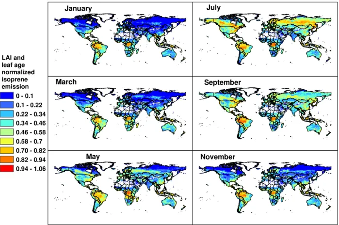
Figure 5 illustrates how LAIv variations with time and lo-cation result in isoprene emission variations of more than an order of magnitude, independent of variation in other driv-ing variables which are held constant in these simulations. These emission variations are driven by changes in only leaf age and quantity. Isoprene is reduced by more than a factor of five at higher latitudes in winter but varies only ∼15% for croplands, forests and grasslands during the growing season. Most of the extra-tropical regions of the southern hemisphere do not exceed a level of 30% of the maximum emission while tropical forests regions rarely fall below a level of 70%.
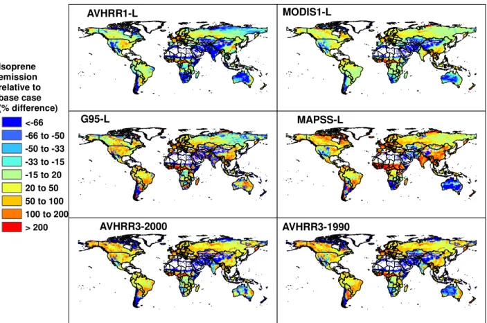
Table 4 includes descriptions of six LAI databases that have been used to estimate global isoprene emissions with MEGAN. Satellite-derived LAI estimates provide high res-olution variability but are not available for all years. Dy-namic vegetation models allow predictions of past and fu-ture emissions. The MEGAN-L database contains monthly estimates for years 2000 to 2005 at 30 s (∼1 km2) resolu-tion. Table 4 includes a comparison of annual global isoprene emissions estimated with alternative LAIv databases. The estimates range from 11% lower to 29% higher than the MEGAN-L values. Some of the differences are due to in-terannual variations, which can be seen in Fig. 6 by the com-parison of July average isoprene emissions estimated with the AVHRR3 databases for years 1990 and 2000. The emis-sion estimates using MODIS based estimates of LAI, includ-ing the MEGAN-L database, are generally ∼20% lower than emission estimates using the other LAI databases. All of the
January March May July September November LAI and leaf age normalized isoprene emission 0 - 0.1 0.1 - 0.22 0.22 - 0.34 0.34 - 0.46 0.46 - 0.58 0.58 - 0.7 0.70 - 0.82 0.82 - 0.94 0.94 - 1.06
Fig. 5. Monthly normalized isoprene emission rates estimated with MEGAN for 2003. Rates are normalized by the emission estimated for standard LAI (=5 m2m−2)and leaf age (80% mature leaves). These normalized rates illustrate the variations associated with changes in only LAI and leaf age; i.e. all other model drivers are held constant.
databases shown in Fig. 6 have regions of more than a fac-tor of 3 lower emissions and regions with more than a facfac-tor of 3 higher emissions. However, the regions with the great-est percent differences tend to be areas with relatively low emissions.
4.2 PFT distributions
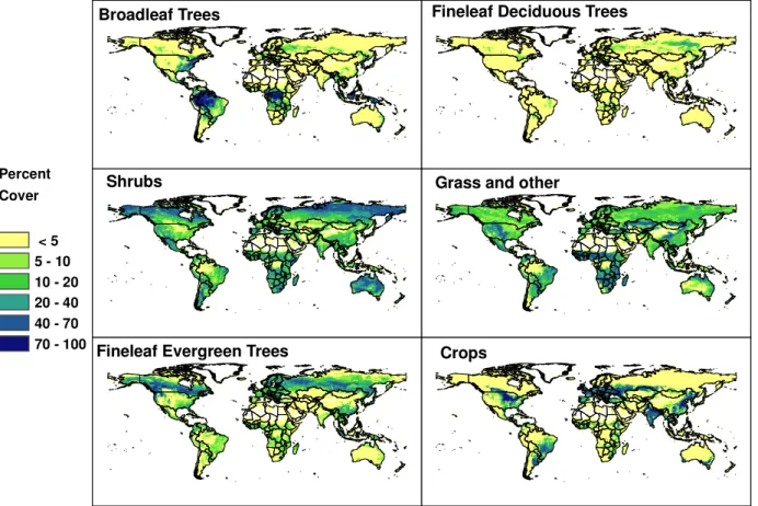
The PFT databases described in Table 4 use a variety of in-puts including satellite observations, vegetation inventories, ecosystem maps, and ecosystem model output. The satellite data provide the highest spatial and temporal resolution while only models can be used to simulate future scenarios. Vege-tation inventories based on field observations are expected to provide the most accurate estimates of PFT distributions but they have limited coverage.
Landcover data were processed to generate the MEGAN PFT categories from each data source shown in Table 4. Landcover data that included PFT estimates (AVHRR1-P, MODIS1-P), were converted into the MEGAN PFT scheme with a straightforward collapsing of their fifteen PFTs into the seven MEGAN PFTs. The ecosystem scheme databases (HYDE, GED, IBIS, IMAGE, MODIS2, SPOT) contain a
discrete landcover type for each location that is based on ei-ther observed vegetation distribution maps, vegetation model output or satellite observations. A PFT distribution was as-sumed for each ecosystem type in each database. For ex-ample, the temperate mixed forest ecosystem in the GED database was assumed to be composed of 20% broadleaf deciduous trees, 20% broadleaf evergreen trees, 40% nee-dle evergreen trees, 1% neenee-dle deciduous trees, 1% shrubs, 1% crops, 2% herbaceous and 15% bare ground or water. These subjective PFT assignments were based on qualita-tive descriptions of the ecosystems. The IMAGE database includes estimates for years 2000 and 2100 and the HYDE database has estimates for 50 year intervals between 1700 and 1950 and 20 year intervals between 1950 and 1990. The AVHRR2 and MODIS3 databases use satellite derived tree cover data that include total cover, and deciduous and broadleaf fractions. These provide the most direct estimates for the MEGAN tree PFTs and constrain the total fraction assigned to the other three MEGAN PFTs. The standard MEGAN PFT database (MEGAN-P) combines the MODIS3 database with quantitative tree inventories based on ground observations where available (e.g., Kinnee et al., 1997). The global distribution of each PFT in the MEGAN database is