Conic Optimization of Electric Power Systems
by
Joshua Adam Taylor
B.S.,
Carnegie Mellon University (2006)
S.M., Massachusetts Institute of Technology (2008)
Submitted to the Department of Mechanical Engineering
MASSACHUSETTS INSTITUTE OF TECHNOLOGY
JUL 29 2011
LIBRARIES
ARCHN'ES
in partial fulfillment of the requirements for the degree of
Doctor of Philosophy
at the
MASSACHUSETTS INSTITUTE OF TECHNOLOGY
June 2011
©
Massachusetts Institute of Technology 2011. All rights reserved.
A uthor ...
...
...
..
...
Department of Mechanical Engineering
June 2, 2011
Certified by...
Finmeccanica Career
Franz S. Hover
Development Professor of Engineering
Thesis Supervisor
Accepted by ... .. ...
David E. Hardt
Chairman, Department Committee on Graduate Students
Conic Optimization of Electric Power Systems
by
Joshua Adam Taylor
Submitted to the Department of Mechanical Engineering on May 1, 2011, in partial fulfillment of the
requirements for the degree of Doctor of Philosophy
Abstract
The electric power grid is recognized as an essential modern infrastructure that poses numerous canonical design and operational problems. Perhaps most critically, the inherently large scale of the power grid and similar systems necessitates fast algo-rithms. A particular complication distinguishing problems in power systems from those arising in other large infrastructures is the mathematical description of alter-nating current power flow: it is nonconvex, and thus excludes power systems from many frameworks benefiting from theoretically and practically efficient algorithms. However, advances over the past twenty years in optimization have led to broader classes possessing such algorithms, as well as procedures for transferring nonconvex problem to these classes.
In this thesis, we approximate difficult problems in power systems with tractable, conic programs. First, we formulate a new type of NP-hard graph cut arising from undirected multicommodity flow networks. An eigenvalue bound in the form of the Cheeger inequality is proven, which serves as a starting point for deriving semidefinite relaxations. We next apply a lift-and-project type relaxation to transmission system planning. The approach unifies and improves upon existing models based on the DC power flow approximation, and yields new mixed-integer linear, second-order cone, and semidefinite models for the AC case. The AC models are particularly applicable to scenarios in which the DC approximation is not justified, such as the all-electric ship. Lastly, we consider distribution system reconfiguration. By making physi-cally motivated simplifications to the DistFlow equations, we obtain mixed-integer quadratic, quadratically constrained, and second-order cone formulations, which are accurate and efficient enough for near-optimal, real-time application.
We test each model on standard benchmark problems, as well as a new bench-mark abstracted from a notional shipboard power system. The models accurately approximate the original formulations, while demonstrating the scalability required for application to realistic systems. Collectively, the models provide tangible new tradeoffs between computational efficiency and accuracy for fundamental problems in power systems.
Thesis Supervisor: Franz S. Hover
Acknowledgments
As a student in the ocean area of a mechanical engineering department working on terrestrial power systems, it was tempting to make the title of this thesis something like 'fighting the current' or 'against the flow'; yet, I could not have imagined a better course to have taken through graduate school, and this is largely due to the people who accompanied me along the way. First, an enormous thanks to my advisor, Professor Franz Hover, who taught me (among many things) never fear to apply my own creativity, and who has also become a close friend.
I'd like to thank my committee, Professors Jim Kirtley, Sanjay Sarma, and John Tsitsiklis for their thoughtful guidance and advice over the past two years. A large portion of Chapter 3 benefited from discussions with Professor Daniel Stroock when I was stuck. Dr. Julie Chalfant deserves special thanks for helping me formulate the example in Section 4.6.4.
Over the past five years, I've been privileged to wonderful friends, without whom this experience would not have been what it was. As a member of the Hovergroup, I've had the pleasure of daily interaction with a number of smart and interesting people, all of whom I'd like to acknowledge, but especially Matt Greytak and Brendan Englot; I hope that we can continue our conversations in the future, if perhaps from different fields. The game of squash has been an essential outlet for me, and it will be difficult if not impossible to find substitutes for my weekly matches with Woradorn Wattanapanitch and Arup Chakraborty, as well as the rest of the MIT squash community. I feel truly lucky to have been been through some unforgettably fun times with a very cohesive circle of friends: my two amigos, Austin Minnich and Allison Beese, Matthew Branham, Eerik Hantsoo, Priam Pillai, Erica Ueda, and Kit Werley. And, because he requested it, but also because he's been my best friend for many years, Daniel Muenz gets mentioned now.
Every year I realize more and more what an incredible family I have, and how much they have shaped who I am. Stuart and Sheila, Rachel and David: this thesis is dedicated to you.
Support is acknowledged from the Office of Naval Research, Grant N00014-02-1-0623.
Contents
1 Introduction
1.1 Motivation.. . . . ...
1.2 Overview and contributions... . . ...
2 Background
2.1 Steady state power flow . . . . 2.2 Conic optimization . ...
2.3 Lift-and-project relaxations ...
2.4 Literature review . . . . 2.4.1 Spectral graph theory and multicommodity flow netw 2.4.2 Transmission system planning ...
2.4.3 Distribution system reconfiguration . . . . ... 2.5 General perspective... . . . . . .
3 Spectral graph theory and multicommodity flow networks 3.1 Introduction... . . . . ..
3.2 Background.. . . . . . ...
3.2.1 The Laplacian of a graph and the Cheeger constant . 3.2.2 Flow networks . . . . 3.3 A flow-based Cheeger constant . . . . 3.4 Laplacians for flow networks.... . . . . ..
3.4.1 Variational formulation . . . ... 3.4.2 Bounds on p . . . . )rks 19 . . . 21 . . . 22 . . . 25 . . . 25 . . . 26 27 27
3.4.3 Orthogonality constraints . . . . 40
3.4.4 Calculation via orthogonal transformation... . . . .. 43
3.5 An alternate relaxation of q... . . . . . . . . 44
3.6 Semidefinite programming with many commodities . . . . 45
3.6.1 Relaxing pr . . . ..46
3.6.2 R elaxing -y . . . . 48
3.7 Computational results... . . . . . . .. 49
3.7.1 One commodity... . . . . . . . .. 49
3.7.2 Multiple commodities.. . . . . . . . . 50
3.8 Application: Stochastic flow networks.. . . . . . . . . . 51
3.8.1 Bounds using Weyl's theorem . . . . 52
3.8.2 Approximation using perturbation theory... . . . . .. 54
3.9 Sum m ary . . . . 57
4 Transmission system planning 59 4.1 Introduction... . . . . . . . . . .. 59 4.2 DC power flow... . . . . . . . 60 4.2.1 Network design . . . . 60 4.2.2 Linear m odels . . . . 61 4.3 AC power flow... . . . . . . . . 63 4.3.1 Linear m odels . . . . 64
4.3.2 Semidefinite and second-order cone models . . . . 68
4.4 Related problems of interest . . . . 70
4.4.1 Direct current systems . . . . 71
4.4.2 M ultiple scenarios . . . . 71
4.5 Design fram ework . . . . 72
4.6 Computational results... . . . . . . . . .. 73
4.6.1 D C m odels . . . . 74
4.6.2 Linear AC models . . . . 74
4.6.3 Nonlinear AC models . . . . 79 8
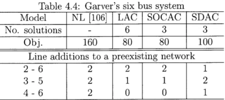
4.6.4 Shipboard power system . . . . . 4.6.5 Interpretation of results . . . . . 4.7 Sum m ary . . . .
5 Distribution system reconfiguration 5.1 Introduction.... . . . . . ... 5.2 The DistFlow equations.... . . ...
5.3 Quadratic programming . . . . 5.4 Quadratically constrained programming . ...
5.5 Second-order cone programming ... 5.6 Computational examples . . . . ...
5.7 Sum m ary . . . .
List of Figures
2-1 Relationships between chapters... . . . . . . . ... 28
3-1 Graph bottlenecking as measured by h (left) versus flow bottlenecking as m easured by q (right) . . . . 34 3-2 IEEE 118 bus test system feasibility pdf's. Increasing along the 'i-axis
implies 'higher' feasibility... . . . . . . . ... 56
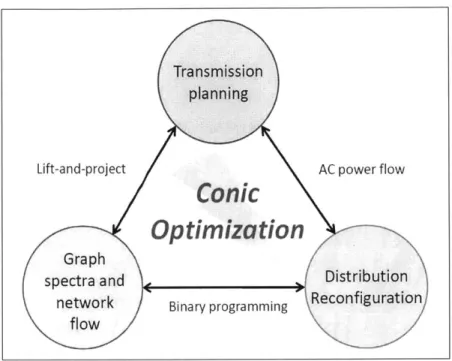
4-1 46-bus Brazilian system (from [68]). Dashed lines represent candidate additions without existing lines, and solid lines existing lines (which are also candidates for additions)... . . . . . . . .. . 75 4-2 24-bus IEEE reliability test system (from [96])... . . . ... 76 4-3 Candidate with existing networks (solid) and candidate without
exist-ing networks (dashed) in Carver's six bus system (from [107]) . . . . 78 4-4 The existing network for the shipboard example, qo , on the left, and
the solution with existing network on the right. Buses are arranged ge-ographically according to x and y coordinates given in Table 4.5 (the aspect ratio has been modified to aid viewing), with squares denot-ing loads and circles generation. Note that Buses 17 and 18 are not connected to Bus 3... ... .. ... . ... 82 4-5 Layout for the shipboard system under two scenarios considered
sepa-rately, overlayed, and together . . . . 85
5-1 32-bus test system (image from [81]). Solid and dashed lines respec-tively indicate open and closed switches in the nominal configuration. 94
5-2 70 bus test system in nominal tree configuration (image from [38]). . 97 5-3 Average computation time versus average number of switches for loss
minimization of randomly generated distribution networks, shown on normal (left) and logarithmic (right) y-axes . . . . 99
Chapter 1
Introduction
1.1
Motivation
The electric power grid is an integral part of all modern societies. Since the first public electricity supply was constructed in 1881 in Godalming, England, the power grid has steadily grown to accommodate continually increasing usage of electric power; consumption in the United States went from roughly four to forty quadrillion Btu from 1949 to 2009 [3].
A critical debate of the late 1880's was the so-called 'war of the currents' be-tween Thomas Edison, who advocated direct current, and George Westinghouse, a proponent of the alternating current technology developed by Nicola Tesla [74]. The winning argument was that it was much easier using available technologies to change voltage levels with AC, permitting flexibility between high voltage transmission and lower voltage generation and end usage. Part of Edison's opposition to and initial dismissal of AC transmission was rooted in the higher level of mathematics necessary to understand it, which was not accessible to him. Basic AC power flow is how-ever relatively easy to model with complex arithmetic and differential equations; yet, as will be seen in this thesis, many modern problems in power systems that would be straightforward to analyze in the DC case are in fact quite difficult due to the
complexity of the resulting equations in the AC case.
are at the system level, containing information about generation, loads, and their interconnections. While already difficult to analyze in simple two-bus cases, system-level descriptions typically involve large, networked systems of equations, further compounding the difficulty. Simply finding the power flow for a given operating condition, arguably the most fundamental system-level task in power systems, is complicated by convergence of standard algorithms to non-physical solutions [124]. The same basic power flow, in varying forms, is a central component of almost all more detailed problems, many of which have existed since the inception of the grid, and yet remain core to modern problems. Consider, for example, the following. Microgrids, small, potentially autonomous power systems sustained by local generation, have introduced new stability issues [79], which are often additionally challenging because of the fact that many microgrids will have distributed or renewable generation, much of which is inherently intermittent [102]. Stability, a canonical problem in its own right, must of course include information about power flow [83]. A second example is deregulation [109], which has introduced economic objectives in power flow, changing how generation is selected [126], and consequently necessitating new approaches to transmission planning [49]. Lastly, next generation naval ships will be largely electric, and will have unique generation and loading profiles for which new approaches to both stability and distribution design will be needed [44,128].
As the size of and number of interconnections in power systems continues to grow, it has become increasingly apparent that not only are system-level problems such as those indicated above present, but that their consideration is essential to truly de-signing and operating for realistic scenarios. The specific justification for system-level modeling and the motivation behind this work are rooted in two contexts: the mod-ern electric grid and the all-electric ship. In addition to most operational objectives being global functions, e.g. resistive losses, system-wide phenomena like instability and blackouts [8] have made apparent the fact that local design and operation are not adequate, particularly in the presence of economic factors [91]. Similarly, tightly cou-pled physics necessitate system-level approaches if efficient operation is to be achieved for the all-electric ship [26,47,128].
Many system-level problems like those discussed above can be posed as opti-mizations; indeed, the first minimum spanning tree algorithm was developed for the purpose of designing an electrical network in Moravia [23,24]. Now a variety of such problems exist, such as transmission system planning and distribution system recon-figuration, two subjects of this thesis. The main computational difficulty with the associated optimization problems are that they are large, and large problems simply take longer to solve. Additional difficulties in power system problems are caused by discreteness and nonconvexity, each of which is a manifestation of the curse of di-mensionality [15]. The size of and presence of discrete quantities in power systems is shared across a number of modern infrastructures in which optimization plays a large role, for example transportation and communication networks. A distinction arises from the nonconvex mathematical description of AC power flow; it is the goal
of this thesis to identify and apply the most suitable tools available for ameliorat-ing this aspect, transformameliorat-ing intractable problems into ones amenable to conventional mathematical programming tools.
Mathematical programming approaches to power systems problems came to promi-nence in the 1960's and 1970's, primarily in the context of designing transmission networks [57] and power flows [45]. Tools available at the time restricted models to either efficient but highly simplified linear programs or descriptive but inefficient non-linear programs. This development proceeded until the 1990's, when heuristic meth-ods gained popularity for their ability to treat complicated optimization problems as "black boxes" [80,127]. On problems with nice properties, however, heuristics exhibit much slower convergence than classical algorithms because much of the available in-formation is never utilized. There are indeed many nice properties to be exploited in power system optimization problems. There has furthermore been significant progress over the past twenty years in convex optimization, namely conic optimization meth-ods such as second-order cone and semidefinite programming [25,93,118], as well as in systematic procedures for approximating nonconvex problems as conic programs with adjustable accuracy [85,101,111]. We apply a subset of these tools and obtain efficient new approaches which are applicable to longstanding existing problems, as
well as newer problems built upon older frameworks such as those discussed here. In this work, a practical viewpoint is adopted in which tractability is associated with existence of mature, efficient software tools; for example, although NP-hard, we consider mixed-integer linear programming an 'easy' framework to solve problems within due to the efficacy of standard algorithms [108]. Thus, each portion of this thesis in some way concerns transforming a difficult, large optimization problem into one amenable to established methods.
1.2
Overview and contributions
Chapter 2 is intended to provide background relevant to the contributions of this work. First, models of AC power flow are summarized, as well as the DC power flow simplification. We discuss conic optimization and why it is effective, followed by a brief description and two examples of lift-and-project relaxations. A literature review is then given for the three areas of contribution, after which we are able to provide a unified description of the thesis.
In Chapter 3, we extend the Cheeger inequality of spectral graph theory to multi-commodity flow networks. The result is used to construct semidefinite lift-and-project relaxations for a multicommodity flow network version of the Cheeger constant, which is a generalization of the sparsest cut. We then discuss as a potential application the use of matrix perturbation theory to estimate the probability a single-commodity flow network is feasible.
In Chapter 4, we address transmission system planning. First, prior work on lin-earized DC models is summarized and framed in terms of lift-and-project relaxations, following which the same viewpoint is applied to the AC case. The result is a spec-trum of linear models based on the DC approximation, and an entirely new set of models for the full AC case, which had previously only been handled using full non-linear approaches and heuristics. Specific formulations pertaining to shipboard power systems are given near the end, followed by computational examples which include a new benchmark case abstracted from a notional shipboard power system.
Chapter 5 covers distribution system reconfiguration. An efficient, mixed-integer quadratic model is formulated using the simplified DistFlow equations, and shown theoretically to produce radial configurations. Then, more accurate quadratically constrained and second-order cone approximations to the full DistFlow equations are derived, which once incorporated into the reconfiguration problem are able to accommodate a wider range of objectives. Under the loss minimization objective, the mixed-integer quadratic model is an order of magnitude faster than times reported in the literature.
We conclude in Chapter 6 by summarizing the contents of this thesis and identi-fying some venues for future research.
Chapter 2
Background
In this chapter, we provide brief technical foundations and literature reviews for the contributions of this thesis. Specifically,
" The technical material of Chapter 3 with the first part of the literature review is largely self-contained, but Sections 2.2 and 2.3 highlight common threads it shares with with Chapters 4 and 5.
" Sections 2.1, 2.2, and 2.3, as well as the second part of the literature review are used in developing new transmission planning models in Chapter 4.
" Sections 2.1 and 2.2 and the third part of the literature review form a basis for Chapter 5 on distribution system reconfiguration.
We conclude this chapter with a paragraph on the work's connecting themes and a comment on mixed-integer conic optimization.
2.1
Steady state power flow
As stated in the Introduction, a significant distinction between electric power sys-tems, terrestrial and shipboard, and other large infrastructures is the nonlinear and moreover nonconvex dynamic description of AC power flow. In this section, we sum-marize the most popular formulations of AC power flow, all of which in general result
in nonconvex feasible sets when incorporated into optimizations with voltage vari-ables [92]. We restrict our focus to the steady state, for which the complex equations for AC power flow are given by [124]
sig = 'viVf' y~g - V;,y$'J
siL (2.1)
i
where i and
j
are bus indices, v is complex bus voltage, y admittance, s power flow, and sL the power generated or consumed at a bus. It is often convenient to separate (2.1) into real and imaginary parts; this can be done in two ways. In the polar formulation, the basic variables are the voltage magnitude and phase angle, while in the rectangular formulation voltage is expressed in terms of real and imaginary components:v =
|vIej
6 = w +jx.
(2.2)Historically, the polar formulation has seen wider usage because it is a more convenient starting point for deriving approximations. It is written
Pu = gij v|2 I- |viv| (gij cos(Oi - Oj) + bij sin(Oi - 0))
qij = -bivv - |v|j|v| (gij sin(Oi - 0j) - bij cos(0i - Oj))
S
Pij
L
(2.3)where p and q are real and reactive power flows, pL and qL are real and reactive bus load and generation, and g and b are conductance and susceptance.
DC power flow [124], the most severe approximation one can make without going to network flow [4,76], is obtained by assuming
" Per unit voltage magnitudes:
lvil
1 pu" Negligible line resistances: gig << bi --+ gi= 0
(2.3) then reduces to
f= bi (6 - O6)
E
p
(2.4)
through which flows can be found for by solving a system of linear equations. It is clear upon inspection of (2.4) why this linearization is commonly referred to as DC load flow: if voltage angle and susceptance are replaced by voltage and conductance, one obtains Ohm's law for direct current networks. Until recently, power transmission was primarily AC, and the nickname for linearized power flow caused little confusion; however, given the increased usage of direct current transmission both at the high voltage transmission [11] and low voltage distribution [12] levels, a shift towards 'linearized' terminology may be appropriate.
In this work, we also use rectangular coordinates, in which case (2.1) is given by
Pij g(w + xi) + bij(wixj - wjxi) - gij(xixj + wiw1 )
qj = -bij(w? + x) + gyj(wxj - wjxi ) + bij(xixj + 'wiwv )
Pij =
(2.5)The advantage of using (2.5) over (2.3) is that only quadratic polynomial nonlin-earities appear, enabling concise application of the polynomial relaxations and conic optimizations discussed in the next two sections.
2.2
Conic optimization
Within convex optimization are special classes of problems which can be solved in polynomial time [6, 7, 78], which is to say that the computational effort it takes to solve a problem instance to within a prescribed error tolerance is in the worst case proportional to a polynomial in the number of variables and constraints. We note that no such guarantees exist for any metaheuristic, such as those mentioned in
the Introduction. Problems within these classes are expressible by linear equality constraints plus a particular cone constraint; the most well known and straightforward is the standard form linear program:
min cTz st. Az = b, z > 0.
The constraint z > 0 corresponds to the linear cone, or the positive orthant.
Second-order cone
[93]
and semidefinite [118] programming are successive generalizations, which, although slower, are also solvable in polynomial time. Second-order cone and seinidefinite constraints respectively have the form||Az
+ b||
< cTz +dand X > 0,
where >- denotes positive semidefiniteness (i.e. yTXy > 0 for all vectors y), and
the two-norm. We mention that, in practice, linear programming is often solved with the simplex algorithm, which has exponential worst case performance, but sometimes outperforms interior point methods, and leads to elegant mixed-integer constructions. The application of conic optimization is nearly as broad as that of optimization itself; since the introduction of the simplex algorithm
[371,
linear programming has found usage across engineering and science. Second-order cone and seinidefinite pro-gramming have more recently been used in developing both new formulations and relaxations in a number of fields, for example structural optimization [17], stochastic programming [93], robust optimization [16], and systems and control [100].2.3
Lift-and-project relaxations
A relaxation of an optimization problem is any other optimization problem with a lower objective; of course, such a general definition is useless. Given an optimization problem based on certain data, we are more precisely interested in constructing easier optimization problems which take the same data as input, and produce tight lower bounds. The tools of choice in this thesis fall under what are known as lift-and-project
methods. In words, lift-and-project methods trade problems in difficult settings for larger problems in easier settings.
An initial application of lift-and-project methods was binary variables, which can be constrained polynomially with the equality z2
= z [94,112]. The approach then
gained substantial attention for the 0.878 semidefinite programming max-cut relax-ation of [60]. In Chapter 3, we use spectral graph theory and semidefinite pro-gramming to relax a new class of multicommodity cut problems in similar fashion. Lift-and-project relaxations, particularly semidefinite versions, have since seen broad application via extremely general polynomial programming formulations [85,101,111]. In Chapter 4 we employ this perspective towards transforming nonconvex polynomial constraints into linear and then second-order cone and semidefinite constraints.
Before proceeding, we demonstrate the lift-and-project variant of [111] on two examples. First, consider the following bilinear optimization problem:
min z1 (z2 - 1)
z
s.t. zi > 1, z2>
2
A relaxation is formulated as follows. Add the redundant constraint (zi -1)(z 2 -2) 2 0, and substitute a new variable y for all instances of ziz2. The relaxation is given by
mm y - zi
s.t. zi > 1, z2 > 2, y - 2zi- z2 + 2
>
0In this manner we lift polynomial problems with nonlinear constraints and objectives into higher dimensional spaces. Approximate solutions are obtained by then project-ing the optimal relaxed solution onto the original space, which for our purposes means simply eliminating the new variables from the relaxed solution. Here, the minima of the original and relaxed problems are both one, with zi = 1, z2 = 2, and y = 2. We
say that a relaxed solution is tight if it coincides exactly with that of the original problem. Tightness is certified by the factorability of new variables into the original
ones; in this example, Y = ziz2. Although here the relaxed and actual minima are identical, it is not true in general, and usually will not be the case for transmission system planning problems.
Substitutions of any order can be performed within this framework, and it has been shown that as larger and larger constraint products are formed, the relaxation converges to the true optimum [87]. However, the sizes of the resulting linear programs grows rapidly, and so a compromise must be made at some point between accuracy and practicality.
As a second example, consider the optimal power flow relaxation of
[89],
which we make use of in Section 4.3.2. Take the rectangular coordinate formulation of power flow given in (2.5), and include it as constraints in an optimization problem with objectivefi (pf).
(2.6)
Typical objectives include quadratic functions representing generator fuel costs [124], or real power loss, which is equal to the total generator power outputs minus the total demand. Create a vector X =
[wi,
xI, ... , wn, Xn]T, and set the 2n by 2n matrixW = XXT. Then the following optimization problem is equivalent to (2.6) with (2.5)
as constraints:
min fi (pf) (2.7)
W,p,q,ph,qL
s.t. p gj(WV,i + Wi+n,i+n) + bij(Wi,j+n - Wj,i+n)
- gij(Wi, + Wi+n,j+n) (2.8)
qij -b i/(W, + Wi+n,i+n) + gij(Wj+n - Wj,i+n)
+ b (W , + Wi+n,j+n) (2.9)
p
=
L
L(2.10)
pii-qij = qL
(2.11)
In the above optimization, the only source of nonconvexity is W = XX". A semidefinite relaxation in the spirit of [60] is obtained by replacing W = XXT with the equivalent pair W >- 0 and rank(W) = 1, and then dropping the latter constraint; we can interpret this as lifting the 2n voltage variables to the 2n(n + 1) distinct variables in W. In [89], the relaxation is shown computationally to be exact on a large number of realistic instances, and dual conditions are given for assessing whether a given solution is tight.
2.4
Literature review
In each of the following three chapters, some subset of the prior contents of this section will be applied to a problem in or pertaining to power systems. We now provide a basic discussion of and literature review for each topic.
2.4.1
Spectral graph theory and multicommodity flow
net-works
Spectral graph theory, much of which concerns inequalities between eigenvalues of the graph Laplacian and NP-hard combinatorial optimization problems [33], traces its roots to a result in Riemannian geometry [28] and the identification of a connection between the smallest non-zero Laplacian eigenvalue and graph connectivity [53]. A lower and upper bound on a related eigenvalue quantifying bottlenecking in Markov chains was established in [42]. At present spectral graph theory sees broad application, including other theoretical contexts like expander graphs [10] and NP-hard graph cuts [97], divide and conquer algorithms [114], VLSI layout [84], and graph clustering and partitioning [99,115].
Network flow is a nearby but for the most part disjoint field concerning a sim-ple model of how quantities or commodities can travel through a capacitated graph or network [76]. A central result is the Max-Flow Min-Cut theorem [50, 75], which established the equivalence between the maximal flow that can be sent through a
graph and the smallest capacity cut separating source from destination, and explains the computational tractability of many single commodity network flow problems [4]. Applications of network flow are vast; broad examples include communications, trans-portation systems, and shipping routes, to name a few. There has been substantial theoretical interest in NP-hard graph cuts arising from the multicommodity case [72], namely the sparsest cut [114,119]. Initial work began with linear programming ap-proximations [90], and subsequent approaches have utilized the more general semidef-inite programming along with randomized rounding procedures based on the max-cut relaxation of [60].
2.4.2
Transmission system planning
Transmission system planning is the straightforward problem of where to construct new transmission lines. For terrestrial systems, the problem is nearly always transmis-sion system expantransmis-sion planning, with the purpose of reinforcing an existing network to accommodate new load and generation. An additional note is that we specifically consider static, short-term transmission system expansion planning; the dynamic and long-term variants are both built upon the simpler version considered here.
As mentioned in the Introduction, an early optimization based approach led to the development of the first minimum spanning tree algorithm by Boruvka [23,24]. The first mathematical programming formulation appeared in
[57],
which set a standard followed by nearly all subsequent approaches; a survey may be found in [88].The equations of AC power flow combined with additional nonconvexity intro-duced by line construction variables necessitated the use of DC formulations, which up until recently in [106] accounted for all of the literature in the field. Approaches to the DC formulation may be divided into two sets: metaheuristics [105], e.g. genetic algorithms and particle swarms, and linear programming approximations [5,107], no-tably the transportation, hybrid, and disjunctive models [21,66,68,110,121].
More recently, models have been expanded to contain additional factors, such as uncertainty
[31]
and economics [49].2.4.3
Distribution system reconfiguration
Transmission systems carry power at high voltages over often long distances. Distri-bution systems, which are fed from transmissions systems by subtransmission lines, provide load to end users at lower voltages. Distribution systems often have loops, but are operated in a radial or tree configurations with certain switches open to enable detection and isolation of faults and failures [20]. A network may have numerous ra-dial configurations attainable by different combinations of open and closed switches, and, in the absence of reliability objectives, switches may be used to alternate con-figurations based on secondary objectives, e.g. minimizing resistive losses [36]. These objectives, under the label quality of service, are also of significant interest to the all-electric ship [43]. In [13], the problem was considered further, and new objectives as well as a new power flow formulation specific to radial networks were introduced. Substantial analysis of the so-called DistFlow equations ensued [29, 30]; however, nearly all optimization approaches which followed made little use of their structure, using heuristics and metaheuristics to address the problem in black box fashion [40], as well as multiobjective approaches [39]. Relatively recently, a mixed-integer nonlin-ear programming approach was taken [81]. Separate from the terrestrial literature, a direct current mixed-integer linear programming formulation was used to reconfigure a shipboard power system for the purpose of restoring service to loads in the event of damage [26].
2.5
General perspective
In this chapter, conic programming has been identified as a relatively easy framework to solve optimization problems within, and lift-and-project methods as a general tool for transferring intractable optimization problems to conic programming; the bulk of this thesis focuses on applying this scheme to classical problems in power systems.
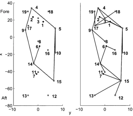
Fig. 2-1 depicts the relationships between each subject of this thesis. Conic opti-mization is the unifying tool, and is used to optimize transmission planning, recon-figuration, and ultimately approximate a new kind of multicommodity flow network
Figure 2-1: Relationships between chapters
cut.
An additional complication enters through integer variables. At present, linear and quadratic programming are the only mathematical programming frameworks with robust and efficient mixed-integer counterparts; however, as will be seen in this thesis, many mathematical descriptions of power systems are well approximated second-order cone and sernidefinite expressions, yet contain large numbers of discrete variables. Mixed-integer second-order cone programming is an active area of research for which there is the expectation of eventually achieving the sophistication of the linear analogue [46,120], and it is similarly within reason to expect subsequent devel-opment in the semidefinite case. In our discussions, we present mixed-integer linear and quadratic formulations as practical options, but also introduce mixed-integer second-order cone and semidefinite models in anticipation of future capabilities.
Chapter 3
Spectral graph theory and
multicommodity flow networks
3.1
Introduction
Spectral graph theory
[33]
offers powerful tools for analysis and design of systems which are well modeled by graphs. However, many systems have important features not captured by purely graphical descriptions. Flow networks [4,76] describe a wide variety of such systems, for example electric power grids and communication networks, yet have a minimal level detail additional to the underlying graph. In this work, we ap-ply spectral graph theory to flow networks. We formulate a class of Laplacian matrix pencils for undirected, multicommodity flow networks and a Cheeger-like parameter which generalizes the sparsest cut [90,114,119], and relate them with bounds similar to the Cheeger inequality [28,33, 42, 53]. When there are many commodities, finding the correct eigenvalue entails solving a combinatorial optimization problem, for which we formulate a semidefinite relaxation using the methodologies of [111] and [85]. In addition to flow networks, the multicommodity case may have application to many computer science problems modeled by cuts generalized by our development, such as graph partitioning [90], divide- and-conquer algorithms [114], and VLSI layout [84].3.2
Background
3.2.1
The Laplacian of a graph and the Cheeger constant
We are given an undirected, connected graph G with vertices V(G), edges E(G), and corresponding adjacency matrix A. The Laplacian of G is defined as L = D - A where D is a diagonal matrix with D,, = d, = E A,,. The normalized Laplacian is L =
D 1/2LD- 1/2, and its eigenvalues can be written 0 = A <A, < - An-1 < 2. The eigenvalues of L are equivalent to those of the generalized eigensystem Lx - ADx = 0,
which is referred to as the pencil (L, D); for convenience we use this notation [61].
A fundamental construct from which many eigenvalue results originate is known as the Rayleigh quotient [71], which we now examine. Suppose J and K are symmetric matrices, let y be a vector, and consider the equation Jy - Ky = 0. Multiplying
by yT, we have y TjY - 6yTKy = 0, and hence 6 = 2__; this ratio is known as the
Rayleigh quotient. To facilitate intuition about the mechanics employed later, we now give a basic theorem about the Rayleigh quotient:
Theorem 1 (Rayleigh-Ritz). Let 6
min be the minimum eigenvalue of the pencil (J, K),
where J and K are positive semidefinite. Then
6min = mm Y .
y y TKy
Proof. Let ... , 6,
o,
and y1, ..., y,, be the ascending-ordered eigenvalues and corre-sponding eigenvectors of (J, K). We first observe that we can equivalently minimize over vectors y for which yTKy = 1, since clearly no vector of zero length aboutK will be a minimizer if J and K are positive semidefinite. Since J and K are
y = (IYI + - - - +
(n
for some with (|| = 1. We can then writemm = min y Tjy
Y y'I'Ky y:yTKj=1
= min (61Y1 + -+ (snn)T j ( 1y1 + -+ (nyn)
O:Ilt=1
= min (61y1 + + (ny.)T K (161y1 + + (nonIYr) :I0il=1
= min (06i + - -+ 2 6ln)
001l=1In
The minimum is clearly attained for i 1 and (2 0, which completes
the proof. One can use a nearly identical argument to show that yT Jy
6max = max , . Y y2 Ky
In Section 3.4.1, we will need to take special care when the second matrix in the pencil is indefinite. The Courant-Fischer theorem [71] is a generalization of the Rayleigh-Ritz theorem, which characterizes all of the eigenvalues in the spectrum in terms of subspaces spanned by the eigenvectors. We will make immediate use of the following characterization of the second smallest eigenvalue:
62 = min j .
yY1 yTKy
We now return to the pencil (L, D). Let
f
be a function assigning a complex valuef
(v) to each vertex v, where the notationf
denotes the vector of these values. The Rayleigh quotient of (L, D) isE,-" (f(U) - f(v)) E
f
(v)2dvwhere the sum subscript u - v denotes summation over all pairs of vertices connected
satisfies
.n, Zu(f(u) - (V))2
f_LD1 f(v) 2de
The Cheeger constant [28, 33,42, 53], sometimes referred to as the conductance, is a measure of the level of bottlenecking in a graph, as illustrated in the left plot of
Fig. 3-1. It is defined
x min(vol(X), vol
(X))'
where C(X,
X)
is the set of edges with only one vertex in X, IC(X,X)
uxv, A,and vol(X) = d,. h is related to the algebraic connectivity by what is known
as the Cheeger inequality:
2h
> A
x>h
2
3.2.2
Flow networks
A flow network is a weighted graph on which flows travel between vertices by way of the edges [4, 76]. In this work we only consider undirected flow networks. Suppose further that we have a multicommodity flow network with m different types of flows or commodities [72], and that we are given a supply and demand vector for each commodity i, p , which satisfies
E
p= 0.We denote the flow of commodity i from u to v by gi(u, v), and the weight of the edge between u and v by c(u, v), which we refer to as a capacity. In this work, we equate capacities with edge weights such that the capacity of an edge, c(u, v), is identical to its weight in the graph adjacency matrix, A. We say that a flow network is feasible if there exists a flow gi : V(G) x V(G) -+ R+ satisfying E> 1 gi(u, v) <
c(u, v), and E gi(u, v) - gi(v, a) = p'.
Network flow straightforwardly model a large number of real systems, and quan-tities p' and c(u, v) deserve some concrete interpretation; as the remainder of this thesis is specific to electric power systems, which are crudely approximated by single-commodity flow networks, they are an appropriate context. The vector of supply and demand p is analogous to a vector of bus load (demand) and generation (supply). The capacity of an edge c(u, v) in this case represents a transmission line thermal
limit, restricting the flow of real or apparent power. The structure of the Laplacian matrix of capacities, L, however, has identical structure to the standard bus admit-tance matrix
[124];
here it is essentially the same matrix, but with capacities rather than admittances.For many purposes, a network with multiple sources and sinks can be reduced to one with a single source and sink by introducing a super-source and super-sink [76], for example maximizing the flow through a network. As will be seen in the next section, this simplification is not compatible with our development, and so we allow as many vertices as are in the network to be sources or sinks provided that the total flow is conserved.
3.3
A flow-based Cheeger constant
We identify a quantity which measures bottlenecking of flows rather than graphical structure, a shown in the right plot of Fig. 3-1, and is in fact a generalization of the sparsest cut [90]. We begin with the single commodity version. Define
q = min .X)I
X
vE6x PvThe denominator is the flow that would be sent from X to X in the absence of edge capacities. By the max-flow min-cut theorem, the actual flow from X to X can be no greater than
|C
(X, X) [50,75]. In fact, it is well known that q > 1 is also a sufficient condition for the existence of a feasible flow [56,70]; an implication is that q is not NP-hard when there is only one commodity.Before discussing the multicommodity case, we give a brief example for which the introduction of a super-source changes the value of q. Consider a three vertex line graph with p = [1, -2, 1]T and c(1, 2) = 3 and c(2, 3) = 2. Simple calculation gives
q = 2 and C(X,
X)
= c(2, 3) for this network. Now append a super-source with Ps 2, connected to vertices one and three by edges of unit capacity, and set pi and p3 to zero. The optimal q for the modified network is q = 1, and furthermore theC(X)
C(X.
X)
*
Sources
*
Sinks
Figure 3-1: Graph bottlenecking as measured by
h
(left) versus flow bottlenecking as measured by q (right)optimal cut has changed so that vertices one and three are now on the same side. Hence the usual simplification of multi-source, multi-sink problems to single-source, single-sink problems is not applicable here.
We now generalize q to multicommodity flow networks. Let r E {-,1}m and
p
E
p', where Wi is element i of r,, and defineS(X) = max 1 pv.
vEX
Because the objective is linear in n, it is equivalent to the continuous linear opti-mization problem in which r, E [-1, 1]". The purpose of the maximization is merely to ensure that the net-demand which would leave set X of each commodity has the same sign. We then define the multicommodity version to be
q = min (X) (
which in matrix form is given by
xT Lx
q = min L , (3.2)
reGO,1}Th,, zT
Pax|'(32where P, is a matrix with pr on the main diagonal and zeros elsewhere. q also has the minimax network flow formulation
q = minmax
r
S
77 - -7 =AK
Vv
(3.3)
0 < gO71 < AV VU -v -1 < t" < 1 Vi
Intuitively, we are optimally consolidating the supplies and demands into a single commodity, the maximum flow of which is equal to the minimum cut by the max-flow min-cut theorem and the result of
[56,70].
3.4
Laplacians for flow networks
We now derive Cheeger-like inequalities for eigenvalues of flow normalized Laplacians. Note that we have not assumed feasibility, rather only that E, p = 0 for each commodity i. The pencil (L, PK) is a natural starting point because its smallest
magnitude eigenvalue is a continuous relaxation of q. However, it is defective, which is to say that an eigenfunction is missing. It has two zero eigenvalues corresponding to the constant eigenfunction; in the simplest case of a two vertex network, the eigenvalues provide no meaningful information.
3.4.1
Variational formulation
We can see why (L, P) is defective by considering the quotient
fTPKf fTLf
It is undefined at
f
= 1, but approaches infinity asf
approaches 1 from any direction. Now consider the perturbed pencil(P,
L + al1T) for a > 0, the eigenvalues of whichare one over those of (L + aliT, P'): it is similar to vL + a11TP L + ali1, which can be real symmetric because L + al1T is positive definite. By the Rayleigh-Ritz theorem [71], the largest positive and negative eigenvalues satisfy
fTpf f Tpf
sup and inf .
f fTU(L+ a1lT)f f fT(L+ a11T)f
As a approaches zero, the two eigenvalues will approach positive and negative infinity. This is distinctly a consequence of 1 being in the null space of L and the fact that 1"P,1 = 0; were the latter not true, only one of the eigenvectors could converge to 1 and not cause the quotient to switch signs.
The zero eigenvalue of (L, P) does have a generalized eigenfunction, as guaranteed
by the Jordan canonical form theorem [71]. Solving the equation (L - OP.) x = P1 yields x = Ltp", where Lt is the Moore-Penrose pseudo-inverse of L.
We rectify (L, P,) by adding an infinite rank-one perturbation. Consider either
of the pencils limboc (L + brr', P,) and limbo (L, P, + brrT), where r E R" is not orthogonal to 1. They will respectively have an infinite and a zero eigenvalue, both corresponding to the eigenfunction r, and will share the remaining eigenvalues and eigenfunctions.
Because both matrices of the pencil are real symmetric and the left matrix is positive definite, the eigenvalues and eigenfunctions are real and admit a variational characterization. The magnitude of the smallest, which we denote p, has the
varia-tional characterization pr =Jiminf fT (L + brrT) f b-+c~o f [Tp 1 fILf (4) = inf . (3.4) f1r fTPJ Define
= min
/.
(3.5)Even for the simple case in which r is not a function of r,, a continuous relaxation of (3.5) is not guaranteed to have a unique global minimum. This is evident from the reciprocal
(p) =1 max sup f
T ,~f
fir fTLf
which is the maximum of the pointwise supremum of a family of linear functions of
K, and hence a convex maximization problem [25]. A consequence is that there is
no easy way of computing pf when there are many commodities; however, when the number of commodities is small, it may be straightforward to guess the optimal K, or simply try all of the likely ones. Furthermore, convexity does guarantee that the optimal K is at a corner, and thus the continuous relaxation is equivalent to the binary formulation.
3.4.2
Bounds on p'
We have the following Cheeger-like inequality:
Theorem 2.
q | rv| >r> qh JE re|
vEX rv - vG r| 2 ( dv v |r |/dv'
where X is the vertex set associated with q and r E R".
Proof. The structure of our proof for the most part follows that of the Cheeger
extends to networks with non-negative capacities by generalizing the definition of the Laplacian to allow for weighted graphs.
We begin with the upper bound. Define the function
f(v) =
ZEX,r
1if vEX
-
Eg
raif ) (E X-
ZUEXTrU i*~where X is the optimal vertex set associated with q. Let ri and r12 be optimal for (3.1) and (3.5), respectively. Substituting
f into (3.4) gives
r
- C
(X)
(ZICX rV + Evcg r )2q
E, r,)I
EE u- ZEqk& rV
We now prove the lower bound. Let
f
be the eigenfunction of limbo(L +brrT, P) associated with p . Order the vertices in V(G) so that
If(vi) I
If(vi+1)|for i = 1, ... ,I n-1. For each i define the cut Di {{j,k}
E E(G)
I
1 <j i < k < n},and set
a = minD
Isi<n 2
By definition, ac
>
q regardless of whether or not i, = 2. We haver
E
~, (f(v) - f (U))2 E (f(v) + f(U))2P:f (v)
2p? E_,
(f (u)
+ f (V))2
(E
If(u)
2 -f (V)212
2E f (V)2pr? E" f (V)2dv __(ZI
f(v) 2 - f(v+1)2| D 1) 2 2 f(v) 2 p'2E"
f(v) 2dv by Cauchy-Schwartz by counting - (EVEg rV S(X) (Y:EX 7-r )2f(v,)
2f
(vi+1)2)
aL
p
)2 2E,f
(v)2p'2LV
f
(v)2d 2(i(f (V,)
2 -f (V,+1)
2)
z
3
12)2
L,
f(v)
2pg2 J, f(v) 2dvq
2(zi
f(v )
2(Li
pK2
-2> fv)
2p!2LV
f(v)2dvq
2(L f (7v,2 2EL
f
v
)2p 2L
q2 f (V) 2 p 22
Lv
f (v)2dv by the definition of aby the triangle inequality
V-2
)
)
2f(v)
2dvSwitching to matrix notation and noting that P'ffTP 2f - -f
TLf, we simplify further so that
q2fTLf
2prfT Df
Multiplying through by pIr and taking the positive square root, we have that
r > q
fTLf2fTDf > q
where Ar is the smallest eigenvalue of the pencil limbso(L + brrT, D).
A, may not be an intuitive quantity in some cases, so we also derive a slightly looser but more revealing lower bound, which is a function of A, and thus h, by the Cheeger inequality. Using similarity and the substitution I = Di1/2f, we have
y q 2l l ^
Because D1
projection onto the orthogonal complement of D1121, which we denote projD1/21 1)
The minimum possible ratio of their lengths is given by
m
m I
|projD1/21
1L)(C) 1m
i
- projDl/21(C)I(36)
cLD -1/2r 11C11 cLD -1/2r IlCil
The minimizing c is
-=
projD-1/2r1(D
1/21) = Di/21 - projD-1/2r(D
1/21)Substituting , into (3.6), after some algebra, yields
|1TTri
I,r,|
IDi/21||||JD-1/2r|| g/E
d-
*,r2d
Let k be a vector the same length as I and parallel to projD1/21 1 (1). We then have
,tr > q03 kTEk
V
21TJ 2 q 21111 12 q0 qhp 23.4.3
Orthogonality constraints
It is important that the upper bound stays finite for all networks of interest; for some
r, there are certain networks which will cause the denominator to be zero, constituting
an effective blindspot in ptr. For analysis of a single network, one might heuristically construct an r for which it is clear that this can not happen. Design and optimization however require that the upper bound remains finite for all possible networks, or else
We now examine several choices of r.
1. The maximum possible lower bound is qh/2, which is attained by r = D1. Unfortunately, the upper bound then becomes
itD1 qvol (V(G))
v-
Vol(X) - vol
(X)I'
which is infinite if the sums of the degrees on either side of C (X,
X)
are equal. This is reflected in p D1 as well: consider a symmetric 'dumbbell' network inwhich two identical halves are connected by a single edge, and assume that all vertices in one half are unit sources and in the other half unit sinks of a single commodity. As the size of the halves is increased, it can be observed that 1 D1 grows despite qi decreasing as one over the number of vertices.
2. q has a number of interpretations in which being larger is better, so we are interested in choices for which it is the only non-constant factor in the upper bound. Let Y C X or Y C X. If we choose r to be
if V Y (3.7)
0 if v G Y
the bound becomes
q y qh vol(Y) 2 vol(V(G))
This may somewhat impractical for most choices of Y, particularly in contexts
in which the edges and hence X can change. However, if Y is the singleton z, X need not be known, and vol(Y) is simply replaced by d2. The formulation is
simple in this case, but the dependence on the vertex z and the potential 1/fn factor in the lower bound may be undesirable.
3. Rather than using a single orthogonality constraint, taking the minimum of two eigenvalues can result in an upper bound which is always finite. For a vertex set N, let N+ (N-) denote the subset for which p"' > 0 (pgi < 0), 7) e N, where
Ki is optimal for (3.1). Consider
{
p
v E V(G)+
_
pK
s 0 and s 0
0 v E V(G)~ 0
and set W = min {p*, p" }. The upper bound of the minimum of the two resulting eigenvalues is P18 < min q ZvEV(G)+ PVK;i ZVEX+ Pr7) -
ZIIE)+
Pr1 EXEV(G)-
PvJ
Observe that 2S(X) vEX >§ K1 VEX+Because the numerators are equal, we have
13 q Ev |pglI| p <
-- 2S(X)
which is finite because S(X) is always greater than zero. Under certain con-ditions, p" is bounded above by q, as shown in the computational example in Section 3.7.1 and by the following lemma.
Lemma 1. Suppose V(G)+
C
X or V(G) C X. Then I < q.Proof. Let P+
(P-)
be a matrix with s+ (s-) on the main diagonal and zeros elsewhere, and let x be the minimizer of (3.2). We haveSxT Lx q =


![Figure 4-1: 46-bus Brazilian system (from [68]). Dashed lines represent candidate ad- ad-ditions without existing lines, and solid lines existing lines (which are also candidates for additions).](https://thumb-eu.123doks.com/thumbv2/123doknet/14454608.519377/75.918.247.693.208.806/figure-brazilian-represent-candidate-existing-existing-candidates-additions.webp)
![Figure 4-2: 24-bus IEEE reliability test system (from [96])](https://thumb-eu.123doks.com/thumbv2/123doknet/14454608.519377/76.918.252.736.152.856/figure-bus-ieee-reliability-test-system-from.webp)
![Table 4.2: Garver's six bus system Model NL [106] LAC, T 2 = 1 LAC, 'r 2 = 0](https://thumb-eu.123doks.com/thumbv2/123doknet/14454608.519377/77.918.283.634.324.544/table-garver-six-bus-system-model-lac-lac.webp)
![Figure 4-3: Candidate with existing networks (solid) and candidate without existing networks (dashed) in Garver's six bus system (from [107])](https://thumb-eu.123doks.com/thumbv2/123doknet/14454608.519377/78.918.249.720.210.801/figure-candidate-existing-networks-candidate-existing-networks-garver.webp)