On the computation of viscous terms for incompressible two-phase flows with Level Set/Ghost Fluid Method

HAL Id: hal-01308135

https://hal.archives-ouvertes.fr/hal-01308135

Submitted on 27 Apr 2016

HAL is a multi-disciplinary open access

archive for the deposit and dissemination of

sci-entific research documents, whether they are

pub-lished or not. The documents may come from

teaching and research institutions in France or

abroad, or from public or private research centers.

L’archive ouverte pluridisciplinaire HAL, est

destinée au dépôt et à la diffusion de documents

scientifiques de niveau recherche, publiés ou non,

émanant des établissements d’enseignement et de

recherche français ou étrangers, des laboratoires

publics ou privés.

On the computation of viscous terms for incompressible

two-phase flows with Level Set/Ghost Fluid Method

Benjamin Lalanne, Lucia Rueda Villegas, Sébastien Tanguy, Frédéric Risso

To cite this version:

Benjamin Lalanne, Lucia Rueda Villegas, Sébastien Tanguy, Frédéric Risso. On the computation

of viscous terms for incompressible two-phase flows with Level Set/Ghost Fluid Method. Journal

of Computational Physics, Elsevier, 2015, vol. 301, pp.289-307. �10.1016/j.jcp.2015.08.036�.

�hal-01308135�

O

pen

A

rchive

T

OULOUSE

A

rchive

O

uverte (

OATAO

)

OATAO is an open access repository that collects the work of Toulouse researchers and

makes it freely available over the web where possible.

This is an author-deposited version published in :

http://oatao.univ-toulouse.fr/

Eprints ID : 14504

To link to this article : DOI :

10.1016/j.jcp.2015.08.036

URL :

http://dx.doi.org/10.1016/j.jcp.2015.08.036

To cite this version : Lalanne, Benjamin and Rueda Villegas, Lucia

and Tanguy, Sébastien and Risso, Frédéric On the computation of

viscous terms for incompressible two-phase flows with Level Set/Ghost

Fluid Method. (2015) Journal of Computational Physics, vol. 301.

pp.289-307. ISSN 0021-9991

Any correspondance concerning this service should be sent to the repository

administrator:

staff-oatao@listes-diff.inp-toulouse.fr

On

the

computation

of

viscous

terms

for

incompressible

two-phase

flows

with

Level

Set/Ghost

Fluid

Method

Benjamin Lalanne,

Lucia Rueda Villegas,

Sébastien Tanguy

∗

,

Frédéric Risso

InstitutdeMécaniquedesFluidesdeToulouse,UniversitédeToulouseandCNRS,AlléeCamilleSoula,31400Toulouse,France

a

b

s

t

r

a

c

t

Keywords:

LevelSet GhostFluidMethod Two-phaseflows Viscosityjumpcondition

Inthispaper,wepresentadetailedanalysisofthecomputationoftheviscoustermsforthe

simulation ofincompressible two-phaseflows intheframework ofLevelSet/GhostFluid

Method whenviscosity isdiscontinuousacrossthe interface. Twopioneering paperson

thetopic,Kangetal.[10]and Sussmanetal.[26],proposedtwodifferentapproachesto

deal with viscous terms. However, adefinitive assessmentof theirrespective efficiency

iscurrently notavailable. Inthispaper,wedemonstratefromtheoreticalargumentsand

confirm from numerical simulations that these two approaches are equivalent from a

continuous point of view and we compare their accuracies in relevant test-cases. We

alsoproposeanew intermediatemethodwhichusesthepropertiesofthetwoprevious

methods. Thisnew method enables asimple implementation for an implicit temporal

discretizationoftheviscousterms.Inaddition,theefficiencyoftheDeltaFunctionmethod

[24]isalsoassessedandcomparedtothethreepreviousones,whichallowustopropose

ageneraloverviewoftheaccuracyofallavailablemethods.Theselectedtest-casesinvolve

configurationswhereinviscosityplaysamajorroleandforwhicheithertheoreticalresults

orexperimental dataare availableasreference solutions:simulations ofsphericalrising

bubbles,shape-oscillatingbubblesanddeformedrisingbubblesatlowReynoldsnumbers.

1. Introduction

In pioneering works on simulation of incompressible two-phase flows with interface tracking or interface capturing algo-rithms,discontinuitiesofpressurefield,densityfieldorviscosityfieldweretackledbysmoothingthesingulartermsacross theinterfaceonafinitelayerofabout2or3gridcellsthick.Thiskindofapproacheshasbeenproposedintheframework of Front-Tracking algorithms[1,30], for Volume-of-Fluid methods[6,12], and for Level-Set methods[24]. In the literature, they

arereferred toasContinuumSurfaceForcemethods orDeltaFunctionmethods.Such methodsstillprovidesatisfactoryresults inmanysituations.Nevertheless,theysufferfromsomedrawbackssuchasthepresenceofintensespuriouscurrentsathigh capillary-numbers, which can induce strong numerical instabilities. Also, they have to face the tricky problem of describing a surface as a volume of small thickness. A few years ago, a new class of method appeared in the literature, where singular terms across an interface are treatedasjumpconditions, whichprevents frominterface thickening aswell asit reduces spurious currents. Significant contributions to thisnewapproach, well known asSharpInterfacemethod, can be found in

[21] for Front-Tracking methods,in [10,15,26]for Level-Set methods,and [5] Volume-of-Fluid methods.In [26], a Level-Set

method was coupled witha Volume-of-Fluid method,butthe way to impose thejump conditions dependedonly onthe

*

Correspondingauthor.Tel.:+33534322808;fax:+33534322899.

E-mailaddress:tanguy@imft.fr(S. Tanguy).

Level-Setfunction–thevolumefractionbeingjustusedtoimproveinterfaceadvectionandtocomputeinterfacecurvature. Most of these papers emphasize on improvements resulting from a sharp description of the surface tension, but they are not conclusive about the effectivenessofSharp Interfacemethods forthe discretizationof viscous terms.However, Kang etal.[10] proposed a newdiscretization oftheviscous terms basedon thegeneral principleof theGhost FluidMethod

[4,15]. The main feature of this new approach consists in computing the contraction of the divergence of the viscous stress

tensorina Laplacianoperatorofthe velocitycomponents

µ

1 E

V ratherthan itsfull expression (with

µ

thedynamic vis-cosity and _{V the}

E

_{velocity field). This contraction is only possible for incompressible flow when viscosity is uniform; it is}

henceapparentlynotsuitedtocompute theviscoustermsongridcellsthat arecrossedby aninterfacebetweentwo dif-ferentfluids. Tosolvethisissuefortwo-phaseflows,once

µ

1 E

V hasbeencomputed,theauthorsproposetoaddexplicitly the jump of the normal viscous stresses at the interface, resulting from the jump of viscosity, to the pressure jump while solvingthePoissonequation forthepressure.Anotherapproach tocomputethe viscoustermsintheframework ofSharp Interface methods, inspired of a previous work [15], was proposed by Sussman et al. [26]. In a similar way of what it is

usuallydoneinContinuumSurfaceForce methods,thefullexpressionofthedivergenceoftheviscousstresstensor

∇.(

2µD

)

isdiscretized,theviscousstresstensorbeingdefinedby2µD foraNewtonianfluid,withD therate-of-deformationtensor. In this approach, contrary to previous work [10], it seems that the contribution of the normal viscous stresses has not to be

addedexplicitlytothepressurejumpconditionattheinterface.Valuablenumericalvalidationsofthismethodareproposed in [26]. However, whether these two approaches are formally equivalent or not remained an open question. In particular,

thefactthat jumpofthenormalviscous stresseshastobeexplicitlyaddedto thepressurejumpin[10] andnot in[26]

still required to be justified.

In this paper, we focus on the computation of viscous terms for incompressible two-phase flows using Level-Set methods.

IntheframeworkofSharp-Interface methods,weshalldemonstratethatthetwoapproachesintroducedin[10] and[26]

are equivalent from a theoretical point of view, even if their numerical implementation is quite different.

Fromthisoriginaldemonstration,anewintermediatemethodisproposed,whichallowstomakemoreeasilytheimplicit temporal discretization of the viscous terms as the two methods proposed in [10]and [26].

To complete this survey of numerical methods, we also discuss the consistency of these three Sharp-Interface methods

withtheDelta-Function methodthatisbasedonaContinuumSurfaceForce approach.

Section 2describes the formalism of this set of four methods and proves their equivalence. Then, Section 3 proposes

three numerical benchmarks that are particularly relevant to assess the reliability of these methods and compare their accuracy: spherical rising bubbles, damped shape oscillations of a bubble, and deformed rising bubbles at low Reynolds number.

2. Equations&numericalmethods

2.1. Equationofmotionfortwo-phaseflows,jumpconditionandsingularsourceterm

Let us consider the Navier–Stokes equations for a single-phase incompressible flow; the following two equations express respectivelymomentumandmassconservation:

ρ

DV

E

Dt

= −∇

p

+ ∇ · (

2

µ

D

) +

ρ

E

g

,

(1)

∇ · E

V

=

0

,

(2)

whereV is

E

thevelocityfield, _DtD istheLagrangianderivative,

ρ

isthefluiddensity,

µ

isthefluidviscosity,p isthepressure field,

E

g is

the gravity acceleration, and

D is

the rate-of-deformation tensor defined as:

D

=

∇ E

V

+ ∇ E

V

T

2

.

(3)

For incompressible flows with constant viscosity, it can be easily shown that:

∇ · (

2

µ

D

) =

µ

1 E

V

,

(4)

which leads to the following simplified expression for Navier–Stokes equation:

ρ

DV

E

Dt

= −∇

p

+

µ

1 E

V

+

ρ

E

g

.

(5)

Letusnowconsideranincompressibletwo-phaseflow,thewhole-domain-formulation[1,23]leadstothefollowing expres-sion that includes the capillary forces:

ρ

DV

E

Dt

= −∇

p

+ ∇ · (

2

µ

D

) +

σ κ

n

E

δ

Γ

+

ρ

E

g

,

(6)

where

σ

isthesurfacetension,

κ

istheinterfacecurvature,n is

E

thenormalvectorattheinterfaceand

δΓ

isa multidimen-sionalDiracdistributionlocalized attheinterface. Ifnophase changeoccurs, eq.(2)stays valid. Asdensityandviscosity can vary the across interface, they can be defined as:

ρ

=

ρ

gas

+ (

ρ

liq

−

ρ

gas

)

HΓ

=

ρ

gas

+ [

ρ

]

ΓHΓ

,

(7)

µ

=

µ

gas

+ (

µ

liq

−

µ

gas

)

HΓ

=

µ

gas

+ [

µ

]

ΓHΓ

,

(8)

where HΓ is aHeaviside distribution,equalto 1intheliquidphase andequalto0 inthegasphase, withthe following

definitions for density and viscosity jump conditions:

[

ρ

]

Γ

=

ρ

liq

−

ρ

gas

,

(9)

[

µ

]

Γ

=

µ

liq

−

µ

gas

.

(10)

Moreover, considering a divergence-free condition on the velocity field, the following unsteady advection equation for the densityfieldisobtainedfrommassconservation:

D

ρ

Dt

=

0

.

(11)

From that equation, we candeducethe usual propagationequation forinterface motionthat canbe used withLevel Set methods:

D

φ

Dt

=

0

,

(12)

where

φ

isasigneddistancefunctionfromtheinterface.NotethatanothersimilarequationcanbederivedforVolumeOf Fluidmethods:

DF

Dt

=

0

,

(13)

where F is

the local volume fraction of the considered phase in a computational cell.

Thebalanceofnormalstressesattheinterfaceinvolvesajumpofpressureandajumpofnormalviscousstresses:

[

p

]

Γ

=

σ κ

+

2

[

µ

]

Γ

∂

Vn

∂

n

.

(14)

Letusremarknowthattheviscous-stresstensorcanbesplitintotwoparts:

∇ · (

2

µ

D

) =

µ

∇ · (

2D

) +

2D

· ∇

µ

.

(15)

Ifviscosityisapiecewiseconstant,byusingthedefinitionoftheHeavisidederivative,itcanbeshownthat:

∇

µ

= [

µ

]

Γ

E

n

δ

Γ

.

(16)

Finally,weobservethattheprevioussplitting(15)isadecompositionoftheglobalviscousterminacontinuouspartanda singularpart(zeroeverywhereexceptattheinterface):

∇ · (

2

µ

D

) =

µ

1 E

V

+

2

[

µ

]

ΓD

· E

n

δ

Γ (17)

This highlights that the contribution of the viscous terms on the pressure jump is already included in the left-hand side ofeq. (17).Thus, wecan supposethat computingthedivergenceoftheoverallviscous stress tensorallowsincludingthe contributionofviscous effectsinthepressurejump.Amore rigorousproof ofthatassertion isprovidedinSection 2.4of this paper.

Tosummarize,themomentumequationcan bedefinedinawhole-domainformulation leadingtoeq.(6)withadensity and a viscosity field defined respectively by eqs. (7) and(8), or in a jump-conditionformulation leading to eq. (5) with additional jump conditions(9), (10), (14).

2.2. Aboutthelinkbetweenjumpconditionsandsingularsourceterms

Letusconsideravolume

Ω

,boundedbyasurface

Σ

,anddefinedas

Ω

1U

Ω

2,wherethetwosubdomains

Ω

1 and

Ω

2

areseparatedbyaclosedsurface

Γ

with

Γ ∩ Σ = ∅

,asillustratedinFig. 1.Wedefinen

E

1 andn

E

2 asthenormalvectorsat

the surface

Γ

pointing respectively towards

Ω

1and

Ω

2.

Let us now consider a piecewise continuous function

ψ

which respects the Poisson equation,

1ψ =

0 (18)

inside both subdomains

Ω

1 and

Ω

2, with the following jump condition at the interface:

[ψ]

Γ

=

a

(E

xΓ

),

(19)

where a

(E

xΓ

)

is a function of the interface coordinate

E

xΓ. The jump condition(19)involves that the following surface integral

Fig. 1.Sketch of a two-phase flow domainΩ1UΩ2with an immersed interfaceΓ.

¨

Γ

¡[ψ]

Γ

−

a

(E

xΓ

)¢E

n2dS

= E

0 (20)

Considering a homogeneous Dirichlet boundary condition on the external boundary

Σ

of the computational field, it can be

easilydemonstratedthat

¨

Σ

ψ E

nΣdS

=

0

,

(21)

wheren

E

Σ isthenormalvectorpointingoutwardstheexternalboundary

Σ

.Thus

¨

Σ

ψ E

nΣdS

+

¨

Γ

¡[ψ]

Γ

−

a

(E

xΓ

)¢E

n2dS

=

0

.

(22)

Moreover,byremarkingthat

¨

Γ

¡[ψ]

Γ

−

a

(E

xΓ

)¢E

n2dS

=

¨

Γ

ψ E

n2dS

+

¨

Γ

ψ E

n1dS

−

¨

Γ a

(E

xΓ

)E

n2dS (23)

we obtain the following equality:

¨

Σ

ψ E

nΣdS

+

¨

Γ

ψ E

n2dS

+

¨

Γ

ψ E

n1dS

=

¨

Γ a

(E

xΓ

)E

n2dS

.

(24)

Eq.(24)can also be written as

˚

Ω1

∇ψ

d

Ω +

˚

Ω2

∇ψ

d

Ω =

˚

Ω

∇ψ

d

Ω =

˚

Ω a

(E

xΓ

)E

n2

δ

Γd

Ω,

(25)

which leads to the following local formulation:

∇ψ =

a

(E

xΓ

)E

n2

δ

Γ

.

(26)

Finally,afterdifferentiation,weobtain:

1ψ = ∇ ·

¡

a

(E

xΓ

)E

n2

δ

Γ

¢.

(27)

Wehavethereforeshownthataddingthefollowingsourceterm

∇ · (

a

(E

xΓ

)E

n2

δΓ

)

totheright-handsideofaPoissonequation

imposes a jump condition

[ψ]

Γ

=

a

(E

xΓ

)

on its solution

ψ

. This is also valid for a Poisson equation like eq. (18) with a

right-hand side different from zero.

Moreover,followingasimilarapproach,itcanalsobedemonstratedthat ascalarfieldthatissolutionofthefollowing equation

1ψ =

b

(E

xΓ

)δ

Γ

,

(28)

withb

(E

xΓ

)

anotherfunctiondependingoninterfacecoordinate,willalsofulfillsthefollowingjumpcondition:

[E

n2

· ∇ψ] =

b

(E

xΓ

).

(29)

2.3. Projectionmethodfor whole-domainformulationand jump-conditionformulation

Let us consider now a first-order explicit projection method for the single-phase incompressible Navier–Stokes equation. Itconsistsinprescribingafirstintermediate velocityfieldwhichdoesnotrespectthedivergence-freecondition(predictor step):

E

V₁∗

= E

Vn

− 1

t

¡¡

_E

Vn

· ∇

¢

_E

Vn

−

υ

1 E

Vn

− E

g

¢,

(30)

with

υ

thekinematicviscosity.

Next,aPoissonequationmustbesolvedtodeterminethepressurefield:

1

pn+1

=

ρ

n+1

∇ · E

V

∗

1

t

.

(31)

Then, in a last step, the final divergence-free velocity field can be computed using the pressure field determined at the previous step:

E

Vn+1

= E

V∗

− 1

t

∇

p

n+1

ρ

n+1

.

(32)

Applying the projection method toan incompressible two-phase flow isless straightforward. Dependingon whether the

whole-domainformulation orthejump-conditionformulation isused,theintermediatevelocityinthefirststepofthe projec-tion method has to be different.

Let us first consider a whole-domainformulation. An explicit temporal discretization of the capillary and viscous terms

leadsquitenaturallytothefollowingpredictorstep

E

V₂∗

= E

Vn

− 1

t

µ

¡

_E

Vn

· ∇

¢

_E

Vn

−

∇ · (

2

µ

D n

₎

ρ

n+1

−

σ κ

n

E

δ

Γ

ρ

n+1

− E

g

¶

,

(33)

withthecorrespondingPoissonequation

∇ ·

µ

∇

pn+1

ρ

n+1

¶

=

∇ · E

V ∗ 2

1

t

= ∇ ·

µ

E

Vn

− 1

t

µ

¡

_E

Vn

· ∇

¢

_E

Vn

−

∇ · (

2

µ

D n

₎

ρ

n+1

−

σ κ

E

n

δ

Γ

ρ

n+1

− E

g

¶¶

.

(34)

Next,thecorrectionstepgives:

E

Vn+1

= E

V₂∗

− 1

t

∇

p

n+1

ρ

n+1

.

(35)

Letusnowconsidertheapplicationoftheprojectionmethodtoajump-condition formulation oftheNavier–Stokesequation. We have to solve eq.(5), so the first step of the projection method is similar to eq.(30)for a single-phase flow. As we want

toimpose theappropriatejumpconditionattheinterfaceonthepressurefield (eq.(14)),we canshow,usingtheresults presentedinSection2.2,thatitcanbedone bysolvingthefollowingPoissonequation forthepressurewitharight-hand side split into a continuous part and a singular part:

∇ ·

µ

∇

pn+1

ρ

n+1

¶

=

∇ · E

V ∗ 1

1

t

+ ∇ ·

µ (

σ κ

+

2

[

µ

]

Γ∂∂Vnn

)E

n

δ

Γ

ρ

n+1

¶

.

(36)

Using the splitting of the viscous term given ineq. (17)and notingthat n

E

·

D

· E

n

=

∂Vn

∂n , we find the following relation

between _V

E

∗ 2 and V

E

1∗:

E

V₂∗

= E

V₁∗

+ 1

t

(

σ κ

+

2

[

µ

]

Γ ∂Vn ∂n

)E

n

δ

Γ

ρ

n+1

.

(37)

The use of eq.(37)allows demonstrating that eq.(34)and eq.(36)are formally identical:

∇ ·

µ

_∇

_pn+1

ρ

n+1

¶

=

∇ · E

V ∗ 2

1

t

=

∇ · E

V₁∗

1

t

+ ∇ ·

µ (

σ κ

+

2

[

µ

]

Γ∂_∂V_nn

)E

n

δ

Γ

ρ

n+1

¶

.

(38)

Then,by consideringeq.(37),we candeducethefollowingcorrectionstepforajump-conditionformulation,leading tothe same field _V

E

n+1 _{than in eq.(35):}

E

Vn+1

= E

V₁∗

−

1

t

ρ

n+1

µ

∇

pn+1

−

µ

σ κ

+

2

[

µ

]

Γ

∂

Vn

∂

n

¶

E

n

δ

Γ

¶

.

(39)

To summarize,we have shownthatboth a whole-domainformulation and a jump-conditionformulation canbe used when applying a projection method to an incompressible two-phase flow. These two methods are formally equivalent, but they

leadtoadifferentdefinitionofthepredictedvelocityfield inthefirststepoftheprojectionmethod.In[10],the interme-diate velocity field _V

E

∗

1 is used, whereas in [1,3,6,24] it is the intermediate velocity field V

E

2∗. These two methods will be

respectively named in the rest of this paper the Ghost-FluidPrimitiveviscousMethod (GFPM)

and the

Delta-FunctionMethod

(DFM).

2.4.Projectionmethodforintermediateformulations

Other definitionsofthepredictedvelocityfieldarepossible.Forexample,weproposethefollowingtwo definitions,the respective interests of which will be discussed later:

E

V₃∗

= E

Vn

− 1

t

µ

¡

_E

Vn

· ∇

¢

_E

Vn

−

∇ · (

2

µ

D n

₎

ρ

n+1

− E

g

¶

,

(40)

E

V₄∗

= E

Vn

− 1

t

µ

¡

_E

Vn

· ∇

¢

_E

Vn

−

∇ · (

µ

∇ E

V n

₎

ρ

n+1

− E

g

¶

.

(41)

In the same way as in the previous section, they lead to the definition of these two Poisson equations, formally equivalent to eq.(34)and eq.(36):

∇ ·

µ

_∇

_pn+1

ρ

n+1

¶

=

∇ · E

V ∗ 3

1

t

+ ∇ ·

µ

σ κ

n

E

δ

Γ

ρ

n+1

¶

,

(42)

∇ ·

µ

∇

pn+1

ρ

n+1

¶

=

∇ · E

V ∗ 4

1

t

+ ∇ ·

µ (

σ κ

+ [

µ

]

Γ∂_∂V_nn

)E

n

δ

Γ

ρ

n+1

¶

.

(43)

Thefollowingrelationshavebeenusedtodetermineeq.(43):

∇ · (

2

µ

D

) = ∇ ·

¡

µ

¡∇ E

V

+ ∇

T_V

_E

_{¢¢ = ∇ · (}

_µ

_{∇ E}

_V

_{) +}

_µ

_{∇ · ∇}

T_V

_E

_{+ ∇}

_µ

_{· ∇}

T_V

_E

_,

₍₄₄₎

∇ · (

2

µ

D

) = ∇ · (

µ

∇ E

V

) + [

µ

]

Γ

∇

TV

E

.E

n

δ

Γ

,

(45)

since

∇.∇

T_V

_E

₌

_{0 for an incompressible flow, and}

E

n

.∇

TV

E

.E

n

=

∂

Vn

∂

n

.

(46)

Then,thetwofinalcorrectorsteps,respectivelysuitablewitheq.(40)andeq.(41),are:

E

Vn+1

= E

V₃∗

−

1

t

ρ

n+1

¡∇

p n+1

₋

_{σ κ}

_n

_E

_δ

Γ

¢,

(47)

E

Vn+1

= E

V₄∗

−

1

t

ρ

n+1

µ

∇

pn+1

−

µ

σ κ

+ [

µ

]

Γ

∂

Vn

∂

n

¶

E

n

δ

Γ

¶

.

(48)

The intermediate velocity field V

E

₃∗ hasalready been used inRefs. [5,21,26]in the framework of SharpInterfacemethods.

In the rest of this paper, the Ghost-FluidConservativeviscousMethod (GFCM)

will

refer to the numerical method proposed

in [26]. Finally, the use of V

E

₄∗ leads to an original numerical method to deal with the viscous terms, that we name the Ghost-FluidSemi-ConservativeviscousMethod (GFSCM).

The four methods DFM, GFPM, GFCM and GFSCM described above are therefore theoretically equivalent, but they lead to different numerical approximations. The next objective of this paper is to discuss about their respective interests and numericalaccuracy.

2.5.Spatialdiscretizationofsurfacetension

When a whole-domainformulation [3,6,12,24,30] is used, the surface-tension singular term isaccounted for when V

E

₂∗

is computed. The intermediate velocity field is next differentiated to compute the right-hand side of the pressure Poisson equation.Therefore,itiswellsuitedtoasmoothdiscretizationofthesurface-tensiontermthatinvolvesafictitiousinterface thickness. Its application to a sharp-interface description would be trickier. This approach is that of the Delta-Function Method,

known as

ContinuumSurfaceForce method.

In this framework, the numerical discretization of

discontinuous terms

makesuseofthefollowingregularizedsmoothedHeavisidefunctiondefinedfromtheLevel-Setfunction

φ

:

Hε

(φ) =











0 if

φ < −

ε

1 2

¡

1

+

φ_ε

+

sin( πφ ε ) π

¢

if

|φ| ≤

ε

1 if

φ > +

ε

,

(49)

where

ε

is the fictitious interface thickness, which is equal to 2 or 3 cell sizes. The surface-tension termcan then be computed using the following approximation:

σ κ

n

E

δ

Γ

∼

=

σ κ

∇

Hε

.

(50) At the opposite, a projection method using a jump-conditionformulation with V

E

₁∗ as intermediate velocity field is well suitedforSharp-Interfacemethods.Thankstothisformulation, artificialsmoothingofinterfacesingularitiescanbe avoided, allowing a sharp-interface description. It has been used in the framework of Ghost-FluidMethod in [15], where authors

propose afirst-orderdiscretization toimposea jumpconditiontothe solutionaswellastothe normalderivativeof the solution when solving the Poisson equation

∇ · (β∇

u

) =

f

,

(51)

i.e. with the following interface jump conditions

[

u

] =

a

(E

xΓ

)

and

·

β

∂

u

∂

n

¸

=

b

(E

xΓ

).

Considering that capillary effects can be computed as a jump condition on pressure, an original Sharp-Interfacemethod for

solving the Navier–Stokesequation inthe framework ofLevel-Setmethods was introduced in[10].This methodhas been widely used to perform direct numericalsimulations oftwo-phase flows [16,26–29]. Letus now briefly summarize this approach.

Thediscretizationofa2DPoissonequationaseq.(51),whichinvolvesadiscontinuityofthesolutionandofitsnormal derivative at the interface, writes:

β

i+1/2 j

(

ui+1 j−ui j 1x

) − β

i−1/2 j

(

ui j−ui−1 j 1x

)

1

x

+

β

i j+1/2

(

ui j+1 −ui j 1y

) − β

i j−1 2

(

ui j−ui j−1 1y

)

1

y

=

fi j

+

gi j

+

hi j

,

(52)

where interpolations of the diffusion coefficient

β

on the cell borders are computed as the harmonic average of its value

β

+ intheregion wherethe LevelSet functionis positiveandits value

β

− in theregion wheretheLevel Setfunction is negative; for example, if the interface crosses a mesh segment between xi and xi+1:

β

i+1/2 j

=

β

+

β

−

β

+

θ + β

−

(

1

− θ)

,

(53) with

θ =

|φ

i+1 j

|

|φ

i+1 j

| + |φ

i j

|

.

(54)

Thesourceterms gi j andhi j intheright-handsideofeq.(52)matchwiththediscontinuitiesofu andof

β

∂_∂un;theycanbe

computed as

gi j

=

gi jR

+

gi jL

+

gi jT

+

gBi j

,

(55)

hi j

=

hi jR

+

hLi j

+

hTi j

+

hi jB

,

(56)

whereeachofthesetermsarenon-zerowhenan interfacecrossesthecorrespondinggridsegment,andsuperscripts R,L, T ,B denoterespectivelyright,left,topandbottomsides.Theirexpressionsare:

g_{i j}R

= ±

β

i+1/2 jaΓ

1

x2 g L i j

= ±

β

i−1/2 jaΓ

1

x2 g T i j

= ±

β

i j+1/2aΓ

1

y2 g B i j

= ±

β

i j+1/2 jaΓ

1

y2

,

(57) hR_{i j}

= ±

β

_i+1 2jbΓ

θ

β

±

1

x h L i j

= ∓

β

_i−1 2jbΓ

θ

β

±

1

x h T i j

= ±

β

_{i j+}1 2bΓ

θ

β

±

1

y h B i j

= ∓

β

_{i j−}1 2bΓ

θ

β

±

1

y

.

(58)

It is noteworthy that an analogy can be established by using the results demonstrated in Section 2.2and the discretization

described in thissection. Forsake ofsimplicity,let ustake a diffusioncoefficient

β

equal tounity. InSection 2.2,it has beenshownthatsolving

1

u

=

f with

[

u

] =

a

(E

xΓ

)

and

· ∂

u

∂

n

¸

=

b

(E

xΓ

)

is equivalent to solve

1

u

=

f

+ ∇.

¡

a

(E

xΓ

)E

n

δ

Γ

¢ +

b

(E

xΓ

)δ

Γ

.

Comparingthisexpressionwithdiscreteequation(52),wededucethatsourceterms gi j andhi j,thatappearinthe

frame-work of the Ghost-FluidMethod,

are respectively numerical approximations of

∇.(

a

(E

xΓ

)E

n

δΓ

)|

i j and b

(E

xΓ

)δΓ

|

i j:

∇ · (

an

E

δ)|

i j

=

gi j

+

O

(1

x

)

(59)

b

δ|

i j

=

hi j

+

O

(1

x

)

(60)

Such ananalogyestablishesthelinkbetweentheContinuumSurfaceForce approachbasedonnumericalapproximationsof

2.6.Spatialdiscretizationofviscousterms

More details are provided in this section about the spatial discretization of viscous terms for the different methods described in the previous sections. In the following, for sake of simplicity, all developments are presented in 2D with Cartesian coordinates and a uniform grid. The generalization to axisymmetric coordinates or 3D geometry is straightforward.

2.6.1. Conservativeviscousformulation

Ifaconservativeviscousformulation

∇.(

2µD

)

isconsidered,asitisthecaseintheGFCMorintheDFM,theprojection of the divergence of the viscous-stress tensor leads to the following relations:

∇ · (

2

µ

D

)|

x

=

∂

∂

x

µ

2

µ

∂

u

∂

x

¶

+

∂

∂

y

µ

µ

µ ∂

u

∂

y

+

∂

v

∂

x

¶¶

(61)

∇ · (

2

µ

D

)|

y

=

∂

∂

x

µ

µ

µ ∂

u

∂

y

+

∂

v

∂

x

¶¶

+

∂

∂

y

µ

2

µ

µ ∂

v

∂

y

¶¶

(62)

Letus remark that these two relations depend on both velocity components. This is whya fullyimplicit temporal dis-cretizationofviscoustermsismorecomplexwhenthisformulationisused.Suitableapproximationsofeq.(61)leadtothe following spatial discretizations, Dx and Dy denoting the differential operators:

¡∇ · (

2

µ

D

)¢ · E

ex

|

i+1/2 j

=

∼

Dx

(

2

µ

Dxu

)|

i+1/2 j

+

Dy

(

µ

Dyu

)|

i+1/2 j

+

Dy

(

µ

Dxv

)|

i+1/2 j (63) Dx

(

2

µ

Dxu

)|

i+1/2 j

=

2

µ

i+1 j

(

ui+3/2 j −ui+1/2 j 1x

) −

2

µ

i j

(

ui+1/2 j−ui−1/2 j 1x

)

1

x (64) Dy

(

µ

Dyu

)|

i+1/2 j

=

µ

i+1/2 j+1/2

(

ui+1/2 j+1 −ui+1/2 j 1y

) −

µ

i+1/2 j−1/2

(

ui+1/2 j −ui+1/2 j−1 1y

)

1

y (65) Dy

(

µ

Dxv

)|

i+1/2 j

=

µ

i+1/2 j+1/2

(

vi+1 j+1/2 −vi j+1/2 1x

) −

µ

i+1/2 j−1/2

(

vi+1 j−1/2 −vi j−1/2 1x

)

1

y (66)

Thefollowingspatialdiscretizationforeq.(62)is

¡∇ · (

2

µ

D

)¢ · E

ey

|

i j+1/2

=

∼

Dx

(

µ

Dyu

)|

i j+1/2

+

Dx

(

µ

Dxv

)|

i j+1/2

+

Dy

(

2

µ

Dyv

)|

i j+1/2 (67) Dx

(

µ

Dyu

)|

i j+1/2

=

µ

i+1/2 j+1/2

(

ui+1/2 j+1 −ui+1/2 j 1y

) −

µ

i−1/2 j+1/2

(

ui−1/2 j+1 −ui−1/2 j 1y

)

1

x (68) Dx

(

µ

Dxv

)|

i j+1/2

=

µ

i+1/2 j+1/2

(

vi+1 j+1/2 −vi j+1/2 1x

) −

µ

i−1/2 j+1/2

(

vi j+1/2 −vi−1 j+1/2 1x

)

1

x (69) Dy

(

2

µ

Dyv

)|

i j+1/2

=

2

µ

i j+1

(

vi j+3/2 −vi j+1/2 1y

) −

2

µ

i j

(

vi j+1/2−vi j−1/2 1y

)

1

y (70)

This spatial discretization for the conservative viscous approach can be used both in the framework of Smoothed-Interface methods (e.g.intheDFM)[3,24]orSharp-Interfacemethods (e.g.intheGFCM) [26].Thedifferenceliesinthewayviscosity isapproximatedontheborderofacellthatiscrossedbyaninterface.

In the DFM, eq.(8)is used with the approximation of the Heaviside function given by eq.(49).

Inthe GFCMproposed by Sussmanetal.[26], theinterpolation usedto computeviscosity onthe cellborderis quite similar to that proposed by Liu et al.[15] to interpolate the diffusion coefficient of a Poisson equation (given here by eq.(53)). Thereafter, this kind of interpolation will be used for all the computations that involve the Ghost-FluidMethod (i.e.

GFCM, GFPM and GFSCM).

2.6.2. Ghost-FluidPrimitiveviscousMethod

The GFPM of Kang et al.[10] is now briefly described. When this approach is used, the jump condition on the normal

viscousstressesisaddedtothecapillaryforceswhensolvingthePoissonequationforpressureasshownineq.(36). ThisapproachfortheviscoustermcanbesummarizedbyconsideringthefollowingprojectionsfortheLaplacianofthe velocity:

µ

1 E

V

|

x

=

µ

µ ∂

2_u

∂

x2

+

∂

2u

∂

y2

¶

,

(71)

µ

1 E

V

|

y

=

µ

µ ∂

2v

∂

x2

+

∂

2v

∂

y2

¶

.

(72)

(

µ

1 E

V

) · E

ex

|

i+1/2 j

∼

=

µ

¡

D2xu

|

i+1/2 j

+

D2yu

|

i+1/2 j

¢,

(73)

(

µ

1 E

V

) · E

ey

|

i j+1 2

∼

=

µ

¡

D2_xv

|

_{i j+}1 2

+

D 2 yv

|

i j+1 2

¢.

(74)

In[10],remarkingthatthevelocitygradientsarestronglydiscontinuousattheinterfacebecauseofviscosityjumps,itwas proposed to compute each component of the Laplacian of the velocity µ

1 E

V (eqs.(73)and (74)) by computing the different

terms of the vector

∇.(

µ

∇ E

V

)

and subtracting their jump at the interface; on the x-axis,

µ

D2_xu

|

i+1/2 j

=

Dx

(

µ

Dxu

)|

i+1/2 j

− [

µ

Dxu

]δ

Γ

|

i+1/2 j

,

(75)

µ

D2_yu

|

i+1/2 j

=

Dy

(

µ

Dyu

)|

i+1/2 j

− [

µ

Dyu

]δ

Γ

|

i+1/2 j

,

(76)

and on the y-axis,

µ

D2_xv

|

i j+1/2

=

Dx

(

µ

Dxv

)|

i j+1/2

− [

µ

Dxv

]δ

Γ

|

i j+1/2

,

(77)

µ

D2_yv

|

i j+1/2

=

Dy

(

µ

Dyv

)|

i j+1/2

− [

µ

Dyv

]δ

Γ

|

i j+1/2

.

(78)

The appropriate jump conditions for eqs.(75), (76), (77)and (78)are given in the following matrix by:

µ

[

_µ

∂u ∂x

] [

µ

∂u ∂y

]

[

µ

∂v ∂x

] [

µ

∂v ∂y

]

¶

= [

µ

]∇ E

V

µ

_E

0

E

t

¶

T

µ

_E

0

E

t

¶

+ [

µ

]E

nT

E

n

∇ E

Vn

E

Tn

E

− [

µ

]

µ

_E

0

E

t

¶

T

µ

_E

0

E

t

¶

∇ E

V

E

nTn

E

,

(79)

where

E

t istheunitvectortangenttotheinterface.

To compute accurately eqs.(75), (76), (77), (78)in the framework of the Ghost-FluidMethod[10], suitable sharp

approxi-mations, eq.(58), of the Dirac distribution are required.

Note that thejump conditionsineq. (79)are onlyvalid foracontinuous velocityfield betweenthe two phases:this approachcannotbeusedwhenphasechangesormasstransfersoccur.

2.6.3. GhostFluidSemi-ConservativeviscousMethod

IntheGFSCM,updatingV

E

₄∗ requirescomputingthefollowingviscousterms:

∇ · (

µ

∇ E

V

)|

x

=

∂

∂

x

µ

µ

∂

u

∂

x

¶

+

∂

∂

y

µ

µ

∂

u

∂

y

¶

,

(80)

∇ · (

µ

∇ E

V

)|

y

=

∂

∂

x

µ

µ

∂

v

∂

x

¶

+

∂

∂

y

µ

µ

∂

v

∂

y

¶

.

(81)

Thatcanbedone inasimilarway asfortheconservativeviscous approach,exceptforthesecond-ordercross-derivatives, which are non-zeroonly atthe interface andare therefore includedin thepressure jump whenthe Poissonequation is solved.As pointedout previously,thisapproachcanbeusedwithanimplicittemporaldiscretizationoftheviscousterms and also when a phase change occurs.

2.7. Implicittemporaldiscretizationofviscousterms

Further elements are provided now to deal with an implicit temporal discretization of viscous terms.

When theincompressibleNavier–Stokesequationsforasingle-phasefloware considered,theprojection methodleads tothefollowingsemi-implicitalgorithmforthepredictorstep

E

V₁∗

− 1

t

υ

1 E

V₁∗

= E

Vn

− 1

t

¡

_E

Vn

· ∇

¢

_E

Vn

,

(82)

which requires solving an independent linear system for each velocity component.

When a two-phase flow with a discontinuous viscosity is considered, the use of a semi-implicit projection method to solvetheincompressibleNavier–Stokesequationsismorecomplex.Indeed,in2D,thefollowingtwo coupledequationsmust besolvedsimultaneously,leadingtoamorecomplicatedlinearsystemasitiscarriedoutin[25,26]:

ρ

n_i++₁1_{/2 j}u∗_{i+1/2 j}

− 1

t

¡

Dx

¡

2

µ

Dxu∗

¢ +

Dy

¡

µ

Dyu∗

¢ +

Dy

¡

µ

Dxv∗

¢¢¯

¯

i+1/2 j

=

ρ

_in₊+₁1_{/2 j}

¡

un_{i+1/2 j}

− 1

t

¡

_E

Vn

· ∇

¢

un

|

i+1/2 j

¢,

(83)

ρ

n_{i j}+₊1_1/2v∗_{i j+1/2}

− 1

t

¡

Dx

¡

µ

Dyu∗

¢ +

Dx

¡

µ

Dxv∗

¢ +

Dy

¡

2

µ

Dyv∗

¢¢¯

¯

i j+1/2

=

ρ

_{i j}n+₊1_1/2

¡

vn_{i j+1/2}

− 1

t

¡

_E

Vn

· ∇

¢

vn

|

i j+1/2

¢.

(84)

ρ

_in₊+₁1_{/2 j}u∗_{i+1/2 j}

− 1

t

¡

Dx

¡

2

µ

Dxu∗

¢ +

Dy

¡

µ

Dyu∗

¢¢¯

¯

i+1/2 j

=

ρ

n_i++11/2 j

¡

un_{i+1/2 j}

− 1

t

¡

_E

Vn

· ∇

¢

un

¯

¯

i+1/2 j

¢ + 1

t Dy

¡

µ

Dxvn

¢¯

¯

i+1/2 j

,

(85)

ρ

_{i j}n+₊1_1/2v∗_{i j+1/2}

− 1

t

¡

Dx

¡

µ

Dxv∗

¢ +

Dy

¡

2

µ

Dyv∗

¢¢¯

¯

i j+1/2

=

ρ

n_{i j}+₊1_1/2

¡

vn_{i j+1/2}

− 1

t

¡

_E

Vn

· ∇

¢

vn

¯

¯

i j+1/2

¢ + 1

t Dx

¡

µ

Dyun

¢¯

¯

i j+1/2

.

(86)

Nevertheless,itisdoubtfulthatthenumericalschemecomposedofeqs.(85),(86)reallyalleviatesthetimestepconstraint imposedbyviscositysincethelasttermsontherightistreatedexplicitly.

Another way to carry out an implicit treatment of the viscous terms for incompressible flows is proposed in [11]. This

is based on an approximate factorization which requires solving tridiagonal matrices rather than inversion of a large sparse matrix.Thisalternativemethodhasnotbeentestedinthiswork.

At the opposite, as it has been previously shown, for incompressible flows the second-order cross-derivatives are perfectly compensated everywhere except at the interface where viscosity is discontinuous. Therefore, the GFSCM can be used with benefitswithanimplicittreatmentoftheviscousterms,whichleadstothefollowingdiscretization:

ρ

_in₊+₁1_{/2 j}u∗_{i+1/2 j}

− 1

t

¡

Dx

¡

µ

Dxu∗

¢ +

Dy

¡

µ

Dyu∗

¢¢¯

¯

_{i+1/2 j}

=

ρ

n_i++₁1_{/2 j}

¡

un_{i+1/2 j}

− 1

t

¡

_E

Vn

· ∇

¢

un

|

i+1/2 j

¢,

(87)

ρ

_{i j}n+₊1_1/2v∗_{i j+1/2}

− 1

t

¡

Dx

¡

µ

Dxv∗

¢ +

Dy

¡

µ

Dyv∗

¢¢¯

¯

i j+1/2

=

ρ

n_{i j}+₊1_1/2

¡

vn_{i j+1/2}

− 1

t

¡

E

Vn

· ∇

¢

vn

|

i j+1/2

¢.

(88)

The resulting linear systems can be solved as easily as in the single-phase case: the matrices of discretization are symmetric, definite and positive, which allows the use of an efficient and simple black-box solver. Note that an implicit temporal discretizationoftheviscoustermscanalsobeusedwiththeGFPM[8].

Weconcludebysomecommentsonthewaytodefinethedensity:

ρ

n_i++₁1_{/2 j} and

ρ

_{i j}n+₊1_1/2.Thedefinitionmustbe compat-ible with the computation of the correction step, which itself relies on the manner density is computed when the Poisson equation on pressure is solved. Accurate resultsare obtainedby using the following generalexpression for

ρ

n_i++₁1_{/2 j} and

ρ

n_{i j}+₊1_1/2 in the grid cells that are crossed by an interface:

1

ρ

n+1

=

1 ρ+_ρ− 1 ρ+

θ +

_ρ1−

(

1

− θ)

=

1

ρ

−

_{θ +}

_ρ

+

₍

₁

_{− θ)}

.

(89)

2.8.Summaryaboutthefourdifferentmethodstodealwithviscosity

Table 1gives an overview of the characteristics of the four different methods to deal with viscous terms in the

simula-tions of two-phase flows with Level-Setmethods,

and describes the main steps for implementing it.

2.9. Level-Setmethodsforinterfacecapturing

Interface motion is captured with a Level-Setmethod [20,24], which consists in solving a convection equation for the

Level-Set function

φ

:

∂φ

∂

t

+ ( E

V

· ∇)φ =

0

,

(90)

withV the

E

velocityattheinterface.Areinitializationstep[24]cannextbeperformedtoinsurethatthe

φ

functionremains asigneddistanceinthecomputationdomain.ThiscanbedonebysolvingiterativelythespecificPDE:

∂

d

∂

τ

=

sign

(φ)

¡

1

− |∇

d

|¢,

(91)

where d is

the

reinitialized distance function, τ a fictitious reinitialization time and sign(

φ

) a smoothed signed function

definedin [4,24].At the endof every physicaltime step, two temporal iterations of the redistancing equation (91) are solvedusingasecond-orderTVD–Runge–Kuttascheme.

The signed distance function allows preserving a good accuracy when computing interface geometrical properties as the normalvectororthecurvaturewiththefollowingsimplerelations:

E

n

=

∇φ

|∇φ|

,

(92)

Table 1

SummaryoffourdifferentmethodstodealwithviscoustermswithLevel-Setmethods.

Framework Methodandreferencepapers Stepsoftheexplicitprojectionmethodandnumber ofthe correspondingequationsinthereferencepaper

Implementationofan implicitmethod “Wholedomain formulation” Delta-FunctionMethod DFM Sussmanet al.[3,24,25] E V∗ 2= EVn− 1t¡( EVn· ∇) EVn− ∇·(2µDn₎ ρn+1 −σ κ E nδΓ ρn+1 − Eg ¢

(33) Onecomplexcoupled paraboliclinearsystemfor allthevelocitycomponents ∇ ·¡∇pn+1 ρn+1 ¢ = ∇· EV∗ 2 1t (34) E Vn+1_{= EV}∗ 2− 1t ∇pn+1 ρn+1 (35) “Jumpcondition formulation”

Ghost-FluidPrimitiveviscous Method GFPM Kangetal.[10] Hongetal.[8] E V∗ 1= EV n_{− 1t¡( EV}n_{· ∇) EV}n₋µ1 EVn ρn+1 − Eg ¢

(30) Severalsimpleindependent

linearsystemswithexplicit jumpconditionsonthe componentsoftheviscous tensor ∇ ·¡∇pn+1 ρn+1 ¢ = ∇· EV∗ 1 1t + ∇ · ¡(σ κ+2[µ]Γ∂∂Vnn)EnδΓ ρn+1 ¢ (36) ⇔    ∇ ·¡∇pn+1 ρn+1 ¢ = ∇· EV∗ 1 1t [pn+1_] Γ=σ κ+2[µ]Γ∂∂Vnn E Vn+1_{= EV}∗ 1− 1t ρn+1¡∇p n+1₋¡ σ κ+2[µ]Γ∂∂Vnn¢EnδΓ¢ (39) Ghost-FluidConservative viscousMethod GFCM Sussmanet al.[26] E V∗ 3= EV n_{− 1t¡( EV}n_{· ∇) EV}n₋∇·(2µDn) ρn+1 − Eg ¢

(40) Onecomplexcoupled

paraboliclinearsystemfor allthevelocitycomponents ∇ ·¡∇pn+1 ρn+1 ¢ = ∇· EV∗ 3 1t + ∇ · ¡σ κ EnδΓ ρn+1 ¢ (42) ⇔ ( ∇ ·¡∇pn+1 ρn+1 ¢ = ∇· EV∗ 3 1t [pn+1_] Γ=σ κ E Vn+1_{= EV}∗ 3− 1 t ρn+1(∇pn+1−σ κnEδΓ) (47) Ghost-Fluid Semi-Conservativeviscous Method GFSCM Presentpaper E V∗₄= EVn_{− 1t¡( EV}n_{· ∇) EV}n₋∇·(µ∇ EVn₎ ρn+1 − Eg ¢

(41) Severalsimpleindependent linearsystemswithoutany jumpconditionsonthe componentsoftheviscous tensor ∇ ·¡∇pn+1 ρn+1 ¢ = ∇· EV∗ 4 1t + ∇ · ¡(σ κ+[µ]Γ∂∂Vnn)EnδΓ ρn+1 ¢ (43) ⇔    ∇ ·¡∇pn+1 ρn+1 ¢ = ∇· EV∗ 4 1t [pn+1_] Γ=σ κ+ [µ]Γ∂∂Vnn E Vn+1_{= EV}∗ 4−ρ1n+t1¡∇pn+1− ¡ σ κ+ [µ]Γ∂∂Vnn¢EnδΓ¢ (48)

The curvature is firstly computed on all the grid nodes with simple finite difference schemes. Next,if the Ghost Fluid Methodisused,thecurvatureisinterpolatedontheinterface.Forexample,ifitcrossesthesegment

[

x_i

,

x_i+1

]

thefollowing

interpolation is used:

κ

I

=

κ

i+1

θ +

κ

i

(

1

− θ)

(94)

2.10. Temporalandspatialdiscretizations

Allconvective termsandspatial derivativesoftheredistanceequationare discretizedbymeansofa fifth-orderWENO 5scheme[9].First-orderexplicitorsemi-implicittemporalintegrationmethodshavebeendescribed inprevioussections. Theseelementarystepsarefinallyincludedinasecond-orderTVD–Runge–Kutta schemefortheoveralltemporalintegration of the PDE systemin order to improve the computation stability. A classical time-step constraint [10,23,24] accounting for the stability conditions on convection, viscosity (in case of an explicit temporal discretization) and surface tension is imposed.

1

tconv

=

1

x max

k E

V

k

(95)

1

tvisc

=

1 4

1

x2

max

(

υ

liq

,

υ

gaz

)

(96)

1

tsurf_tens

=

1 2

s

ρ

liq

1

x3

σ

(97)

Ifan implicittemporaldiscretizationisusedwiththeGFSCM,an explicitpartdependingon theviscosityjumpcondition remains inEqs.(43),(48).Therefore,thecorresponding terminvolvesanothertemporalconstraintwhichisdifferentfrom Eq.(96),since it dependsona viscosity jumpconditioninstead ofa maximumkinematicviscosity value. Byperforming several numerical test-cases with zero surface tension and very low gravity (in order to remove the stability constraints due to surface tension and convection), we have observed that the following time step restriction is sufficient to ensure the numerical stability:

1

tvisc

=

ρ

1

x2

[

µ

]

(98)

with

ρ

theaveragedensityofthetwophases.Whereasthisconstraintdependsalsoon

1

x2_{,itcanbemuchmorelenient}

thanthe classical one,Eq. (96), because _[µρ_]

∼

1

υliq is muchhigherthan

1

υgas formanytypical gas–liquidsystems suchas

air–waterortheoneusedin Section3.3.Forexample,itisshownin Section3.3thattheimplicitGFSCMallowsperforming thecomputationwithamuchlargertimestepincomparisontoitsexplicitcounterparts.

Finally, the global time step restriction can be computed with the following relation:

1

1

t

=

1

1

tconv

+

1

1

tvisc

+

1

1

tsurf_tens (99) 3. Numericalresults

Relevantbenchmarkshavebeendesignedtoassessandcomparethefourdifferentnumericalmethodsdiscussedinthis paper:DFM,GFPM,GFCMandGFSCM.

In the first benchmark, computations of a spherical bubble rising under gravity are performed for a range of Reynolds number varying from 20 to 100.

The second benchmark consistsof numerical simulations ofbubble shape-oscillations in the absenceof gravity. Such a physicalproblemis characterized by an oscillationReynolds numberwhichcompares the oscillations frequencyto the damping rate. The accuracy of the simulations is evaluated from comparisons with the theoretical prediction of the fre-quency

and the damping rate of the oscillations for Reynolds numbers varying from 20 to 300. In addition, a study of the

spatialconvergenceofthesimulations iscarriedoutinordertodeterminehowmesh-gridrequirementsevolve whenthe Reynolds number is varied.

Finally, the third benchmark focuses on the rise of a non-spherical bubble in a very viscous liquid as in Refs.[2,6,26]. Thesethreebenchmarksconsistofaxisymmetriccomputations.

3.1. Asphericalbubblerisingundergravity

Currently,performingwell-resolvedsimulationsofbubblyflowsordropletspraysisachallengeforthedirectnumerical simulationoftwo-phase flows.Manyissuesmustbe overcometoachieve suchambitioustargets.Onecanexpect thatthe development of High Performance Computing hardware and software will allow performing simulations involving a growing numberofbubblesordrops.Howeverwell-resolved3Dsimulationsremaincostlyandaparticularattentionmustbepaidto thedevelopmentandtheassessmentofaccuratenumericalmethodstosolvethefluiddynamicsequations.Inparticular,a computationwhichisefficienttodescribeaccuratelythedynamicswithhalfthenumberofgridcellsonabubblediameter makes possible to compute eight times more bubbles with the same computational resources. Actually, the gain would even besignificantlygreatersince,forexplicitmethods,alargertimestepcanbeused onacoarsergrid.Thetest-caseproposed inthis section allows us to assessthe different discretizations of theviscous terms.Simulations are performedwithan axisymmetric coordinate system. The radial and axial sizes of the computational domain are defined relatively to the bubble radius Rbubble: lr

=

8Rbubbleand lz

=

4lr. Considering a spherical bubble, reference results on the drag coefficient are provided

byboundary-fittednumericalsimulationsfrom[19]whenRe∞

≤

50 orbyMoore’stheory[18]forhigherReynoldsnumbers.

OurcomputationsareperformedforlowBondnumberstopreservebubblesphericity.Itisworthmentioningthatthecase of a rising spherical bubble is particularly advised to assess the discretization of the viscous terms because, in this situation, thedrag forcemainly dependsonviscousdissipation andnoton pressureeffects,unlike thecaseofastronglydeformed bubble.

The physical properties of liquid and gas are kept identical to water and air for all simulations presented in this section:

ρ

liq

=

1000 kg m−3, µliq

=

0

.

00113 kg m−1s−1, ρgas

=

1

.

226 kg m−3, µgas

=

1

.

78

×

10−5 kg m−1s−1. Simulation conditions

aresummarizedinTable 2forfiveconfigurationscorrespondingtoRe∞

=

20,40,60foraBondnumberBo

=

0

.

025,andto

Re∞

=

80

,

100 forBo

=

0

.

0125.Bubbles areinitiallystaticandevolve undergravityuntiltheterminalvelocity isreached.

The boundaries of the computational domain are defined as walls (except on symmetry axis) and set sufficiently far from thebubbletohaveanegligibleinfluenceontheresults.

Simulationsareperformedwiththreedifferentmeshgrids(32

×

128,64

×

256,128

×

512,256

×

1024),whichdescribe respectively one bubble diameter with 8, 16, 32 or 64 mesh points. Fig. 2shows a snapshot of the interface location and the

fully-developed vorticity in the frame moving with the bubble for the case Re∞

=

60 with the thinnest grid. Results of all

thesimulationsaresummarizedinTables 3,4,5,6 and7,whichcorrespondrespectivelytocomputationscarriedoutusing theGhostFluidConservativeviscousMethod (GFCM),explicitandimplicitGhost-FluidSemi-ConservativeviscousMethod (GFSCM), Ghost-FluidPrimitiveviscousMethod (GFPM)

and

Delta-FunctionMethod (DFM).

Many

conclusions can be drawn from these

tables. First, all methods fail to provide accurate results on the coarsest grid regardless the value of Re∞: this mesh is clearly

insufficienttocaptureaccuratelyviscouseffects.Whentheintermediategridisused,theGFCMandtheexplicitandimplicit GFSCM provides very good results: whatever Re∞, deviations between reference results and numerical simulations are less

Table 2

Bubbleradius,gravityacceleration,surfacetensionandfinaltimeofsimulationforasphericalbubblerisingat variousReynoldsnumbers.

Re∞=20 Re∞=40 Re∞=60 Re∞=80 Re∞=100

Rbubble(µm) 19.55 44.65 70.45 98.95 127.9

gz(m s−2) −9144.4 −1755.2 −705.6 −357.5 −213.9

σ(N m−1_{) 0.56 0.56 0.56 1.12 1.12}

tf (s) 0.0004 0.00135 0.002375 0.0048 0.007

Fig. 2.Streamlines,interfacelocationandvorticityfield(s−1_{)inthemovingframeofarisingsphericalbubbleatRe}

∞=60 (grid128×512)usingthe GFCM.

Table 3

ErrorontheterminalReynoldsnumberofrisingbubblesfordifferentcomputationalgridswiththeexplicitGFCM.

Grids Re∞=20 Re∞=40 Re∞=60 Re∞=80 Re∞=100 32×128 −22.0% −34.0% −38.8% −63.0% −67.4% 64×256 +2.5% +1.8% −1.3% −1.3% −3.0% 128×51 +0.5% +0.8% −1.0% +1.9% +1.9% 256×1024 −0.9% −0.4% −1.95% −1.02% −0.65% Table 4

Error onthe terminalReynoldsnumber ofrisingbubbles for differentcomputationalgridswith the explicit GFSCM. Grids Re∞=20 Re∞=40 Re∞=60 Re∞=80 Re∞=100 32×128 −23.5% −32.5% −39.0% −62.5% −67.0% 64×256 −0.5% +2.5% +1.3% +4.3% +3.0% 128×512 −3.5% +0.6% 0.7% +5.4% +6% 256×1024 −2.15% +3.25% +4.2% +6.75% +8.2% Table 5

Erroron theterminalReynoldsnumberofrisingbubblesfor differentcomputationalgridswith theimplicit GFSCM. Grids Re∞=20 Re∞=40 Re∞=60 Re∞=80 Re∞=100 32×128 −18.6% −25.0% −30.2% −52.9% −55.1% 64×256 −1.2% 1.5% −0.1% 2.0% 0.9% 128×512 −3.7% 0.1% −0.2% 3.2% 3.9% 256×1024 −4.2% 3% 4% 6.25% 7.6%

Table 6

ErrorontheterminalReynoldsnumberofrisingbubblesfordifferentcomputationalgridswiththeexplicitGFPM.

Grids Re∞=20 Re∞=40 Re∞=60 Re∞=80 Re∞=100 32×128 −16.7% −24.6% −31.5% −52.3% −56.8% 64×256 0.5% −1.2% −4.5% −4.8% −6.6% 128×512 0.1% −0.3% −2.6% −1.0% −1.6% 256×1024 −0.7% −0.67 −2.6% −1.3% −1.4% Table 7

ErrorontheterminalReynoldsnumberofrisingbubblesfordifferentcomputationalgridswiththeexplicitDFM.

Grids Re∞=20 Re∞=40 Re∞=60 Re∞=80 Re∞=100

32×128 −39.5% −46.1% −53.8% −75.8% −81.6%

64×256 −16.5% −18.3% −21.7% −29.3% −31.8%

128×512 −7.5% −7.9% −9.9% −10.5% −10.9%

256×1024 −4.3% −4.65% −6.6% −6.04% −6.05%

gridsincethediscrepancybetweennumericalsimulationsandreferencesolutionsisless than7%;theerrorincreaseswith theReynoldsnumber,whichisprobablyduetothedifficultytocalculateaccurately boundarylayersthat becomesthinner at high Re∞. By contrast, the DFM provides a lower accuracy than the other methods with errors on Re∞ which vary from

15%to30%andincreasewithRe∞.Finally,consideringresultsobtainedwiththemostrefinedgrids,itclearlyappearsthat

boththeGFCMandtheGFPMhaveconvergedtothecorrectsolution.TheexplicitandimplicitGFSCMprovideresultswith larger errors than the two previous methods with errors varying between 2% and 8%. The DFM seems to converge slowly towards the theoretical solution and still shows deviations varying from 4% to 6% (according to Re∞) with 64 mesh points

onabubblediameter.

3.2.Shapeoscillationsofabubble

Considering small-amplitude-shape-oscillations of a bubble in the absence of gravity, theoretical solutions of the lin-earizedNavier–Stokesequationsforanincompressibleflowexistandgiveexpressions forthe frequencyandthedamping rateof the oscillations [17,22]. We have took advantage of this to design an accurate and stringent test-casefor direct numerical simulations. While the oscillation frequency depends essentially on capillary effects, we have focused on the damping ratein order to test the accuracy of different numerical approachesabout viscosity. Like in the previous sec-tion,simulations are performedwithan axisymmetric coordinateframe. The dimensions ofthe computational field are:

lr

=

4Rbubble, lz

=

2lr. Wall boundary conditions are used on all domain borders (except on symmetry axis) and confinement

effects have been checked to be negligible. Densities and viscosities, corresponding to an air/water system, are the same as inSection3.2,andthesurfacetensionis

σ

=

0

.

07 N m−1_{.WeproposeaparametricstudybyvaryingtheReynoldsnumber}

ofoscillation,by Reosc

=

p

σRbubbleρliq

µliq ,from20 to300. (Note that theReynoldsnumberof oscillationisthe inverseofthe

Ohnesorgenumber.)

Inoursimulations,theinitialconditioncorrespondstoadeformedinterfacedescribedbyaLegendrepolynomialoforder 2 with the following Level Set function

φ (

r

, θ,

t

=

0

) =

r

−

Rbubble

£

1

+

ε

P2

(

cos

θ )¤,

(100)

where

(

r

,

θ )

are thesphericalcoordinates, P2

(

cos

θ )

=

₂1

(

3cos2

θ −

1

)

and

ǫ

isthedimensionlessinitial amplitudeofthe

deformation, chosen low enough (ε

=

0

.

075) to maintain the oscillations in the linear regime. The computed shape of the

interface is extracted at each time step and decomposed into spherical harmonics in order to obtain the time evolution of amplitudea₂

(

t

)

ofharmonicl

=

2:

r

(θ,

t

) =

Rbubble

+

a2

(

t

)

P2

(

cos

θ ).

(101)

Then,thefrequency

ω

2 andthedampingrate

β

2 oftheoscillationsareobtainedfroma2

(

t

)

since

a2

(

t

) =

ε

Rbubblecos

(

ω

2t

)

e−β2t (102)

The values issued from the simulations are compared with the theoretical values ωth

2 and

β

2ththat are computed by solving

numericallythecharacteristicequation givenby Prosperetti(eq.(33)ofRef.[22]).Thedampingrateisaglobalparameter thatrequiresanaccuratecalculationoftheviscoustermsalloverthecomputationdomain.

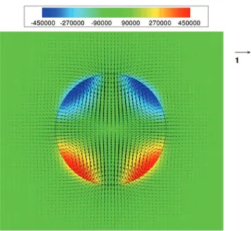
Snapshots of the interface location and vorticity are shown in Fig. 3and Fig. 4for Reosc

=

20 and Reosc

=

200,

respec-tively. It is clear from these figures that the vorticity is localized inside the bubble, whereas the flow remains potential outside.Forashape-oscillatingbubble,boththefrequencyandthedampingratearemainlycontrolledbythepotentialflow in the liquid phase. The asymptotic development of the damping rate given by Miller and Scriven [17] shows that, for a

Fig. 3.Velocity field, interface location and vorticity field (s−1_{) of an oscillating bubble at Re}

osc=20 (grid 256×512) using the GFCM.

Fig. 4.Velocity field (m s−1_{), interface location and vorticity field (s}−1_{) of an oscillating bubble at Re}

osc=200 (grid 256×512) using the GFCM.

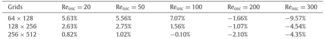
Table 8

Erroronthedampingrateβ2foranoscillatingbubblewithdifferentcomputationalgridswiththeexplicitGFCM.

Grids Reosc=20 Reosc=50 Reosc=100 Reosc=200 Reosc=300

64×128 1.49% 1.47% 9.75% 23.16% 41.72%

128×256 −0.20% 0.32% 1.99% 7.30% 13.71%

256×512 −0.31% 0.08% 0.70% 2.55% 5.36%

range of Reosc, i.e. between 20and 300. The restof the viscous dissipation comes fromthe potential flow in the liquid

phase.

For each Reynolds number of oscillation, a test has been computed with four different numerical methods (GFCM, explicit GFSCM, GFPM and DFM) and for three different mesh grids

(

64

×

128

)

,

(

128

×

256

)

and

(

256

×

512

)

, which describe a bubble

diameterwith32,64and128meshpoints,respectively.TheresultsofthesimulationsaresummarizedinTables 8,9,10 and 11, where the deviation of the numerical simulations relative to the theoretical predictions have been reported. The error