HAL Id: hal-02964970
https://hal.archives-ouvertes.fr/hal-02964970
Submitted on 12 Oct 2020
HAL is a multi-disciplinary open access
archive for the deposit and dissemination of
sci-entific research documents, whether they are
pub-lished or not. The documents may come from
teaching and research institutions in France or
abroad, or from public or private research centers.
L’archive ouverte pluridisciplinaire HAL, est
destinée au dépôt et à la diffusion de documents
scientifiques de niveau recherche, publiés ou non,
émanant des établissements d’enseignement et de
recherche français ou étrangers, des laboratoires
publics ou privés.
Energy-aware scheduling of malleable HPC applications
using a Particle Swarm optimised greedy algorithm
Nesryne Mejri, Briag Dupont, Georges da Costa
To cite this version:
Nesryne Mejri, Briag Dupont, Georges da Costa. Energy-aware scheduling of malleable HPC
applica-tions using a Particle Swarm optimised greedy algorithm. Sustainable Computing : Informatics and
Systems, Elsevier, 2020, 28, pp.100447. �10.1016/j.suscom.2020.100447�. �hal-02964970�
Energy-aware scheduling of malleable HPC applications using a Particle Swarm
optimised greedy algorithm
Nesryne Mejri
University of Luxembourg, Luxembourg
Briag Dupont
University of Luxembourg, Luxembourg
Georges Da Costa
IRIT Laboratory, University of Toulouse, France
Abstract
The scheduling of parallel tasks is a topic that has received a lot of attention in recent years, in particular, due to the development of larger HPC clusters. It is regarded as an interesting problem because when combined with performant hardware, it ensures fast and efficient computing. However, it comes with a cost. The growing number of HPC clusters entails a greater global energy consumption which has a clear negative environmental impact. A green solution is thus required to find a compromise between energy-saving and high-performance computing within those clusters. In this paper, we evaluate the use of malleable jobs and idle servers powering off as a way to reduce both jobs mean stretch time and servers average power consumption. Malleable jobs have the particularity that the number of allocated servers can be changed during runtime. We present an energy-aware greedy algorithm with Particle Swarm Optimized parameters as a possible solution to schedule malleable jobs. An in-depth evaluation of the approach is then outlined using results from a simulator that was developed to handle malleable jobs. The results show that the use of malleable tasks can lead to an improved performance in terms of power consumption. We believe that our results open the door for further investigations on using malleable jobs models coupled with the energy-saving aspect.
Keywords: Energy Efficiency, Malleable jobs, Particle Swarm Optimization, High Performance Computing, Scheduling
1. Introduction
The current world is massively abundant with valuable data. This by itself represents a reason -among others-for the increasing number of High-Perothers-formance Comput-ing (HPC) clusters, data centers, and cloud computComput-ing ser-vices seen in the past few years. This need for constantly processing enormous loads of data requires not only phys-ical means but also software actors capable of using the hardware capabilities to its fullest. These actors should act in an objective-oriented way when handling data. This is a scheduling problem that is not considered new, neither in applied fields nor in research. Indeed it has been a hot topic for years since it touches various domains such as in-dustrial processes, manufacturing, computing and trans-portation planning. In most of these applications, it is mainly concerned with how to dispatch a set of process-able resources over a finite set of processing resources, in a way that optimizes one or several objectives. Unsurpris-ingly it is the topic of this paper as there is a growing interest in parallel and distributed computing where it is critical to ensure a smooth execution for the distributed
applications. Another related matter that rises is energy efficiency, as more HPC clusters and data centers increase the CO2emission rate. As a matter of fact [1] states that digital technologies account for between 2.5% to 3.7% of the global greenhouse gas emissions. Data centres rep-resent 19% of the total energy required for the produc-tion and use of digital devices. The energy consumed by data centres is expected to increase by about 4% per year. Clearly reducing the energy consumption should be a goal and this issue should be approached from different angles. Moreover it has been shown that servers account for up to 75% of a data center energy consumption[2], and within this value, 50% can be due to idle servers [3]. The total energy consumed is not the only issue, the rate at which energy is consumed (power) must also be considered as it is bounded. For example the US Department of Energy EISC (Exascale Initiative Steering Committee) has set 20 MW as the upper limit for a buildable exascale system [4].
The energy saving problem can be solved from different perspectives, such as the hardware one or the software one. From the software part, a scheduler implementation can play a key role in the energy consumption of a data centre.
Usually, there are two main requirements to consider when building a scheduler; fairness and energy consumption. A scheduler is fair when it guarantees that every submitted job has a chance to be executed within a reasonable time. This is known as fair-share mechanisms [5].
Hence, the combined cost of a fair, performant and energy-efficient scheduler should be optimised to achieve an efficient use of servers and a lower energy and power consumption within data centers and HPC clusters. In the following section, a brief review of the literature is made. Next, the optimization problem is formally pre-sented by outlining the objectives and the performance criteria. Afterward, the used approach is thoroughly ex-plained along with the adopted assumptions and the op-timisation process. Following, the experimental setup is described. Lastly, the experimental results are presented and discussed.
2. Literature Review
Since scheduling parallel jobs is an NP-Hard problem [6] no known algorithm can solve it in polynomial time, and only approximations can be used to find near-optimal solutions. Consequently, the matter has been approached from different perspectives and setups depending on the used scheduling algorithm and the nature of the tasks to perform. Trystram-Mouni´e et al. [7] described approxima-tions for algorithms taking into account diverse paradigms of jobs; rigid ones, moldable ones, and malleable ones, an-alyzing and comparing the theoretical performance of each paradigm. Rigid jobs have a fixed number of required re-sources that cannot be changed once a job has been sched-uled. Furthermore, if this number is greater than the num-ber of available resources, the job may not be scheduled. Similarly, for moldable jobs, the number of required re-sources cannot be changed during runtime. However, the number of resources to allocate is defined by the scheduler before the job starts its execution. Lastly, malleable jobs are the most flexible ones since they behave like moldable jobs with the exception that the scheduler can adapt the number of their required resources even during execution [8]. For malleable jobs, the process of changing the number of required resources at runtime is called a reconfiguration. An example depicting malleable jobs and rigid jobs can be seen in Figure 1.
Figure 1: Scheduling of moldable jobs (left, middle) and of malleable jobs (right) (from [8])
An approach from literature [9] uses the malleable jobs paradigm because of its flexibility and efficiency. However,
assumptions are made about the homogeneity of the clus-ter, and PTGs (Parallel Task Graphs or Directed Acyclic Graphs) are considered as perfect malleable tasks. These assumptions do not reflect real-life setups. In reality, mal-leable jobs cannot be perfect, and their reconfiguration necessarily induces overheads such as communication be-tween nodes and time for data to be transferred. An-other work [10] addressing cloud computing services fo-cuses more on the optimisation aspect of providing high QoS and the improvement of energy consumption. It also provides a comparison of the Mixed Integer Linear Pro-gramming (MILP) approach against the Genetic Algorithm approach for the same objectives.
Finally, cutting-edge simulators such as Batsim [11] or SimGrid[12] do not support the scheduling of malleable jobs. Consequently, researchers are restricted from exper-imentally investigating potential improvements of perfor-mance offered by this paradigm.
3. Formulation of the problem
This section formally introduces the optimization prob-lem, that is given a set of malleable jobs, the goal is to find a scheduling strategy that optimizes the performance and the power consumption by respectively using job re-configurations and turning off idle servers. We define the following useful notions:
• A job is a set of identical parallel tasks submitted at the same time and that can be run on n distinct servers.
• The submission time is the time at which a job enters the queue of the scheduler.
• The speed-up factor α, is a real number between 0.5 and 1 indicating how parallelisable the computations within a job are.
• The mass corresponds to execution time of the job if it were to be run on a single server. In a rigid job context, the mass is directly related to the required time to complete the job, as it would be run over a fixed number of servers.
• The makespan is the time needed to complete a job once it starts executing. In a malleable job context, the completion time of a job also depends on factors such as the number of used servers n, the speed-up factor α and whether the job has been reconfigured. For a constant number of servers n it is defined sim-ilarly as in [13]:
makespan = mass nα
• The data D is the amount of data to transfer from n to m servers in case a reconfiguration takes place.
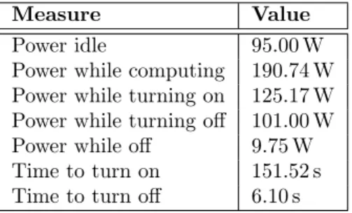
Measure Value Power idle 95.00 W Power while computing 190.74 W Power while turning on 125.17 W Power while turning off 101.00 W Power while off 9.75 W Time to turn on 151.52 s Time to turn off 6.10 s
Table 1: Reference values for servers power consump-tion
• The reconfiguration time Tn→m is the time needed to transfer data from n to m servers. It is given by:
Tn→m= (D n(d n me − 1) if n ≥ m D m(d m ne − 1) if n ≤ m 3.1. Criteria
The goal of this study is to reduce the average rate of energy consumption or power without compromising the fairness of the scheduler.
Classically, the objective of the scheduler is to minimise either the total makespan (the time to complete all the given jobs) or the mean or maximum stretch time. Due to the distributed aspect of the problem, the stretch time is potentially a more beneficial metric than the makespan, as it takes into account the time a job spends waiting in the queue. In a rigid job context, the stretch time is defined as the ratio of the difference between the termination time and the submission time to the actual job execution time. As outlined earlier, the execution time of malleable jobs can vary as it depends on the number of used servers as well as whether the job has been reconfigured. So the definition of the stretch time is adapted to:
stretch time =termination time − submission time mass
The other criterion to take into account is the power con-sumption of all the servers. Realistic energy concon-sumption approximations of the different server states were used in this study and are shown in Table 1. These values cor-respond to measurements made on the Tarus Grid’5000 cluster which was composed of 16 Dell PowerEdge R720 nodes each with two Intel Xeon E5-2630 [14]. It can be easily shown that saving energy by turning off a server is only profitable when the shutdown duration is of at least 260 s. This implies that a cycle of turning off, staying off for the minimum span of 260 s, and restarting a server lasts for about 362 s. In the model, the minimum allowed duration for a power-off is 362 s.
As a second metric, the normalized mean power con-sumption is considered. It is defined as the mean power consumption divided by the power consumption of an idle
server.
normalised mean power = mean power idle server power 3.2. Objective
Under the following scheduling constraints:
• A job must eventually be scheduled and completed. • No two jobs can be scheduled at the same time on
the same servers.
• A job can only be scheduled or reconfigured on servers that are powered on and idle.
The goal is to minimise the combined cost of the mean stretch time and the normalized mean power consumption. Therefore the objective function can be formalized as an energy-delay-product (EDP), which is a metric that had been used in [15], and that expresses the trade-off between the performance and the power consumption of our model. Thus the objective function is expressed as:
Minimise: mean stretch time × normalized mean power
4. Optimisation strategy
This section presents the adopted approach for min-imising the objective function under the previously men-tioned constraints.
4.1. Assumptions
The following assumptions were made when implement-ing the simulation environment supportimplement-ing malleable jobs. • The user submits a job request and the scheduler
handles it.
• The attributes of a job request are the submission time, the speed-up factor α, the mass, the minimum and the maximum number of servers required to run the job. All these parameters are considered known to the scheduler.
• The data amount D of a job can be queried by the scheduler at any time. This is a reasonable assump-tion as in reality, it should be possible to know how much data a program is using at a given time. • There is an upper limit Dmaxto the amount of data
a job can have, and this limit is known to the sched-uler.
• The scheduler has no knowledge about any future states, it only knows about the current and past states.
• The mass submitted by the user is only an estimate. Hence, the scheduler cannot use it to make exact predictions about the termination time.
4.2. Greedy Algorithm
Adding job reconfigurations and server power-offs to the capabilities of the scheduler increases the complexity of the scheduling problem. Therefore the selected approach to tackling the problem is to implement a greedy algorithm and use a meta-heuristic to tune its parameters.
Greedy algorithms are heuristic-based algorithms that always take the best immediate, or local, solution while finding an answer. Greedy algorithms find the overall or globally optimal solution for some optimization prob-lems but may find less-than-optimal solutions for some in-stances of other problems [16]. The implementation steps are described in Algorithm 1.
Algorithm 1: Greedy algorithm Input: A set of job requests
Output: A greedy scheduling with statistics servers available ← list of idle servers at time t active jobs ← list of running jobs at time t j by mass ← empty list
while queue and servers available do FIFO schedule(queued jobs) end
if servers available then j by mass ←
sort by biggest mass left(active jobs) while j by mass and servers available do
if reconfig decision then
attempt reconfiguation(j by mass) end
end end
if queue is empty and servers available then if shutdown decision then
shutdown(servers available, some duration) end
end
The scheduler’s implementation is based on three main parts. The first one prioritises the scheduling of the jobs in the queue per order of time submission. Once the queue is empty and there are still some idle servers, the sched-uler will try to reconfigure the running jobs by prioritis-ing the ones with the highest remainprioritis-ing mass. The third part takes place when the queue is empty, and there is no possibility of reconfiguring any of the running jobs, at that moment, the scheduler will shut down the unused servers. Again the scheduler’s main challenge is that it has no knowledge about the submission time of the upcoming jobs nor their parameters. Consequently, it cannot esti-mate in advance whether a reconfiguration would actually improve the performance as the servers that will be used for the reconfiguration may be required at any time for a new job. For a similar reason, shutting down idle servers may not always improve power consumption. Hence, in the next two sections, an explanation of the decision processes
mentioned as reconfig decision and shutdown decision in Algorithm 1 is presented.
4.2.1. Handling Reconfigurations
Finding a good representation of the decision-making process of the reconfigurations is not a trivial problem. Therefore, three inequalities are introduced as candidates to model the condition at which a reconfiguration should take place. The first condition is considered the most ba-sic one. It takes into account the main factors that are as-sumed to directly impact the outcome of reconfiguration: that is the number of used servers and the speed-up factor α of the job. It is also considered as the least complex as it introduces only three parameters. It is used later in the report within the setup Swarm1. The common attributes to the three conditions are: nnewwhich is the new number of servers that a job would be running on after a recon-figuration, nmax is the maximum number of servers a job can be assigned to (specified in the job request), and the speed-up factor α. Consequently, the condition1 is met if:
(nnew nmax)
wn× αwα× sreconf ig > 0.5
where wn is a weight between 0 and 1 and that is given to the ratio nnew
nmax. The speed-up factor α also carries a
weight wα. sreconf ig is a scaling factor between 0 and 1. The second condition is paired with the setup Swarm2. It is slightly more complex as it introduces an extra parame-ter wD that needs to be tuned. The idea is that since the duration of a reconfiguration is impacted by the amount of data to transfer between the servers, it would be fair to embed such amount in the decision-making process. In that way, a reconfiguration takes place if the following con-dition2 is met if:
(nnew nmax
)wn× αwα× ( D
Dmax
)wd× sreconf ig > 0.5
where D is the amount of data of the job, and Dmaxis the maximum amount of data any job can have. This ratio carries a weight wD ranging from 0 to 1, and that should be also tuned.
Finally condition3 introduces a bias term instead of the scaling factor sreconf ig which is in the range of -0.5 and 0.5. It also relies on the tanh function and the previously mentioned parameters to decide whether a reconfiguration should be performed. It is used in the setup Swarm3, and is met if: tanh((nnew nmax) wn× αwα× ( D Dmax) wd+ bias) > 0.5
For condition1 and condition2, the value of 0.5 in each of the conditions is arbitrary, other values were tested and it did not seem to affect significantly the results. For con-dition3, 0.5 was chosen over 0 to push the decision pro-cess towards using reconfigurations more often as the tanh function is not symmetrical around 0.5.
4.2.2. Handling Power-offs
For power-offs, it is assumed that the main factor that affects whether it is beneficial to shut down the idle servers is the ratio of available servers to the total number of servers. This decision, referred to as shutdown decision in Algorithm 1, is based on the following condition:
(nav ntot)
wof f × sof f > 0.5
where nav is the number of available servers, ntotthe total number of servers, wof f a weight between 0 and 1 that re-flects the importance of this ratio when making the shut-down decision and sof f is a scaling factor on the previ-ous ratio. Additionally, instead of always powering off the servers for the same constant amount of time, two differ-ent shutdown durations are proposed; t1 of f and t2 of f. Indeed, the scheduler does not know in advance whether the shutdown will be beneficial, so a probability pt1 of f for
choosing t1 of f over t2 of f is introduced. 4.2.3. Greedy algorithm parameters
The decision process is thus influenced by the combi-nation of the previously mentioned parameters from the shutdown process and the chosen condition of the job re-configuration. The weights and scaling factors range be-tween 0 and 1. The bias term range is bebe-tween -0.5 and 0.5. The powering off times are only constrained by the 362 seconds value that is the minimum duration that guar-antees energy saving. Thus during the optimization pro-cess, either eight or nine parameters need to be tuned. A summary of these parameters can be found in Table 2. Ad-ditionally, it is worth mentioning that when tests were run, it was more challenging to find a condition that models the decision-making process of the reconfigurations than find-ing a condition modellfind-ing power-offs. The latter condition seemed to be effective, as it explicitly uses the ratio of idle servers to the total number of servers.
The next step is to find the combination of parameter values that minimises the objective function. Since they are continuous and relatively numerous, the search space is very large. Thus to explore it and find an optimal so-lution a meta-heuristic algorithm, namely Particle Swarm Optimisation (PSO), is used.
4.3. Particle swarm optimization
As mentioned in the previous section, the goal of the particle swarm optimization (PSO) is not to directly find an optimal solution to schedule the different jobs but rather to find an optimal set of parameters that could improve the decision processes of the greedy algorithm.
PSO is a nature-inspired algorithm that imitates the behaviour of animal flocks. A Swarm is a group of particles which are mobile entities characterised by their position, velocity and cost. A swarm converges towards an ideal location as its individuals move with respect to the group best-known position and their respective best-known po-sition. This technique enables for an exploration of the
Overall reconfiguration parameters wn wα sreconf ig wD bias Servers count weight Speedup factor α weight Scaling factor Data weight Bias term Power off parameters
wof f sof f t1of f t2of f pt1off Available servers count weight Scaling factor Duration 1 Duration 2 t1of f proba-bility
Table 2: Overall parameters of the greedy algorithm
search space while converging towards an optimal solution [17]. The used algorithm is similar to the one described in [18]. It uses the reflect method to deal with boundary escape from [19]. The used PSO algorithm is outlined in Algorithm 2.
Algorithm 2: PSO algorithm
Initialise population position vectors ( ~xi) randomly
for number of steps do
for i=1 to Population Size do ~
vi= χ(~vi+ φ1( ~pi− ~xi) + φ2( ~pg− ~xi)) ~
xi= ~xi+ ~vi
if f ( ~xi) < f ( ~pi) then ~
pi= ~xi end
handle boundaries() end
for i=1 to Population Size do if f ( ~xi) < f ( ~pg) then ~ pg= ~xi end end end
In our experiments, the set of parameters is either rep-resented as an 8-dimensional vector or a 9-dimensional vector. ~xi depicts the position of the ith particle. Each particle has a velocity vector ~vi, used to update the vector
~
xi, at every step. ~vi is calculated using:
~
vi= χ(~vi+ φ1( ~pi− ~xi) + φ2( ~pg− ~xi))
where χ is a constant influencing the magnitude of update. It was found that a value of 0.1 works well compared to higher values that tend to push particles out of bounds too quickly. ~pi is the particle best-known position, ~pg is the global best position. φ1 and φ2 are random numbers between 0 and 2 generated for each particle at each time step. The cost function f for a particular configuration is a function mapping a position vector to a real number.
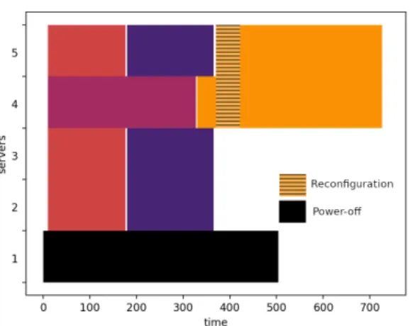
Figure 2: Visual output from the simulator
As for boundary escape, if a parameter j of ~xi goes below or above the xj min/max thresholds then it is handled as follows:
xij= xjmax− (xij− xjmax) if xij > xjmax xij= xjmin+ (xjmin− xij) if xij < xjmin
5. Experimental setup 5.1. Simulation environment
As there are no known simulators -to our knowledge-supporting the scheduling of malleable jobs, a simulation environment was developed using python to test the per-formance of the designed scheduling strategy. At the time of writing this paper, it only provided reconfiguration of jobs from a smaller to a larger number of servers as it was thought to be more relevant in decreasing the mean stretch time. An example of the visualisation output of the simulator can be seen in Figure 2.
5.2. Jobs Generation
To simulate a realistic environment, Google data centres-like jobs were generated similar to [20]. The only difference lies in the way a job is defined. In [20] jobs are sets of small sequential tasks schedulable in a particular order. In our approach, a job is a single parallelisable task. A uniform random distribution is used to generate parameters such as the speed-up factors, the data and the required number of servers. All the undertaken experiments generated 50 jobs to be scheduled on ten servers. A summary of the job generation parameters is shown in Table 3 where the dy-namism is the average duration between two consecutive jobs and the disparity is the ratio of the average makespan to the median makespan. The values for the mass and dis-parity correspond to the average values obtained in [20].
Parameter Used value
Server count 10 Job count 50 Dynamism 500 Mass 1700 Disparity 3.8 speed-up factor (α) U (0.5, 1) Data U (10, 500)
Table 3: Parameters used for the generation of jobs
5.3. Particle Swarm search of parameters
Since the number of parameters to tune is based on which condition is used for reconfiguration, three differ-ent swarms of 30 particles each were trained. Swarm1 (training), Swarm2 (training) and Swarm3 (training) use respectively condition1, condition2 and condition3. Each particle of each trained swarm was assigned set of valid parameters following the laws described in [20] and the values in Table 3. At each epoch k a set Gk is generated, where Gk = {S1, S2, .., S50} and Si is a set of 50 different jobs. Every particle had to schedule Gk independently. This partitioning of the set of jobs Gkinto smaller subsets Si is used to prevent the parameters within particles from overfitting a particular set of jobs. It also ensures that the job generator is updated with newer seeds guaranteeing diversity among the jobs. The scheduling of one set Si is further referred to as an experiment. The cost function is evaluated for each particle, by taking the average cost of the 50 Siwithin Gk. Also, every set of generated jobs Gk at epoch k is different from the one generated at epoch k + 1. The total number of used epochs is 100. This value was chosen as it was noticed that all particles had con-verged towards the same set of parameters and there was little change from one epoch to the next.
The mean cost of all the particles as a function of the number of epochs for each trained swarm is depicted in Figure 3.
The graph shows that for each of the swarms, the pa-rameter search went through three different phases. From epoch one to about 20, there is a clear improvement in min-imizing the cost function. Then from epoch 20 to about 70, particles still have quite different sets of parameters. Yet, these parameters tend to get closer to one another. At this point, the swarm is exploring the neighbourhood of the minimum it would later settle in, which justifies the flattening of the cost values from about epoch 40 to 70. From epoch 70 to 100, the mean cost slowly decreases until convergence, and the swarm finds a minimum optimising the cost function. So the three trained swarm converged at around the same range of epochs. Moreover, those sim-ilarities in the cost pattern can be explained by the fact that the training took place under the same seed and that the job generator had not been modified, which resulted in having the same job distribution for each of the swarms.
Figure 3: Mean cost of all the particles against the number of epochs during training
Reconfiguration parameters
Swarm1 Swarm2 Swarm3
wn 0.175 0.348 0.529
wα 0.742 0.833 0.645 sreconf ig 0.331 0.579 N/A
wD N/A 0.730 0.289
bias N/A N/A -0.106
Power off parameters
Swarm1 Swarm2 Swarm3 wof f 0.455 0.516 0.494
sof f 0.760 0.814 0.813
t1 of f 899 528 632
t2 of f 1405 2962 1233 pt1 of f 0.717 0.959 0.615
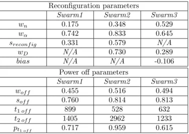
Table 4: Configuration of parameters found by PSO of each of the trained swarms
This shows that the performance of the scheduler is highly dependent on the set of jobs to be scheduled. The found parameters are shown in Table 4.
The implication of the found results will be discussed in more details in the next section. Nevertheless, it is already worth noting that even though every particle’s parameters are initialised randomly, every trained swarm learned two different shutdown time durations a short one for t1of f and
a long one for t2of f, and whenever a power-off takes place at least 60% of the times, it lasts for a shorter amount of time. The difference in values for the shutdown times found by Swarm2 is quite large. In fact t1 of f is close to the minimum required duration for energy-saving whereas t2 of f is more than twice as large as the values found by Swarm1 and Swarm3. However the probability for choos-ing t1 of f over t2 of f in Swarm2 is about 96%, meaning that longer shutdown times will be rare. No indication was given in the initial values of the particles that one time should be longer than the other.
5.4. Comparison setups
To evaluate the performance of the scheduler, ten dif-ferent experimental setups are introduced and run under identical conditions. In each of these setups, jobs are gen-erated such there is only one big set of sets of jobs G1that is composed of 100 subsets Si, and where each Si contains 50 different jobs to be scheduled on ten identical servers. The main distinction between the first four setups and the last six lies within the decision-making process, which is based on the parameters defined in Table 2. In the first four setups, the reconfigurations and power-offs are per-formed whenever possible without any involvement of the parameters. Whereas the last six setups rely on those pa-rameters to make a decision.
• FIFO (FIFO): The base case. It is only the first step of the greedy algorithm, a naive FIFO sched-uler where the jobs are scheduled according to their submission time.
• FIFO & Reconfigurations (FIFO-Rcfg): A FIFO sched-uler that always reconfigures jobs whenever servers are available.
• FIFO & Power off (FIFO-Poff ): A FIFO scheduler that always shuts down idle servers -when possible-for a constant downtime of 900 seconds.
• FIFO & Reconfigurations & Power off (FIFO-Rcfg-Poff ): A FIFO scheduler combining reconfigurations and power-offs in the same fashion as in FIFO-Poff and FIFO-Rcfg.
• Random parameters (Rand-Param1 ): A FIFO sched-uler that uses condition1 to reconfigure jobs and shuts down idle servers based on randomly gener-ated parameters.
• Random parameters (Rand-Param2 ): A FIFO sched-uler that uses condition2 to reconfigure jobs and shuts down idle servers based on randomly gener-ated parameters.
• Random parameters (Rand-Param3 ): A FIFO sched-uler that uses condition3 to reconfigure jobs and shuts down idle servers based on randomly gener-ated parameters.
• With Swarm1 parameters (Swarm1 ): A FIFO sched-uler that uses condition1 and that is capable of re-configuring jobs and shutting down servers based on the PSO parameters found by Swarm1 (training). • With Swarm2 parameters (Swarm2 ): A FIFO
sched-uler that uses condition2 and that is capable of re-configuring jobs and shutting down servers based on the PSO parameters found by Swarm2 (training). • With Swarm3 parameters (Swarm3 ): A FIFO
sched-uler that uses condition3 and that is capable of re-configuring jobs and shutting down servers based on the PSO parameters found by Swarm3 (training).
6. Results
In this section, the method used for ranking the differ-ent setups is outlined. The results of the experimdiffer-ents are analysed by first looking at the number of power-offs and reconfigurations performed by each setup. Then, the indi-vidual components of the cost are investigated. Following, a statistical analysis of the overall costs is performed. Fi-nally a resilience test on the best performing setup along with a scale-up test are presented.
6.1. Ranking methodology
To draw conclusions from the results, a ranking be-tween each of the setups is established. In this section, the statistical method for the ranking is described. The first step of the approach is to rank each setup for each sched-uled set of jobs. A rank of 1 denotes the best performing setup (lowest mean cost) and a rank of 10 the worst per-forming one. As one hundred sets Siof jobs were used for the experiment, one hundred rankings are obtained. Then, the average ranking of each setup is calculated. To evalu-ate whether those average ranks are significantly different from the mean rank (5.5), the Friedman χ2
F and its corre-sponding p − value are used. Thus for a confidence level of 95% corresponding to an α value of 0.05, it is mean-ingful to perform post-hoc tests as described in [21] if the p − value is less than 0.05. The post-hoc tests make it pos-sible to identify significant pairwise differences among the different setups. This is done by first finding the standard error (SE) between two setups using:
SE = r k(k + 1) 6N = r 10 × 11 6 × 100 = 0.265
where k is the setup count and N the number of exper-iments. Using the average ranks and the standard error the z − values are computed using:
z = Ri− Rj SE
where Riand Rj are the average ranks of two different setups. From the z − values, the corresponding probabili-ties (p − values) are found. The null hypothesis is that the difference in ranks is due to chance. However, if a p−value is below α = 0.05, then the null hypothesis can be rejected with level of confidence of 95%.
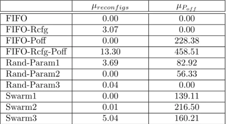
6.2. Reconfigurations and Power-offs results
Table 5 shows the average number of reconfigurations and the average number of power-offs per setup. The most striking result is that the average number of reconfigura-tions performed by the setup Swarm1 is zero. This implies that the parameters do not allow for any reconfigurations to take place for the generated jobs. The parameters from Swarm2 allow for very few reconfigurations to take place. This is also an unexpected result as one would expect that
µreconf igs µPof f FIFO 0.00 0.00 FIFO-Rcfg 3.07 0.00 FIFO-Poff 0.00 228.38 FIFO-Rcfg-Poff 13.30 458.51 Rand-Param1 3.69 82.92 Rand-Param2 0.00 56.33 Rand-Param3 0.04 0.00 Swarm1 0.00 139.11 Swarm2 0.01 216.50 Swarm3 5.04 160.21
Table 5: Average number of reconfigurations and
power-offs of each setup
reconfigurations could improve the average stretch time. This result seems to highlight the difficulty of deciding when to perform reconfigurations and that if they are not carefully undertaken the performance might not improve. The average number of reconfigurations made by the three setups Rand-Param show that the improved cost reached by the Swarm setups is due to the optimization process and not just the choice of the equation describing the de-cision process. The average numbers of power-offs for the three Swarm setups are of the same order of magnitude which can be explained by the fact that the equations and parameters governing the power-off decision process for those three setups are the same. The different Swarm based set-ups allow for a relatively large number of power-offs. It may seem that this could cause power spikes and have a negative impact on the energy saved. However mod-ern hardware can slightly shift the time of powering dif-ferent servers on and off so that they do not all take place at the same time and therefore avoiding power spikes.
6.3. Ranking by the mean stretch time
Figure 4 shows the distributions of the mean stretch time metric obtained from conducting 100 experiments for each of the different setups. Although it cannot be seen on the graphs, the setup FIFO-Rfcg-Poff has a maximum mean stretch time (around 80) that is much higher than in any of the other setups. The distribution from FIFO-Poff also suggests that mean stretch time was higher than for the other setups in some instances. The distributions of the mean stretch times of the setups using the decision equations seem to have similar shapes for random param-eters and PSO-obtained paramparam-eters. Another setup pair with similar distributions corresponds to FIFO and FIFO-Rcfg. This is not surprising as the logic between these two setups is quite similar. Using the statistical methodology previously described, the Friedman χ2
F is found to be equal to 442.05 which corresponds to a p − value of 1.43 × 10−89 which signifies that it is meaningful to perform post-hoc tests to identify significant pairwise differences. The rank-ing obtained with a confidence level of 95% is shown in
Rank Setup
1 Swarm2
2 Swarm3 and Swarm1
3 FIFO and Rand-Param1 and Rand-Param3 4 FIFO-Rcfg and Rand-Param2 5 FIFO-Rcfg-Poff and FIFO-Poff
Table 6: Setups ranking by the mean stretch time
Rank Setup
1 FIFO-Poff and Swarm1 2 Swarm2 and Swarm3 3 FIFO-Rcfg-Poff and Rand-Param2
4 Rand-Param1
5 FIFO and Rand-Param3
6 FIFO-Rcfg
Table 7: Setups ranking by the mean normalised power
Table 6. Clearly, the setups using the PSO-obtained pa-rameters ranked better than the other setups. The setups with the worst performances are Poff and FIFO-Rcfg-Poff. This result can be explained by the fact that if the power-offs are not scheduled properly then the mean stretch time increases as the servers may be off at times when there is high demand.
6.4. Ranking by the mean normalized power consumption Similarly to the previous section, Figure 5 shows the different distributions of the average normalised power met-ric of each setup. The range of values seems to vary over a smaller range from one setup to another compared to the stretch times shown in the previous section. This is expected as power is a measure of the rate of energy trans-formation, and there is a narrower range of allowed val-ues (with respect to the states of the servers) at a given time. Unsurprisingly the setups that do not allow perform-ing power-offs have a higher minimum average normalised power. The Friedman χ2F is found to be equal to 831.72 which corresponds to a p − value of 3.15 × 10−173 which signifies that it is meaningful to perform post-hoc tests to identify significant pairwise differences. The ranking ob-tained with a confidence level of 95% is shown in Table 7. As expected, the FIFO-Poff setup that allows performing power-offs whenever possible ranks best on this metric. The setups that did not allow for any power-offs rank last. Again the three Swarm setups rank among the best ones.
6.5. Ranking by the overall cost
In this section the obtained cost values are compared to identify which setup may lead to a better overall perfor-mance. As a reminder, the cost function is defined as the product of the mean stretch time and the mean normalised power.
Figure 4: Histograms of the mean stretch time of each setup
Figure 5: Histograms of the mean normalised power of each setup
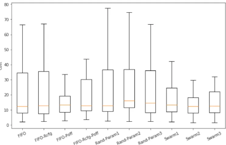
Figure 6: Boxplots of the cost of each setup
Figure 7: Heatmap of the performance pairwise com-parisons between setups on the cost criterion
Figure 6 shows the distribution of the overall cost val-ues obtained from conducting 100 experiments in each setup. It seems that the cost values of Swarm1, Swarm2 and Swarm3 are more skewed towards a lower cost than in the other setups.
Figure 7 shows pairwise comparisons of the number of times a particular setup obtained a lower cost value than an another setup. Clearly the three Swarm setups perform better than all the other setups on the majority of the experiments.
The average ranking over the 100 experiments can be seen in Table 8. It can be noted that no setup has an aver-age rank that is close to 1, meaning that there is probably no setup that outranks all the others on most occasions.
The Friedman χ2
F is in this case equal to 448.09 which corresponds to a p − value of 7.33 × 10−91. Thus for a con-fidence level of 95% corresponding to an α value of 0.05, it is meaningful to perform post-hoc tests to identify signifi-cant pairwise differences among the different setups. The
Setup Average ranking FIFO 5.49 FIFO-Rcfg 7.22 FIFO-Poff 7.58 FIFO-Rcfg-Poff 9.02 Rand-Param1 4.97 Rand-Param2 6.72 Rand-Param3 5.07 Swarm1 3.12 Swarm2 2.45 Swarm3 3.39
Table 8: Average ranking of each setup over the 100 experiments
Rank Setup
1 Swarm1 and Swarm2 and Swarm3 2 FIFO and Rand-Param1 and Rand-Param3 3 Rand-Param2 and FIFO-Rcfg and FIFO-Poff 4 FIFO-Rcfg-Poff
Table 9: Setups ranking by the overall cost
weak ranking among the six setups is shown in Table 9. The worst performing setup is FIFO-Rcfg-Poff. It im-plies that reconfigurations and power-offs require a care-ful decision-making process to ensure an increase in per-formance, and that it is not beneficial to perform them whenever it is possible. The three Swarm setups are all ranked first, which can be explained by the exploration of the parameter space that allowed the algorithms to ’learn’ to react to the job generator’s distribution. Interestingly, there is no statistical evidence that FIFO performs bet-ter than Rand-params1 or Rand-params3 as they are all ranked second. To evaluate the significance of this rank-ing, a resilience test is described in the next section.
6.6. Resilience of PSO parameters
To test the ability of the three Swarm setups to respond to changes in the job generator’s distribution, the setups were re-run under identical conditions to the ones in the previous section. The parameters of the job generator were slightly adjusted to simulate an environment where the frequency, the mass and the data of the jobs increased. Thus simulating an increase in the demand. The change of values can be found in Table 10.
Table 11 shows that this time the Swarm1, Swarm2, Rand-Param2 and Rand-Param3 allowed performing re-configurations. This shows that the decision process of reconfigurations is sensitive to the distribution of the jobs and that a slight change in the job’s parameters results in a different scheduling strategy.
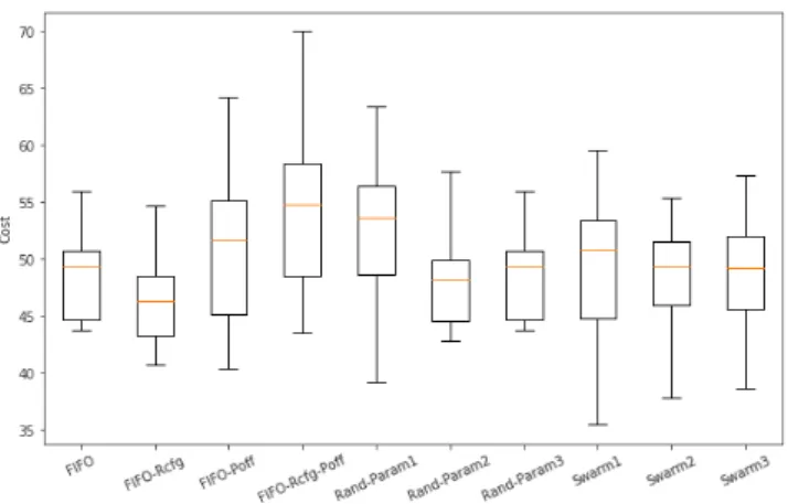
Figure 8 displays the different distributions of the costs. It can be seen that the setup FIFO-Poff that allows for
Parameter Previous Value New Value
Server count 10 10 Job count 50 50 Dynamism 500 300 Mass 1700 1900 Disparity 3.8 4.5 Speed-up factor α U (0.5, 1) U (0.5, 1) Data U (10, 500) U (10, 800)
Table 10: Jobs generator parameters used in the re-silience test µreconf igs µPof f FIFO 0.00 0.00 FIFO-Rcfg 4.34 0.00 FIFO-Poff 0.00 297.33 FIFO-Rcfg-Poff 5.77 189.25 Rand-Param1 2.92 20.27 Rand-Param2 3.63 11.19 Rand-Param3 2.50 0.00 Swarm1 7.53 87.32 Swarm2 1.23 184.27 Swarm3 4.85 128.89
Table 11: Average number of reconfigurations and
power-offs of each setup in the resilience test
power-offs to be performed whenever possible seems to have an overall cost distribution skewed towards lower val-ues. This can be explained by the fact that this setup is the one that performs the highest number of power-offs per set of jobs thus entailing a lower average power consumption. This does not necessarily imply that it is a beneficial setup as the mean stretch time can be very large. The Fried-man Chi-square value χ2F = 165.67 and its corresponding p − value (4.93 × 10⁻³¹) suggest that post-hoc testing can be meaningful. This time the ranking cannot be as clearly established as in the previous section and the weak rank-ing displayed in Table 12 was produced usrank-ing a confidence level of 90%. This time again Swarm2 ranks first. How-ever, the other two setups Swarm1 and Swarm3 did not perform as well as they rank third. It is worth mention-ing that the simple FIFO scheduler that performs neither reconfigurations nor power-offs ranks second. Unsurpris-ingly using random parameters for the decision processes leads to a poor overall performance.
6.7. Scale up test
The scale-up test aims at simulating a more realistic environment by increasing the number of servers from 10 to 100 while keeping the average number of submitted jobs per server per unit time the same as before. Similar to the resilience test, the goal is to test how the different setups would behave in an environment that is different from the
Figure 8: Cost of each used setup in the resilience test
Rank Setup
1 Swarm2
2 FIFO
3 Swarm3 and FIFO-Rcfg and Swarm1 and FIFO-Poff
4 FIFO-Rcfg-Poff and Rand-Param1 and Rand-Param3
5 Rand-Param2
Table 12: Setups ranking during the resilience test
one in which the optimization process took place. The change in the parameters made during the scale-up test can be found in Table 13.
As shown in Table 14, the average number of recon-figurations and power-offs performed by the three Swarm setups during the scale-up test are similar to the ones of the initial experiment. This shows if the jobs distribution is kept the same on a larger scale, the three Swarm setups behave consistently. However, this is not the case for the setups using random parameters, as Rand-Param2 that did not initially allow for reconfigurations, now performs a large average number of reconfigurations.
Figure 14 shows the cost distribution of the different setups. The three Swarm setups have a whisker in the
Parameter Previous
Value New Value
Server count 10 100 Job count 50 500 Dynamism 500 50 Mass 1700 1700 Disparity 3.8 3.8 Speed-up factor α U (0.5, 1) U (0.5, 1) Data U (10, 500) U (10, 500)
Table 13: Scale-up parameters
µreconf igs µPof f FIFO 0.00 0.00 FIFO-Rcfg 76.35 0.00 FIFO-Poff 0.00 266.17 FIFO-Rcfg-Poff 75.40 233.41 Rand-Param1 0.00 180.01 Rand-Param2 30.74 0.00 Rand-Param3 0.00 0.00 Swarm1 0.00 150.76 Swarm2 0.11 192.80 Swarm3 12.63 170.75
Table 14: Average number of reconfigurations and
power-offs during the scale-up test
Rank Setup
1 FIFO-Rcfg
2 Rand-Param2
3 Rand-Param3 and FIFO 4 Swarm1 and Swarm2 and Swarm3
5 FIFO-Poff
6 Rand-Param1
7 FIFO-Rcfg-Poff
Table 15: Setups ranking by overall cost in the scale-up test
lower costs that is longer than in Figure 6 and Figure 8. This implies that the lower quartiles spreads over a larger range of costs than in the previous two tests. There is some overlap of the different distributions and further analysis needs to be conducted to establish a ranking. The Fried-man Chi-square value χ2
F = 358.68 and its coresponding p − value (8.80 × 10−72) suggest that post-hoc testing can be meaningful. The weak ranking is shown in Table 15. The result is rather unexpected as the setup FIFO-Rcfg that allowed for reconfigurations to take place whenever possible ranks first. A large number of servers provides a larger number of possible ways to schedule a given job. A reconfiguration is less likely to have a large effect on the fractional number of servers being used if the number of servers is large. This result can also be explained by the fact that the setup FIFO-Rcfg performed really well under the mean stretch time metric, it did however perform very poorly on the average power metric. The different three Swarm setups ranked equally well at rank 4 despite a be-havior that is consistent with the initial test. When scaling up there does not seem to be a significant advantage in us-ing one of the decision equation over any of the other ones. The setup that allows for reconfigurations and power-offs to take place whenever possible ranks last similar to all the previous tests.
Figure 9: Cost of each used setup in the scale up test
6.8. Discussion of results and limitations
The results show that using a decision process for re-configurations and power-offs can lead to a low overall cost. This decision process is based on the scheduler state and made use of parameters that were tuned using PSO. How-ever, this performance was found to be sensitive to changes in the way jobs are submitted and the total number of servers in the HPC cluster. The difficulty with taking energy consumption as a metric is that minimising it by turning off servers can have a negative impact on the jobs waiting time in the queue. Therefore a setup that ranks well on one of the metrics does not necessarily rank well on the other. It would be interesting during the PSO train-ing to have variable weights over the metrics within the objective function. It would prevent that one metric gets favoured over the other. This was probably the case with the setups that did not allow for reconfigurations to take place. One of the limitations is that the PSO training can take a long time, especially if the number of servers and jobs are large. Our implementation could be improved by using multi-processing and generating jobs in advance so that they do not have to be re-generated every time a swarm has to be trained. This would increase the speed of experimentation with the proposed equations for the decision process. In this investigation, the job generator simulates a realistic distribution for the frequency at which jobs are submitted and their mass. But, both the speed-up factors and the data amount are drawn from uniform random distributions. Using a more realistic distribution for those parameters might improve the ability of the PSO to find patterns in the jobs. Finally, another aspect that is not taken into consideration in this investigation is that turning servers on and off frequently may affect their life-time. This is particularly important when considering the environmental aspect, as energy is not only required when the servers are used but also when they are manufactured and disposed of.
7. Conclusions & Perspectives
This paper presented a solution that aims at improving the performance of HPC schedulers by lowering both the mean stretch time and the average power consumption by relying on malleable job reconfigurations and server power-offs. As current simulators do not support the scheduling of malleable jobs, we implemented our own simulator. The job generator’s distribution was modelled based on real data. The proposed algorithm consisted of three steps: FIFO scheduling, reconfiguration attempts and powering off of the remaining idle servers. Various parameters and conditions were used to decide whether reconfigurations and power-offs should be performed. It was assumed that the scheduler has no knowledge about any future states and used only local context knowledge to make decisions. Three different equations were used to decide whether a reconfiguration should take place and the parameters of those equations were tuned using PSO. It was found that the three different setups using the PSO-obtained param-eters performed equally well and better than the other se-tups as long as the distribution of jobs is similar to the one it was trained on. If the frequency at which jobs are sub-mitted as well as their average masses are increased, one of the setups using PSO-obtained parameters ranks first with a level of confidence of 90%, but the other two did not perform so well. If the number of servers is increased to a more realistic number (100) then it was found that the setup that only used the FIFO scheduling as well as reconfigurations whenever possible performed best. How-ever, this performance was at the expense of the average power metric.
We believe that the malleable job paradigm should be investigated further by, for example, allowing jobs to be as-signed to a lower number of servers if the queue becomes too long. This would require keeping some statistics about the average length of the queue at a given time. Being able to accurately predict the remaining mass of a job at a given time would facilitate the evaluation of whether a reconfig-uration could be beneficial. Probably one of the biggest challenges remains to find a suitable encoding for mal-leable tasks so that other meta-heuristic algorithms could be used to find more optimal solutions.
8. Acknowledgment
The work presented in this paper has been funded by the ANR in the context of the project ENERGUMEN, ANR-18-CE25-0008.
We would like to thank Prof. Pascal Bouvry and Dr. Gr´egoire Danoy for their guidance throughout the project. We would also like to thank Luc Sinet for his invaluable advice on software development and Lucas Romao for his support.
References
[1] H. Ferreboeuf, Lean ict: Towards digital sobriety, Tech. rep., The Shift Project (2018).
[2] F. Pinel, J. Pecero, S. Khan, P. Bouvry, Energy-efficient scheduling on milliclusters with performance constraints, Pro-ceedings - 2011 IEEE/ACM International Conference on Green Computing and Communications, GreenCom 2011 (2011) 44– 49doi:10.1109/GreenCom.2011.16.
[3] V. Villebonnet, G. Da Costa, L. Lefevre, J.-M. Pierson, P. Stolf, Energy aware dynamic provisioning for heterogeneous data cen-ters (2016) 206–213doi:10.1109/SBAC-PAD.2016.34.
[4] J. Shalf, S. Dosanjh, J. Morrison, Exascale computing tech-nology challenges, in: High Performance Computing for Com-putational Science – VECPAR 2010, Springer Berlin Heidel-berg, Berlin, HeidelHeidel-berg, 2011, pp. 1–25. doi:10.1007/978-3-642-19328-6 1.
[5] A. Sedighi, Y. Deng, P. Zhang, Fairness of task schedul-ing in high performance computschedul-ing environments, Scalable Computing: Practice and Experience 15 (2014) 273–285. doi:10.12694/scpe.v15i3.1020.
[6] G. Rauchecker, G. Schryen, High-performance computing for scheduling decision support: A parallel depth-first search heuristic (12 2015).
[7] D. Trystram, G. Mouni´e, P.-F. Dutot, Scheduling parallel tasks: Approximation algorithms (2003) 1–40.
[8] J. Hungershofer, On the combined scheduling of malleable and rigid jobs, IEEE (2004). doi:https://doi.org/10.1109/SBAC-PAD.2004.27.
[9] H. Casanova, F. Desprez, F. Suter, Minimizing stretch and makespan of multiple parallel task graphs via malleable allo-cations (2010) 1–10doi:10.1109/ICPP.2010.16.
[10] T. Gu´erouta, Y. Gaouaa, C. Artiguesa, G. Da Costa, P. Lopeza, T. Monteila, Mixed integer linear program-ming for quality of service optimizationin clouds (2017) 1– 18doi:10.1016/j.future.2016.12.034.
[11] P.-F. Dutot, M. Mercier, M. Poquet, O. Richard, Batsim: A realistic language-independent resources and jobs management systems simulator (2017) 178–197doi:10.1007/978-3-319-61756-5 10.
[12] H. Casanova, A. Legrand, M. Quinson, Simgrid: A generic framework for large-scale distributed experiments, in: Tenth In-ternational Conference on Computer Modeling and Simulation (uksim 2008), IEEE, 2008, pp. 126–131.
[13] G. S. Prasanna, B. R. Musicus, Generalized multiprocessor scheduling and applications to matrix computations, IEEE Transactions on Parallel and Distributed systems 7 (6) (1996) 650–664.
[14] M. Poquet, Simulation approach for resource management, Data structures and algorithms [cs.ds], Universit´e Grenoble Alpes (2017).
[15] H. S. Azad, Advances in GPU Research and Practice, 1st Edi-tion, Morgan Kaufmann Publishers Inc., San Francisco, CA, USA, 2016.
[16] P. E. Black, greedy algorithm (2005).
URL https://www.nist.gov/dads/HTML/greedyalgo.html [17] D. Bratton, J. Kennedy, Defining a standard for particle swarm
optimization, in: 2007 IEEE Swarm Intelligence Symposium, 2007, pp. 120–127.
[18] M. Clerc, J. Kennedy, The particle swarm - explosion, stability, and convergence in a multidimensional complex space, IEEE Transactions on Evolutionary Computation 6 (1) (2002) 58–73. [19] S. Helwig, J. Branke, S. Mostaghim, Experimental analysis of bound handling techniques in particle swarm optimization, IEEE Transactions on Evolutionary Computation 17 (2013) 259 – 271. doi:10.1109/TEVC.2012.2189404.
[20] G. Da Costa, L. Grange, I. Courchelle, Modeling and generating large-scale google-like workload (2016) 1– 7doi:10.1109/IGCC.2016.7892623.
[21] S. Garc´ıa, F. Herrera, An extension on ”statistical comparisons of classifiers over multiple data sets” for all pairwise
compar-isons, Journal of Machine Learning Research - JMLR 9 (12 2008).
![Figure 1: Scheduling of moldable jobs (left, middle) and of malleable jobs (right) (from [8])](https://thumb-eu.123doks.com/thumbv2/123doknet/14427012.514414/3.892.59.441.956.1030/figure-scheduling-moldable-jobs-left-middle-malleable-right.webp)