A millennial multi-proxy reconstruction of summer PDSI for Southern South America

HAL Id: insu-00643480

https://hal-insu.archives-ouvertes.fr/insu-00643480

Submitted on 22 Nov 2011

HAL is a multi-disciplinary open access

archive for the deposit and dissemination of

sci-entific research documents, whether they are

pub-lished or not. The documents may come from

teaching and research institutions in France or

abroad, or from public or private research centers.

L’archive ouverte pluridisciplinaire HAL, est

destinée au dépôt et à la diffusion de documents

scientifiques de niveau recherche, publiés ou non,

émanant des établissements d’enseignement et de

recherche français ou étrangers, des laboratoires

publics ou privés.

PDSI for Southern South America

E. Boucher, Joel Guiot, Emmanuel Chapron

To cite this version:

E. Boucher, Joel Guiot, Emmanuel Chapron. A millennial multi-proxy reconstruction of summer

PDSI for Southern South America. Climate of the Past, European Geosciences Union (EGU), 2011,

7, pp.957-974. �10.5194/cp-7-957-2011�. �insu-00643480�

doi:10.5194/cp-7-957-2011

© Author(s) 2011. CC Attribution 3.0 License.

of the Past

A millennial multi-proxy reconstruction of summer PDSI for

Southern South America

´

E. Boucher1, J. Guiot1, and E. Chapron2

1_{Centre Europ´een de Recherche et d’Enseignement des G´eosciences de l’Environnement (CEREGE), UMR6635,}

CNRS – Europˆole M´editerran´een de l’Arbois, 13545 Aix-en-Provence cedex 4, France

2_{ISTO UMR6113 Universit´e d’Orl´eans, 1A rue de la F´erollerie, 45071 Orl´eans cedex 2, France}

Received: 21 December 2010 – Published in Clim. Past Discuss.: 17 January 2011 Revised: 9 August 2011 – Accepted: 11 August 2011 – Published: 30 August 2011

Abstract. We present the first spatially explicit field

recon-struction of the summer (DJF) Palmer Drought Severity In-dex (PDSI) for the Southern Hemisphere. Our multi-proxy reconstruction focuses on Southern South America (SSA, south of 20◦_{S) and is based on a novel spectral analogue}

method that aims at reconstructing low PDSI frequencies in-dependently from higher frequencies. The analysis of past regimes and trends in extreme wet spells and droughts re-veals considerable geographical and temporal variations over the last millennium in SSA. Although recent changes are in some cases notorious, most were not exceptional at the scale of the last thousand years. Our reconstruction highlights that low frequency water availability fluctuations in Patag-onia were generally in antiphase with the rest of the subcon-tinent. Providing the fact that modern patterns of changes are transferable to the past, we show that such antiphases within SSA’s hydroclimate could be attributed to the spa-tially contrasted response of summer PDSI to the Antarc-tic Oscillation (AAO). However, El Ni˜no Southern Oscilla-tion (ENSO) and Pacific Decadal OscillaOscilla-tion (PDO) signals are also embedded within the PDSI series during the 20th century. All these ocean-atmospheric forcings acted syn-ergically, but the dominant influence appeared highly com-partmentalized through space, highlighting clear AAO- (e.g. South Patagonia) and ENSO- (e.g. the Pampas) dominated regions. Our results therefore emphasize the complexity of water-availability fluctuations in SSA and their important de-pendence on external ocean-atmospheric forcings.

Correspondence to: ´E. Boucher (boucher.etienne@uqam.ca)

1 Introduction

Numerous evidences exist to support an increasing trend in the severity and intensity of both extremely dry and wet spells over the last century in Southern South America (SSA) (Trenberth et al., 2007; Magrin et al., 2007). These episodes have among the costliest impacts on the economy, society, and natural environment in the area. However, the analy-sis of present-day climate has shown that an important ge-ographical variability also exists regarding these trends. In-deed, some parts of SSA like northeastern Argentina, south-ern Brazil, Paraguay, and Uruguay are actually experienc-ing a wetter climate by comparison to the conditions that prevailed at the beginning of the 20th century (Dai et al., 2004; Magrin et al., 2007). By contrast, southern Chile, south-west Argentina, and southern parts of Peru recorded a clear decline in the amount of precipitation. A general rise in summer temperatures is also superimposed in most regions, except in central Argentina where a cooling of max-imum temperatures has been observed during the second part of the 20th century (Magrin et al., 2007). These contrasted climatological trends all impact water resources. Moreover, a large part of the variability associated with these changes originates from the influence of tropical (El Ni˜no South-ern Oscillation, ENSO) and high-latitude (Antarctic Oscilla-tion, AAO) ocean-atmospheric climate forcings over the area (Garreaud, 2007). From a geographical point of view, the influence of these forcings is modulated by the presence of the Andes that create strong W–E climatic gradients over the continent, resulting in considerable climatological inhomo-geneities through time and space in SSA. Given the number of factors involved and the heterogeneous spatio-temporal trends, it becomes crucial to place the recent hydro-climatic fluctuations in a broader perspective in order to better iden-tify the long term and large scale patterns associated with these changes.

Whereas instrumental records are usually too short and scarce to perform such an analysis, highly resolved multi-proxy reconstructions can be useful to place recent climatic trends in a larger spatio-temporal perspective. Most notably, they allow comparison of recent trends with well-known cli-matic periods such as the Medieval Warm Period (MWP) or the Little Ice Age (LIA) and placement of local patterns of change into a continental, hemispheric or even global per-spective. Yet, most efforts have focused on reconstructing past temperatures in the Northern Hemisphere (Bradley and Jones, 1993; Jones et al., 1998; Mann et al., 1998, 1999; Briffa et al., 2002; Moberg et al., 2005), owing to the num-ber of available proxies and the density of high quality in-strumental data. While local reconstructions have existed since the 1970s in SSA (see Boninsegna et al., 2009, for a review), spatial reconstructions are relatively new. The first highly resolved multi-proxy climate field reconstruc-tions were performed recently (Neukom et al., 2010a,b). The summer temperature reconstruction showed that the MWP (9th to 14th century) was generally warmer than the last cen-tury’s average. Complementarily, the precipitation recon-struction covered the last 500 yr and showed that summer and winter precipitation behaved in opposite directions over the last centuries (summer precipitations increased since the LIA, while winter precipitations decreased). However, de-spite these findings, it remains clear that the continental hy-drological balance itself (i.e. the linkages between water in-puts, storage, and outputs) is affected by all these parameters synergically. Thus, the reconstruction of an individual pa-rameter (either temperature or precipitation) does not yield a full representation of past water availability fluctuations. Moreover, moisture conditions depend not only on precipi-tation and temperatures occurring during the season of inter-est, but also on previous moisture conditions. Thus, to better describe water availability fluctuations, one has to take into account both water supply and demand at the earth’s surface and evaluate the changes considering prior conditions.

The Palmer Drought Severity Index (PDSI, Palmer, 1965) is a prominent index that incorporates antecedent moisture conditions and has been extensively used to monitor past droughts and wet spells in the US and elsewhere (Apipat-tanavis et al., 2009). It has also commonly been recon-structed from dendrochronology mostly in North-America (Cook et al., 1999, 2004; Woodhouse and Overpeck, 1998; Woodhouse and Brown, 2001) and in the Mediterranean basin (Nicault et al., 2008). In SSA, Christie et al. (2009) have successfully reconstructed high frequency variations of the PDSI in the Temperate Mediterranean Transition in the Andes (TMT) back to the 14th century. However, as for tem-perature and precipitation, the PDSI also needs to be recon-structed at larger spatial (i.e. sub-continental) and temporal (i.e. millennial) scales in order to place the recent changes in water availability into a broader perspective. Our work there-fore focuses on reconstructing austral summer (DJF) PDSI in SSA from a multi-proxy approach. We particularly aim at

reconstructing the full spectra of PDSI variations and at ana-lyzing the possible role of ocean-atmosphere forcings (AAO, ENSO, PDO) on large-scale and long-term PDSI variations in SSA.

2 Data and modeling approach

2.1 PDSI

Our aim is to produce a millennial gridded reconstruction of the Palmer Drought Severity Index (PDSI, Palmer, 1965) in SSA (south of 20◦_{S, the northern limit of most tree ring}

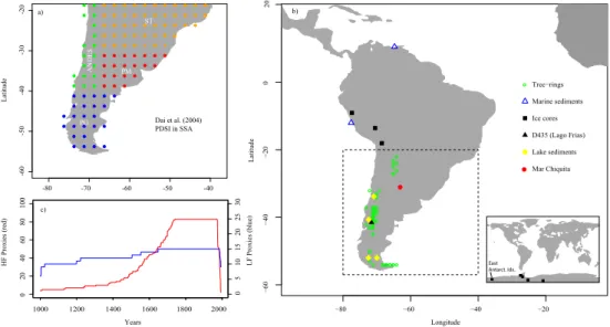
records in the area). The PDSI is a climatic metric that measures the departure from abnormally dry or wet condi-tions (relative to average local condicondi-tions). Three input vari-ables are required to calculate the PDSI: monthly precipi-tation, monthly temperatures, and the available water con-tent of soils. Within the calculation of the PDSI, moisture supply and demand are approximated in a simple hydrolog-ical accounting model that evaluates evapotranspiration, soil recharge, runoff, and moisture losses from the surface layer (see Palmer, 1965 for original equations). The PDSI pro-duces monthly indexes of meteorological droughts that ac-count for both contemporary and antecedent climatic condi-tions. The PDSI fluctuates between −10 (extremely dry) and +10 (extremely wet), with 0 corresponding to the local aver-age conditions. The PDSI should be regarded as an approxi-mation for dryness or wetness conditions rather than as an ab-solute value, as many factors like solar irradiation or aerosol concentrations are not considered explicitly. In the present paper, we use the gridded (2.5◦_×2.5◦_{) PDSI dataset}

com-puted by Dai et al. (2004) (Fig. 1a) and extended it to the last millennium in SSA. This dataset covers the 1870–2004 pe-riod and was calculated from long temperature (CRUTEM2, Jones and Moberg, 2003) and precipitation (Dai et al., 1997; Chen et al., 2002) series. We provide reconstructions of sum-mer (DJF) PDSI for each pixel in SSA. Sumsum-mer PDSI better integrates the effects of summer temperatures and precipita-tion along with lagged effects from previous seasons. We finally provide regional reconstructions for four regions sim-ilar to those identified by Neukom et al. (2010a) (Fig. 1a): Patagonia (PG), the Pampas (PM), Sub-Tropical SSA (ST), and the Andes (ANDES). Although climatic conditions and trends are not always uniform within these regions (e.g. PG, ANDES), the coarse source grid used here does not allow subdivision into smaller subsets.

2.2 Proxies

To achieve the PDSI reconstructions, we adopted a frequency-dependent approach similar to the one used by Moberg et al. (2005) where each proxy is used only to re-construct the periodicities for which it provides reliable in-formation (see Sect. 2.4 for details). A large proxy dataset

H F P roxi es (re d) L F P roxi es (bl ue ) a) -80 -70 -60 -50 -40 -60 -50 -40 -30 -20 PG PM ST A N D E S L at it ude Years Dai et al. (2004) PDSI in SSA

Figure 1. Proxy and PDSI data used in this analysis. Position of Dai et al (2004)’s 2.5 x 2.5 degrees PDSI in SSA

−80 −40 −20 −60 −40 −20 0 Tree−rings Marine sediments Ice cores D435 (Lago Frias) Lake sediments ● ●Mar Chiquita −60 1000 1200 1400 1600 1800 2000 0 20 40 60 80 100 0 5 10 15 20 25 30 L at it ude Longitude 20 b) c) East Antarct. Idx.

Fig. 1. Proxy and PDSI data used in this analysis. Position of Dai et al. (2004)’s 2.5 × 2.5 degrees PDSI in SSA (a). Location and type

of proxies used in this reconstruction (b). Evolution of the number of LF (0 < f < 0.08) and HF (0.08 < f < 0.5) series used for the reconstruction (c).

was compiled from high- and low-resolution proxies (Ta-ble 1, Fig. 1b,c). High-resolution proxies are mostly tree rings, most of which are available on the International Tree Ring Data Bank (ITRDB). We kept only the mean tree ring chronologies that were longer than 250 yr, giving a total of 82 tree ring predictors. In order to circumvent the well known problems associated with the standardization of tree ring series and the problematic interpretation of medium to low frequency variations (Esper et al., 2002, 2004), we re-tained only the high frequency variations conre-tained within these series. Low frequencies were removed in each tree ring chronology using a low-pass filter (based on the Fast Fourier Transform procedure). Basically, we removed all periodicities below a 12-yr threshold (f ≤ 0.08). In order to avoid the over-representation of tree ring series in the multi-proxy reconstruction, we selected (after infilling with the AM method, see next section) the first 7 PC explaining about 30 % of the variance of the high frequency tree ring series. Low-resolution proxies included marine sediments, lake sediments, and ice cores from the Andes and Antarc-tica (Table 1). The Fr´ıas sequence (Chapron, unpublished) is a new sedimentary record from a varved proglacial lake (Ariztegui et al., 2007) draining the Fr´ıas River Valley. The Fr´ıas sequence consists of a detailed record of goethite con-tent measured every 0.5 cm by sediment diffuse reflectance on a 187 cm long core retrieved in 2008 within Lago Fr´ıas main basin. The chronology (Fig. A1) has been established back to AD 1649 by varve counting on digital core images and by the identification of three mass wasting deposits in-duced by historical large earthquakes in AD 1960; AD 1751, and AD 1737. Geothite content in these annually laminated fine-grained sediments reflects soil erosion after rainfall.

2.3 Analogue method (AM)

The analogue method (Guiot et al., 2005) is commonly used to infill proxy-climate matrix containing missing values. The AM procedure aims at identifying, for each year i in the past where no PDSI value exists, the year k within the instrumen-tal record that has the most “similar” proxy vector. Here, similarity (d_ik2 ) is measured as an Euclidian distance (Guiot et al., 2005): d_ik2 =m−2_ik m X j =1 (xij−xkj)2 (xMj−xmj)2 δj_ik ! (1)

where xij represents the value of proxy j at year i, xkj

cor-responds to the value of proxy j at year k, M and m refer to the maximum and minimum value of the proxy j . δJ_ik is an index equal to 1 if a value is available for proxy j at year i and k, and equals 0 otherwise.

In the present paper, the AM was first used to infill both proxy and PDSI matrices (Fig. 2[1]). Since most available tree rings series terminated before ∼1993 (Table 1), we chose not to infill the proxy matrix up to the present in order to re-duce the possible bias associated with the use of an infilling method during the calibration period. Additionally, Dai et al. (2004)’s PDSI dataset presented some irregularities (in both mean and variance) before ∼1930 in SSA. These irreg-ularities are most likely associated with the very low number and poor quality of temperature and precipitation records in the early 20th century in that area. We therefore defined the 1930–1993 period for calibration. A total of 101 PDSI series were retrieved from Dai et al. (2004)’s dataset. We selected the first 12 PC explaining 77 % of the variance of the original PDSI series (Fig. 2[2]).

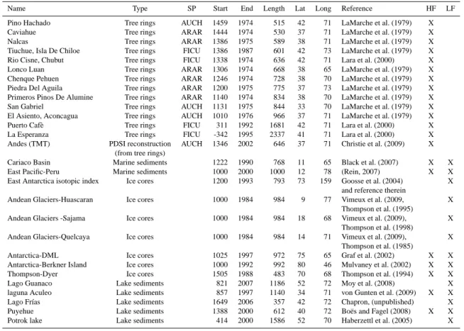
Table 1. The proxies used to reconstruct summer PDSI in SSA. HF = Proxies used to reconstruct the high frequency component (0.08 < f <

0.5). LF = Proxies used to reconstruct the low frequency component (0 < f < 0.08).

Name Type SP Start End Length Lat Long Reference HF LF

Lago Yehuin Tree rings NOPU 1731 1986 255 54 67 Boninsegna et al. (1989) X

Pampa Del Toro Tree rings AUCH 1736 1991 255 41 71 Villalba and Veblen (1997) X

Angostura Lago Alumine Tree rings ARAR 1717 1974 257 38 71 LaMarche et al. (1979) X

Pilcaniyeu Tree rings AUCH 1733 1991 258 41 70 Villalba and Veblen (1997) X

Estancia Carmen Camino T. Del Fuego Tree rings NOPU 1726 1986 260 54 67 Boninsegna et al. (1989) X

Puerto Parry T. Del Fuego Tree rings NOBE 1726 1986 260 54 64 Boninsegna et al. (1989) X

Estancia San Justo, T Del Fuego Tree rings NOPU 1723 1985 262 54 68 Boninsegna et al. (1989) X

Confluencia 2 Tree rings AUCH 1723 1989 266 37 71 Villalba and Veblen (1997) X

Bahia Crossley Isla De Los Estados Tree rings NOBE 1715 1986 271 54 65 Boninsegna et al. (1989) X

Paso De Las Nubes 3 Tree rings NOPU 1718 1991 273 40 71 Villalba et al. (1997) X

Rio Kilca Tree rings ARAR 1700 1974 274 38 70 LaMarche et al. (1979) X

Laguna Terrapien Tree rings AUCH 1700 1974 274 43 71 LaMarche et al. (1979) X

Lago Rucachoroi Tree rings AUCH 1700 1974 274 39 71 LaMarche et al. (1979) X

Lago Terraplen Tree rings AUCH 1700 1974 274 43 71 Villalba and Veblen (1997) X

Buenos Aires, Santa Cruz Tree rings NOPU 1706 1984 278 50 72 ITRDB series arge066 X

Rio Malenguena T. Del Fuego Tree rings NOPB 1705 1986 281 54 66 Boninsegna et al. (1989) X

El Maiten Tree rings AUCH 1690 1974 284 41 71 LaMarche et al. (1979) X

Estancia Harberton T. Del Fuego Tree rings NOBE 1700 1985 285 54 67 Boninsegna et al. (1989) X

Paso De Las Nubes 4 Tree rings NOPU 1701 1991 290 40 71 Villalba et al. (1997) X

Rio Bolsas, Piedra Parada,Jujuy Tree rings JUAU 1688 1981 293 23 65 Villalba et al. (1992) X

Monte Grande, Magallanes Tree rings NOPU 1677 1988 311 53 72 ITRDB series arge049 X

Volcan Lonquimay Tree rings ARAR 1664 1975 311 38 71 LaMarche et al. (1979) X

Paso Del Viento Tree rings AUCH 1679 1991 312 40 71 Villalba and Veblen (1997) X

Lago Quill`en Tree rings AUCH 1676 1989 313 39 71 Villalba and Veblen (1997) X

Aserradero Isla Grande T. Del Fuego Tree rings NOPB 1666 1986 320 54 67 Boninsegna et al. (1989) X

Estacion Microondas Tree rings NOPU 1664 1984 320 54 67 Boninsegna et al. (1989) X

Paso Gari Baldi Tree rings NOPB 1662 1985 323 54 71 Boninsegna et al. (1989) X

Lago Rucachoroi Tree rings ARAR 1650 1975 325 39 71 LaMarche et al. (1979) X

Peninsula Brunswick Tree rings NOPU 1662 1988 326 40 71 Boninsegna et al. (1989) X

El Chacay Tree rings AUCH 1650 1976 326 37 71 LaMarche et al. (1979) X

Copahue Tree rings ARAR 1640 1974 334 37 71 LaMarche et al. (1979) X

Paso Cordova, Neuquen Tree rings NOPU 1652 1986 334 40 71 ITRDB series arge050 X

Lago Fontana, Chubut Tree rings NOPU 1647 1985 338 45 71 ITRDB series arge037 X

Bahia York Tree rings NOBE 1647 1986 339 54 65 ITRDB series arge023 X

Aserradero Isla Grande Monticulo Tree rings NOPB 1639 1986 347 54 67 Boninsegna et al. (1989) X

Castano Overo Maduro Tree rings NOPD 1626 1982 356 41 71 ITRDB series arge027 X

El Mirador, Traful Tree rings AUCH 1635 1991 356 40 71 Villalba and Veblen (1997) X

Santa Isabel De Las Cruces Tree rings AUCH 1600 1970 370 34 70 LaMarche et al. (1979) X

Lago Moquehue Tree rings ARAR 1601 1974 373 38 71 LaMarche et al. (1979) X

Lago Tromen Tree rings ARAR 1600 1978 378 54 67 LaMarche et al. (1979) X

Glaciar Fr´ıas Tree rings NOPU 1595 1985 390 41 71 LaMarche et al. (1979) X

Estancia Collun-Co, Ca`oadon De Arriba Tree rings AUCH 1596 1989 393 39 71 Villalba and Veblen (1997) X

Estancia Pulmari Tree rings ARAR 1589 1989 400 39 71 LaMarche et al. (1979) X

Rio Minero Tree rings AUCH 1589 1991 402 40 71 Villalba and Veblen (1997) X

Lago Escondido Tree rings NOPB 1575 1984 409 54 67 Boninsegna et al. (1989) X

Casta`oo Overo 8 Tree rings NOPU 1572 1991 419 41 71 Villalba et al. (1997) X

Huinganco Tree rings AUCH 1550 1975 425 37 70 LaMarche et al. (1979) X

Nahuel – Pan Tree rings AUCH 1567 1992 425 42 71 Villalba and Veblen (1997) X

Norquinco Tree rings AUCH 1562 1989 427 39 71 Villalba and Veblen (1997) X

Casta`oo Overo 7 Tree rings NOPU 1562 1991 429 41 71 Villalba et al. (1997) X

Cuyin Manzano Tree rings AUCH 1543 1974 431 40 71 LaMarche et al. (1979) X

Piuchue, Isla De Chiloe Tree rings PIUV 1554 1987 433 33 70 Roig (1991) X

Estancia Teresa Tree rings AUCH 1540 1974 434 42 71 LaMarche et al. (1979) X

Cerro Los Leones Tree rings AUCH 1539 1974 435 41 71 LaMarche et al. (1979) X

Cerro Diego De Leon Tree rings NOPU 1546 1991 445 41 71 Schmelter (2000) X

Casta`oo Overo 6 Tree rings NOPU 1539 1991 452 41 71 Villalba et al. (1997) X

Rio Moat T. Del Fuego Tree rings NOBE 1528 1986 458 54 66 Boninsegna et al. (1989) X

Cerro La Hormiga Estancia Collun-Co Tree rings AUCH 1508 1989 481 40 71 Villalba and Veblen (1997) X

Puente Del Agrio Tree rings ARAR 1486 1974 488 42 71 LaMarche et al. (1979) X

Rahue Tree rings AUCH 1483 1974 491 39 70 LaMarche et al. (1979) X

Cerro Del Guanaco Tree rings AUCH 1497 1991 494 41 70 Villalba and Veblen (1997) X

Lago Quill`en Tree rings AUCH 1676 1989 495 40 71 Villalba and Veblen (1997) X

Caramavida Tree rings ARAR 1479 1976 497 34 70 LaMarche et al. (1979) X

Santa Lucia, Chiloe Continental Tree rings PIUV 1489 1986 497 43 72 Roig and Boninsegna (1992) X

Santa Lucia Tree rings PIUV 1489 1986 497 43 72 Roig and Boninsegna (1992) X

Table 1. Continued.

Name Type SP Start End Length Lat Long Reference HF LF

Pino Hachado Tree rings AUCH 1459 1974 515 42 71 LaMarche et al. (1979) X

Caviahue Tree rings ARAR 1444 1974 530 37 71 LaMarche et al. (1979) X

Nalcas Tree rings ARAR 1386 1975 589 38 71 LaMarche et al. (1979) X

Tiuchue, Isla De Chiloe Tree rings FICU 1386 1987 601 42 73 LaMarche et al. (1979) X

Rio Cisne, Chubut Tree rings FICU 1338 1974 636 42 71 Lara et al. (2000) X

Lonco Luan Tree rings ARAR 1306 1974 668 38 65 LaMarche et al. (1979) X

Chenque Pehuen Tree rings ARAR 1246 1974 728 38 70 LaMarche et al. (1979) X

Piedra Del Aguila Tree rings ARAR 1200 1975 775 37 73 LaMarche et al. (1979) X

Primeros Pinos De Alumine Tree rings ARAR 1140 1974 834 38 70 LaMarche et al. (1979) X

San Gabriel Tree rings AUCH 1131 1975 844 33 70 LaMarche et al. (1979) X

El Asiento, Aconcagua Tree rings AUCH 1010 1976 966 37 71 LaMarche et al. (1979) X

Puerto Caf`e Tree rings FICU 311 1992 1681 42 71 Lara et al. (2000) X

La Esperanza Tree rings FICU -342 1995 2337 41 71 Lara et al. (2000) X

Andes (TMT) PDSI reconstruction AUCH 1346 2002 646 37 71 Christie et al. (2009) X

(from tree rings)

Cariaco Basin Marine sediments 1222 1990 768 11 65 Black et al. (2007) X X

East Pacific-Peru Marine sediments 1000 2000 1000 12 78 (Rein, 2007) X X

East Antarctica isotopic index Ice cores 1200 1993 793 73 159 Goosse et al. (2004) X

and reference therein

Andean Glaciers-Huascaran Ice cores 1000 1984 984 9 77 Vimeux et al. (2009, X

Thompson et al. (1995)

Andean Glaciers -Sajama Ice cores 1000 1984 984 18 68 Vimeux et al. (2009), X

Thompson et al. (1998)

Andean Glaciers-Quelcaya Ice cores 1000 1984 984 14 71 Vimeux et al. (2009), X

Thompson et al. (1985)

Antarctica-DML Ice cores 1025 1997 972 75 65 Graf et al. (2002) X X

Antarctica-Berkner Island Ice cores 1000 1992 992 80 46 Mulvaney et al. (2002) X X

Thompson-Dyer Ice cores 1505 1988 483 70 68 Thompson et al. (1994) X X

Lago Guanaco Lake sediments 821 2007 1186 52 72 Moy et al. (2008) X

laguna Aculeo Lake sediments 857 1997 1140 34 71 von Gunten et al. (2009) X X

Lago Fr´ıas Lake sediments 1649 2006 357 42 72 Chapron, (unpublished) X

Puyehue Lake sediments 1388 2000 612 40 72 Bo¨es and Fagel (2008) X X

Potrok lake Lake sediments 414 2000 1586 52 70 Haberzettl et al. (2005) X

2.4 Spectral analogue method (SAM)

The reconstruction of the 12 PC of PDSI is also based on the AM, but it is performed separately for each frequency band using a spectral analogue method (SAM). The SAM (Guiot et al., 2010) is a combination of the AM with a spectral de-composition procedure that aims at achieving the reconstruc-tion separately for each frequency band (HF: high frequency band, LF: low frequency band). We defined the LF band as all periodicities below f = 0.08 (or T <12 yr, fixed by experimentation) and the HF band as all periodicities com-prised between 0.08 and 0.5 (12 yr > T > 2 yr). While it is assumed that all frequency bands are present in the PDSI se-ries (0 < f < 0.5), the SAM method allowed choosing, for each frequency band, which proxies are the most reliable predictors. The decomposition of both proxy and PDSI se-ries into their LF and HF component is achieved through a spectral decomposition algorithm (SD, Fig. 2[3]) based on the Fast Fourier Transform (FFT). The FFT first transforms each series into the frequency domain. Then, all frequen-cies outside the band are set to zero. Finally, the residual spectrum is back-transformed into the time domain using the inverse FFT. LF and HF bands are complementary be-cause their summation restitutes the original series. Thus,

for each frequency component, the AM is used to recon-struct the corresponding band of the PDSI PCs over the last millennium (Fig. 2[4]). The LF and HF bands of each PC are reconstructed independently from one another. Finally, the two bands are restituted into one single band (SR) and back-transformed into the original gridded PDSI data using an inverse PC (PC−1) procedure (Fig. 2[5,6]).

2.5 Uncertainty assessment

In the present paper, steps 4 to 6 on Fig. 2 were repeated iteratively (100 times here) and allowed for the implementa-tion of an h-block jackknife procedure (Guiot et al., 2010), which provided independent validation statistics and confi-dence intervals for the reconstructed values. At each iter-ation, a randomly selected year t was removed from each frequency band, and a training dataset defined after the ex-clusion of year t along with the four preceding and following years (h = 9). The AM was then used to predict the left-out year t from the training dataset in each band. This adaptation of the traditional jackknife method has proven to be partic-ularly useful with series (like LF series) that present a high degree of autocorrelation (Guiot et al., 2010). In our case, it forbade that the best analogue for year t could be found

+ + LF HF HF LF HF LF + PROXIES Reconstructed PDSI Observed PDSI AM [1] AM [1] PC [2] SD [3] SD [3] AM LF HF SR [5] PC-1

_[6]

Fig. 2. Summary of the spectral analogue method. Missing values in the proxy and summer PDSI matrix are filled with the analogue

method (AM[1]). The PDSI are reduced to m principal components. (PC [2]). Proxy and PDSI (PC) series are decomposed into their LF (0 < f < 0.08) and HF (0.08 < f < 0.5) components using a Fast Fourier Transform procedure (SD [3]). The reconstruction for each band is achieved using the AM [4]. This is done iteratively 100 times, and at each iteration, a random year t is removed for the calculation of validation statistics. Around year t , the [t − 4, t + 4] surrounding years are excluded as potential analogues. This h-block procedure is particularly useful in situations, like LF series, where there exists a large autocorrelation between years, causing the best analogues to be systematically located before of after year t. At each iteration, the reconstructed HF and LF bands are summed up to recompose (SR [5]) the full spectra of each PC. The PC are back-transformed into the original PDSI series using and inverse PC procedure (PC-1, [6]). The reconstructed series are finally verified against observations (Verification [7]).

between year t − 4 to t+4. An analysis of the autocorrela-tion structure within summer PDSI series revealed that the years located immediately outside the block had less than 30 % of variance in common with year t. Such an h-block jackknife procedure was performed 100 times with differ-ent randomly chosen years and allowed for the calculation of the RE statistic (Reduction of Error); a validation statis-tic (Fig. 2[7]) commonly used in dendroclimatology (Fritts, 1976). A check of the autocorrelation structure of residuals was also performed using the Durbin-Watson (DW) statistic (Durbin and Watson, 1950). Moreover, the information

pro-duced at each iteration allowed for the computation of 95 % confidence intervals around reconstructed values.

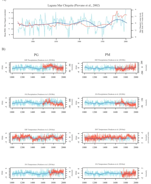
As a further validation for our reconstructions, we used a published sedimentological record of Mar Chiquita’s lake levels fluctuations (Piovano et al., 2002). Mar Chiquita is a large Sub-Tropical lake (about 6000 km2in size) that drains a vast area (about 127 000 km2). It is reasonable to assume that the fluctuations of such a vast hydrosystem are controlled by parameters (temperature and precipitation) that are sim-ilar to those that also influence summer PDSI in the area. Thus, this record might be adequate to evaluate the quality

1930 1940 1950 1960 1970 1980 1990 −4 −2 0 2 1930 1940 1950 1960 1970 1980 1990 −4 −2 0 2 1930 1940 1950 1960 1970 1980 1990 −3 −1 1 3 1930 1940 1950 1960 1970 1980 1990 −2 0 2 4 1930 1940 1950 1960 1970 1980 1990 −2 0 2 P D S I P D S I P D S I P D S I P D S I

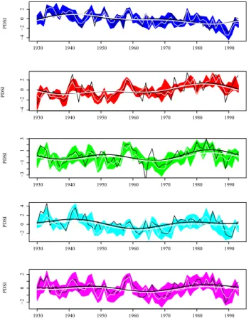
Figure 3. Comparison between observed (white) and reconstructed (black) summer PDSI series

Fig. 3. Comparison between observed (white) and reconstructed

(black) summer PDSI series for each region of SSA during the cal-ibration period (1930–1993). Bold lines are loess smoothings. The 95 % confidence intervals correspond to the colored zones. This color code will prevail in the next figures.

P D S I P D S I

LF (0 < f < 0.08)

HF (0.08 < f < 0.5)

Fig. 4. The 1930–1993 LF and HF components of the summer PDSI

in SSA. Observed and reconstructed values are in red and black, respectively.

Table 2. Mean calibration and validation statistics for each region

of SSA. Median values were averaged and the minimum and maxi-mum are given in parentheses.

Region R R2 RE DW PG 0.67 0.40 0.36 1.90 (0.57, 0.83) (0.21, 0.63) (−0.01, 0.56) (1.58, 2.30) PM 0.61 0.37 0.30 1.93 (0.46, 0.78) (0.17, 0.59) (0.01, 0.57) (1.67, 2.17) ST 0.65 0.39 0.30 1.96 (0.53, 0.76) (0.26, 0.56) (0.03, 0.49) (1.43, 2.44) ANDES 0.63 0.32 0.25 1.92 (0.53, 0.78) (0.19, 0.54) (−0.12, 0.56) (1.51, 2.37) SSA 0.64 0.37 0.30 1.93 (0.52, 0.78) (0.19, 0.58) (0.06, 0.55) (1.49, 2.36)

of our reconstruction, at least the long-term trends. Finally, despite the fact that a number of proxies are shared between the studies, we compared our PDSI reconstructions with the precipitation and temperature reconstructions of Neukom et al. (2010a, 2010b). This was done to analyze which climatic parameter (P or T ) is the best related, over time and space, to summer PDSI in SSA.

3 Results and discussion

3.1 Calibration and validation statistics of the SAM

The SAM yields satisfying results and suggests that the PDSI can be reconstructed in most areas of SSA. A good fit exists between observations and predictions for the full calibration period (1930–1993) (Fig. 3), and this fit is reasonably good in each frequency band (Fig. 4). The mean correlation coef-ficient (R) for SSA is 0.64 and ranges from 0.52 (minimum) to 0.78 (maximum) (Table 2) for the full spectra. The av-erage correlation coefficient is also very similar between the studied regions, with the lowest R value found in PM (0.61) and the highest in the PG region (0.67). On average, the SAM reconstructs about 37 % of the variance of the PDSI in SSA (Table 2). The percentage of variance accounted for by the model (coefficient of determination, R2) varied between 19 % and 58 %. Figure 5 shows the spatial distribution of these calibration statistics. In general, the relationships be-tween observations and predictions tend to be slightly weaker in the southern part of the Andes. A possible reason could be that the observed PDSI values might be less well estimated in this region of high climatological variability and altitudi-nal contrasts, a situation that would result in locally spurious trends. A second reason could be that the proxies themselves, although numerous in that area, do not cover the full range of variability within these pixels.

A property of the spectral analogues method, by compari-son to other regression-based methods, is to preserve a large

Distribution of R Distribution of R2 _{Distribution of RE}

Figure 5. Distribution of R, R2 _{and RE statistics in SSA. These calibration and validation statistics were}

caclcula-Fig. 5. Distribution of R, R2, and RE statistics in SSA. These calibration and validation statistics were caclculated on the full set of proxies,

and the data was interpolated with a thin-plate spline regression.

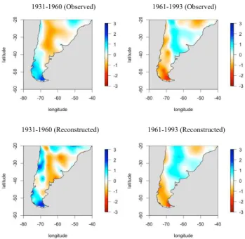
1931-1960 (Observed)

1931-1960 (Reconstructed) 1961-1993 (Reconstructed)

1961-1993 (Observed)

Fig. 6. Spatial comparison between observed (upper panel) and

re-constructed (lower panel) summer PDSI values for two contrasted

∼30 yr periods: 1931–1960 (left) and 1961–1993 (right).

amount of the original variance within the series if the refer-ence period is sufficiently diversified. In other words, when a regression technique is used, the proportion of reconstructed variance decreases with the R2. This attenuation effect be-comes even more exaggerated in the past because the number of proxies, and then the R2, diminishes with time. Yet spec-tral analogues are less sensitive to these effects since they are similarity-based and consequently they are able to reproduce all the variance contained in the reference period. To illus-trate this effect in SSA, we calculated the ratio of standard deviations between reconstructed and observed PDSI series in each region and observed that the former corresponds to

about 85 to 95 % of the latter. Therefore, we conclude that this property facilitates the analysis of extremes.

Validation statistics confirm the predictive skills of our model. RE is generally positive over SSA (Table 2), suggest-ing that the SAM provides better estimates of the PDSI than the climatology. Moreover, the DW statistic is always very close to 2, an indication that there is no significant first-order autocorrelation structure in the residuals (Durbin and Wat-son, 1950). The mean RE value was, on average, around 0.30 in all sub-regions except the Andes (0.25) but generally oscil-lated between 0 and 0.55 (taking into account the 95 % confi-dence intervals over all SSA). These performances are com-parable to the RE values obtained with the same method ap-plied in Europe to reconstruct growing season temperatures (Guiot et al., 2010). They are below the average RE (0.73) obtained by Neukom et al. (2010a) in a principal compo-nent reconstruction of summer DJF temperatures in SSA, but they are comparable to those found in the precipitation recon-struction (average RE around 0.27 in both seasons, Neukom et al., 2010b). Our RE values in the Mediterranean region of the Andes (around 0.35) are also comparable to the RE calculated by Christie et al. (2009) in a tree-ring reconstruc-tion of PDSI in this area (around 0.45). However, Christie et al. (2009)’s reconstruction focused on high frequencies, while our multi-proxy reconstruction aims at reconstructing the full spectra of PDSI variations. Therefore, the compar-ison between RE statistics should be interpreted with care, as errors propagate differently when HF and LF bands are reconstructed simultaneously.

The capacity of the SAM to reproduce modern spatial pat-terns of variations of the PDSI in SSA is another indication of the performance and usefulness of our modeling approach. Figure 6 presents the maps of the average observed and re-constructed PDSI values for two consecutive 30-yr windows (1931–1961 and 1961–1993). The first period (1931–1961) is marked by wet conditions in PG and the ANDES and a drier climate in PA and ST. This pattern is also very clearly

M ar Chi qui ta 's w at er l eve ls (di ff. from 1973 w at er l eve l) 1800 1850 1900 1950 2000 -4 0 2 4 -4 -2 0 2 4 -2 M ea n P D S I / M ar Chi qui ta w at ers he d

DJF Precipitation (Neukom et al. (2010b)) DJF Precipitation (Neukom et al. (2010b))

JJA Precipitation (Neukom et al. (2010b)) JJA Precipitation (Neukom et al. (2010b))

DJF Temperature (Neukom et al. (2010a)) DJF Temperature (Neukom et al. (2010a))

PG PM

Laguna Mar Chiquita (Piovano et al., 2002)

JJA Temperature (Neukom et al. (2010a)) JJA Temperature (Neukom et al. (2010a))

1000 1200 1400 1600 1800 2000 -3 0 3 50 -50 1000 1200 1400 1600 1800 2000 -3 0 3 -50 100 1000 1200 1400 1600 1800 2000 -3 0 3 -2 0 2 1000 1200 1400 1600 1800 2000 -3 0 3 -3 0 2 1000 1200 1400 1600 1800 2000 -4 0 4 -200 0 200 1000 1200 1400 1600 1800 2000 -4 0 4 -50 150 1000 1200 1400 1600 1800 2000 -4 0 4 2 0 -2 1000 1200 1400 1600 1800 2000 -4 0 4 -2 0 2 P D S I P D S I P D S I P D S I A nom al y A nom al y A nom al y A nom al y A nom al y (re ve rs ed s ca le ) A nom al y A nom al y A nom al y P D S I P D S I P D S I P D S I A) B)

Fig. 7. Comparison with (A) Mar Chiquita (Piovano et al., 2002) and (B) Neukom et al. (2010a, b) temperature and precipitation

reconstruc-tions. The summer PDSI reconstruction is always in blue, and the other works are in red. We present only the comparison for PG and PM to emphasize the contrasts. Bold (red and blue) lines represent 50 yr smoothings.

1000 1200 1400 1600 1800 2000

0.0

0.2

0.4

RE

Fig. 8. Evolution of RE statistics for the nested reconstructions in

each region of SSA. RE values were updated each time a new low frequency proxy was added to the reconstruction. Colors are the same as in Fig. 3.

seen in our reconstruction. The second period (1961– 1993) has the opposite pattern: a wet climate in PM and ST and drier conditions in PG and the ANDES. This spatial inver-sion of PDSI trends was well captured in our reconstruction. As an independent validation for our work, we checked the correspondence between our reconstruction and the 1767– 2002 reconstruction of Laguna Mar Chiquita water-levels fluctuation (Piovano et al., 2002). We used the average PDSI within the lake’s watershed for a comparison (60–65◦_{W; 20–}

25◦_{S). The agreement between the two series is fairly good}

(Fig. 7), at least in the mid to low frequency domains, consid-ering that both reconstructions were performed from totally independent proxies. The abrupt rise of Mar Chiquita’s lake

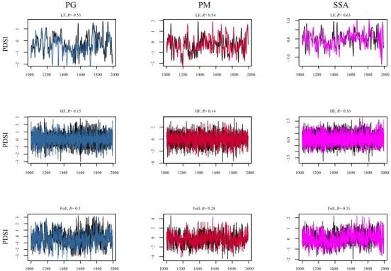
1000 1400 1800 −2 −1 0 1 LF, R= 0.53 −3 −1 1 2 3 HF, R= 0.15 −3 −1 1 2 3 Full, R= 0.3 −2 −1 0 1 2 LF, R= 0.54 −4 −2 0 2 HF, R= 0.14 −4 −2 0 2 4 Full, R= 0.28 −1.0 0.0 1.0 LF, R= 0.63 −1.5 0.0 HF, R= 0.16 −2 −1 0 1 2 Full, R= 0.31 1200 1600 2000 1000 1200 1400 1600 1800 2000 1000 1200 1400 1600 1800 2000 1000 1200 1400 1600 1800 2000 1000 1200 1400 1600 1800 2000 1000 1200 1400 1600 1800 2000 1000 1200 1400 1600 1800 2000 1000 1200 1400 1600 1800 2000 1000 1200 1400 1600 1800 2000 PG PM SSA P D S I P D S I P D S I 0 −2 0 −2 1.5

Fig. 9. Comparison between the reconstructions made from the full proxy dataset (colored lines, same colors as in Fig. 3) and the

reconstruc-tions performed from only the proxies that go back to AD 1000 (black lines). The top and middle rows present the LF and HF components, respectively, while the lower row depicts the comparison over the full spectra. Correlation coefficients (R, N = 994) are shown in the title, for each frequency band and for each region. Not shown here: ANDES (R = 0.28, for the full spectra) and ST (R = 0.57, for the full spectra).

levels during the 1970s also corresponds to a rise in summer PDSI, although the latter has a smaller amplitude. It is worth mentioning that a recent modeling of Mar Chiquita’s water levels has shown that the recent rise is attributable to an in-crease in runoff in the northern sub-basin (Troin et al., 2010), evoking an increasingly dominant tropical influence in the area. Thus, since the PDSI is a value that is standardized to reflect departures from local mean conditions, the average PDSI within the mar Chiquita watershed may not adequately reflect this possible flow redistribution.

Before exploring millennial summer PDSI fluctuations, it is important to establish that our reconstruction is reli-able over the full period. To do so, we provide a series of nested reconstructions and their corresponding verifica-tion (RE) statistics. Nested reconstrucverifica-tions were computed exclusively from subsets of proxies that are older than AD: 1000, 1025, 1200, 1222, 1388, 1505, 1649 respectively cor-responding to the calendar dates to which a new LF proxy is added to the reconstruction. We present the evolution of RE statistics in each sub-region on Fig. 8. Even with a limited number of proxies at the beginning of the last millennium, the RE statistics remains positive in all regions, meaning that the spectral analogues have good predictive skills over the last thousand years. As an example, we graphically com-pare the full reconstruction and the AD 1000 nested recon-struction (Fig. 9) for two regions: PG and PM. Our analysis

shows that LFs are comparable between reconstructions over the last thousand years. However, HFs are less similar and this probably relates to the fact that higher frequencies con-tain a lot of the local climatic signal (i.e. noise) that cannot be adequately reconstructed from a very limited number of HF proxies. In conclusion, the correlations for the full spectra remain acceptable, suggesting that the long-term trends can be interpreted since AD 1000.

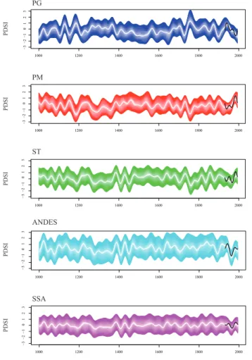
3.2 PDSI fluctuations over the last millennium in SSA

Summer PDSI reconstructions (1000–1993) and regime shift detection analysis (extended until AD 2005 using Dai et al. (2004)’s PDSI data) are presented in Figs. 10 and 11. The period between 1000 and ∼1250 clearly appears as a distinct regime in all areas of SSA. Breakpoints correspond-ing to the end of the latter period were identified in 1242 (PG) 1241 (PM), 1234 (ST), and 1255 (ANDES) (Fig. 11). In most regions except PG, the first part of the millennium was probably slightly wetter that today. This period cor-responds to the end of the MWP that extended until 1200– 1350 in the Northern Hemisphere (Jansen et al., 2007; Mann et al., 2009; Guiot et al., 2005, 2010; DahlJensen et al., 1998), and until about 1200–1250 in the Southern Hemi-sphere (Cook et al., 2002). In SSA, the MWP seemed to have persisted until about ∼1350 (Neukom et al., 2010a). The

1000 1200 1400 1600 1800 2000 1000 1200 1400 1600 1800 2000 −3 −1 1 2 3 1000 1200 1400 1600 1800 2000 1000 1200 1400 1600 1800 2000 1000 1200 1400 1600 1800 2000 PG PM ST ANDES SSA 0 −2 −3 −1 1 2 3 0 −2 −3 −1 1 2 3 0 −2 −3 −1 1 2 3 0 −2 −3 −1 1 2 3 0 −2

Millennial summer PDSI reconstructions for each region of SSA. 30-year -ment). The color code is the same as in Figure 3.

P D S I P D S I P D S I P D S I P D S I

Fig. 10. Millennial summer PDSI reconstructions for each region

of SSA. 30-yr filtered chronologies are presented. Observations are in black and reconstructions are in white. Colored shadings corre-spond to 95 % confidence intervals (darker at each 5 % increment). The color code is the same as in Fig. 3.

100-yr lag between our PDSI reconstruction and Neukom et al. (2010a) summer temperature reconstruction needs fur-ther investigation but could possibly be explained by changes in precipitation patterns that are not present in temperature reconstructions. It is interesting to note, however, that from the perspective of PDSI, the first part of the millennium in SSA was probably a period of important geographical con-trasts rather than a widespread drought.

The ∼1250–∼1380 period is also clearly distinct in all re-gions of SSA and is characterized by drier than normal con-ditions (Figs. 10 and 11), except in PG where wetter condi-tions prevailed. Again, regime-ending dates cluster in time: 1376 (PG), 1375 (PM), 1386 (ST), 1384 (ANDES), and 1369 (SSA). Interestingly, this well-defined regime corresponds to the Wolf Minimum (Eddy, 1976), the first period of the LIA with an extremely low solar activity. The physical link be-tween solar irradiation and the PDSI in SSA, however, needs to be substantiated by modeling studies in order to clarify the processes and forcings involved. Additionally, the possible climatic impact of volcanic eruptions should be investigated,

P roport ion −4 −2 0 2 4 −4 −2 0 2 4 −4 −2 0 2 4 −4 −2 0 2 4 −4 −2 0 2 4 1000 1200 1400 1600 1800 2000 0.00 0.10 0.20 P D S I P D S I P D S I P D S I P D S I PG PM ST ANDES SSA

Proportions of series with a change date (20 yr running average)

Fig. 11. Regime shift detection in summer PDSI series in SSA.

The analysis was performed using the Rodionov (2004) method. Regime shift detection is based on a sequential a t-test algorithm.To be detected, a regime needs to be at least 50 yr long. If a regime has less than 50 yr, the method can still allow for its detection; however, the significance required to determine that a date corresponds to a changepoint is adjusted to be inversely related to the length of the regime. The bottom panel corresponds to the 20 yr running proportion of the number of series, recording a changepoint at year

t . It gives a general idea of where these changepoints cluster in

time. Color code from Fig. 3 is used here.

as a series of major eruptions occurred during that period (Wanner et al., 2008). The physical processes driving these changes are currently being examined through a model-data comparison study.

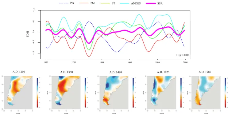
968 E. Boucher et al.: A millennial multi-proxy reconstruction of summer PDSI´ P D S I PG PM ST ANDES SSA 0 < f < 0.02 ≤ 0.02). Example maps 1000 1200 1400 1600 1800 2000 −1.0 −0.5 0.0 0.5 −1.0

≤ 0.02). Example maps

A.D. 1200 A.D. 1350 A.D. 1480 A.D. 1825 A.D. 1980

Fig. 12. Smoothed summer PDSI reconstruction for each region of SSA emphasizing the antiphase between SP and the rest of the continent.

Smooth lines correspond to 50-yr low pass filters (f ≤ 0.02). Example maps of 30-yr periods centered on AD 1200, 1350, 1690, 1825, and 1980 are shown.

The 1780–1820 is also an important regime change period (Figs. 10 and 11) and corresponds to the Dalton minimum (Eddy, 1976), though its spatial extent is less marked that the two previously described periods. Wetter than normal conditions were recorded in PG, while drier conditions were reconstructed in PM and ST.

Although important regime changes occurred over the last centuries, most fell within the bounds of the last millennium variability (Fig. 11). The best example is the drying episode that occurred in PG since ∼1880. Similar regime conditions could be found between 1400 and 1750 in the area, and even before ∼1250. We must point out that, while individual years within the regimes are reconstructed by analogy using the SAM, regimes drier or wetter than today can actually be re-constructed if, for example, extreme years (either wet or dry) cluster in a given past period. This was rarely the case in our analysis. Nevertheless, several exceptions exist. The recent wet regime in PM seems rare (if not exceptional) at the scale of the last millennium; so is the dry regime observed in the ANDES since the 1930s that has very few (if no) equivalent in the past.

A striking feature of our reconstruction is an antiphase be-tween PG and the rest of the subcontinent. A comparison of 50-yr-filtered reconstructions (Fig. 12) reveals that SSA’s summer PDSI evolution, rather then being uniform over all the studied area, was characterized by an important geo-graphical contrast, especially between the northeast and the southernmost part of the continent. That contrast can be most

easily perceived in the low frequency domain (f < 0.03), but it characterizes, typically, all frequency bands below 0.2 (T = 5yr). In order to better interpret that antiphase, we com-pared our reconstructions of contrasted PG and PM regions to those of Neukom et al. (2010a and 2010b) (Fig. 7). In PG, summer PDSI seemed to be more responsive to temperatures than to precipitation. In this area, warm summers and winters were associated with a wet climate (positive relationship). By contrast, in PM, PDSI seemed closely linked to DJF pre-cipitation. Moreover, DJF and JJA temperatures related dif-ferently to summer PDSI. Warm summers were associated with a dry climate while warm winters were generally cou-pled to wet summer conditions. These contrasting dynamics underline the fact that the PDSI might not have responded similarly to precipitation or temperature in every region, but instead that variations in the drought index were probably driven by different parameters whose importance are likely to vary through space.

A frequency analysis was performed to determine whether or not extremely wet (or dry) spells have been more common (or rarer) in the past. For each region, a reference PDSI value was defined. That value corresponded to the 50-yr wet spell and drought identified for the 1930–1993 period. Then, past return periods  ( = 1/probability to exceed the reference PDSI value) were retrieved after fitting a log-normal distri-bution to the 100 yr preceding each year t. The results are presented on Fig. 13 along with their bootstrap confidence intervals. Events equivalent in magnitude to the reference

5e 1 5e 3 1200 1400 1600 1800 2000 5e 1 5e 1 5e 2 5e 1 5e 2 1200 1400 1600 1800 2000 5e 4 5e 2 5e 1 5e 3 5e 4 5e 2 5e 1 5e 3 5e 4 5e 2 5e 1 5e 3 5e 2 5e 1 5e 3 5e 4 5e 2 5e 1 5e 3 5e 2 5e 1 5e 3 5e 4 5e 2 5e 5 5e 2 Re turn P eri ods (Ω , ye ars ) PG (ref=2.6) PM (ref=3.2) ST (ref=2,7) ANDES (ref=3.2) SSA (ref=1.9) PG (ref=-2.8) PM (ref=-3.2) ST (ref=2.4) ANDES (ref=2.8) SSA (ref=1.7)

. Past return periods (Ω) (and their 95% bootstrap confidence interval) of events equivalent in magnitude to the reference 50-yr wet spell (left panel) or drought (right panel). The reference 50-yr event (value indicated in parenthesis for each region) was calculated for the 1930-1993 period. All return periods were obtained after fitting a log-normal distribution to the 100 years preceding year . Color codes for each region are the same as in Figure 3. Return period values on the y axis are exponential values ie. 5e years =5*10 years. Thus values of 1,2 and 3 respectively yield 50-yr, 500-yr and 5000-yr return periods. Confidence intervals are incremented at each 5%, with reversed color directions for wet spells and droughts.

Fig. 13. Past return periods () (and their 95 % bootstrap

confi-dence interval) of events equivalent in magnitude to the reference 50-yr wet spell (left panel) or drought (right panel). The reference 50-yr event (value indicated in parenthesis for each region) was cal-culated for the 1930–1993 period. All return periods were obtained after fitting a log-normal distribution to the 100 yr preceding year t . Color codes for each region are the same as in Fig. 3. Return period

values on the y axis are exponential values i.e. 5ek years = 5 × 10k

years. Thus k values of 1, 2 and 3 respectively yield 50-yr, 500-yr and 5000-yr return periods. Confidence intervals are incremented at each 5reversed color directions for wet spells and droughts.

50-yr wet spell generally had a larger  between 1250 and 1400 ( > 500 yr), except in PG where their  was closer to the modern value ( ∼100 yr). Between 1400 and 1600, a tendency towards shorter  (<100 yr) can be observed ev-erywhere except in PG where very rare occurrences are noted ( > 500 yr). From 1600 to the 20th century, wet events progressively became more common, except in PM where they were rarer. The latter tendency reversed after 1900 in some regions: the ANDES (wet spells were rarer after 1970), PM (wet spells were more common after 1970), and PG (wet spells were rarer after 1900).

The frequency analysis of droughts revealed the antiphase as well (Fig. 13). In general, extreme droughts were com-mon before 1400 in most regions ( < 100 yr), except in PG where they were clearly rarer between 1250 and 1400 ( > 500 yr). Between 1450–1700, extremely dry events were rarer than today ( > 500 yr) almost everywhere in SSA, except in PG where an opposite trend can be observed. An interesting point is that although the antiphase between PG and SSA seems symmetrical for both droughts and wet spells, the behaviour of droughts with respect to their wet

spell counterparts is not necessarily symmetrical in each re-gion, possibly indicating a relative independency between the two phenomena. A good example of that independency is found in PM after 1400. While wet spells became less fre-quent in PM during that period (possibly indicating drier con-ditions in the area), extreme droughts also became less fre-quent between 1400 and 1600. Afterwards, severe droughts in PM became more common (20 <  < 100 yr) until about 1900, while wet spells were still quite rare (200 <  < 1000). This asymmetry highlights the fact that, regardless of the long-term trends in the mean of summer PDSI series, ex-tremely dry and/or wet spells can still occur isolatedly in small clusters and independently from the regime conditions. In other words, the driest (wettest) years do not systemati-cally occur during the driest (wettest) regimes.

3.3 Links with ocean-atmosphere forcings (AAO, ENSO, PDO)

The climate of SSA is under the influence of high latitude and tropical ocean-atmospheric forcings, but the magnitude and the direction of this influence varies considerably between regions. To explore the teleconnections between summer PDSI and the dominant indices in the area (summer means for AAO, ENSO, and PDO, all retrieved from the Climate Di-agnostics Center (NOAA) at http://www.esrl.noaa.gov/psd/ data/), we first used standard Pearson correlation analysis. The AAO index is estimated by the first PC of the 850 hPa geopotential height anomalies south of 20◦_{S (Thompson and}

Wallace, 2000). The ENSO index corresponds to the mean SST anomalies from the N3.4 Pacific region and is a com-mon proxy for the ENSO phenomenon (Trenberth, 1997). The PDO (Zhang et al., 1997) is an ENSO-like phenomenon that exhibits decadal to interdecadal variability (at least 20 to 30 yr). The estimation of the PDO interdecadal variabil-ity remains poorly known because very few stations in South America are century-long. In order to evaluate our recon-struction’s ability to reproduce climatic patterns driven by the major indices in SSA, reconstructed PDSI values were used as predictands. However, we also tested the relation-ships with instrumental PDSI values and the results are com-parable (Fig. 14).

Over the common period (1950–1993), AAO is well cor-related to summer PDSI in SSA. In PG and the ANDES, the correlation is negative and reaches R = −0.53, while in PM and ST, the correlation is positive (Fig. 14) and reaches R = 0.5. Thus, over the last 50 yr, AAO fluctuations have been associated with important climatic contrasts in SSA. Positive AAO indices are clearly associated with wet con-ditions in western PM and ST and with dry concon-ditions in PG and the ANDES. Negative AAO values show the opposite trend: wet PG and dry PM/ST. This latitudinally contrasted response of summer PDSI to the AAO might have some important implications for the interpretation of millennial PDSI trends in SSA. We showed earlier that low-frequency

AAO ENSO PDO

Fig. 14. Correlations (1950-1993) of reconstructed summer PDSI with the main ocean-atmosphere indices:

AAO, ENSO, and PDO.

AAO ENSO PDO

Correlations with reconstructed PDSI values

Correlations with Dai et al. (2004) PDSI values

Fig. 14. Correlations of reconstructed (upper panel) and Dai et al. (2004) (lower panel) summer PDSI with the main ocean-atmosphere

indices: AAO, ENSO, and PDO. All correlations were computed on the common 1950–1993 period.

variations (Fig. 12) and trends in the extremes (Fig.13) of summer PDSI in PG have been in antiphase with those on the rest of the sub-continent. It is now possible to argue that these antiphases could have been driven by past low-frequency variations in the AAO, since this index is the only one that can be associated to such a contrasted PDSI re-sponse. As underlined by Garreaud et al. (2009), the AAO is the leading pattern of tropospheric circulation variability south of 20◦_{S. Its influence on temperature over the recent}

period is unequivocal over the recent period (Gillett et al., 2006; Garreaud et al., 2009). The most striking aspect is a contrasted response of annual surface temperatures with a clear summer warming south of 40◦_{S and a cooling}

else-where during positive phase of the AAO (Garreaud et al., 2009). These results highlight the fact that summer PDSI variations in SSA are responsive to AAO-induced tempera-ture fluctuations at the continental scale, a result that is also supported by the comparison with Neukom et al. (2010a)’s temperature reconstruction.

Summer PDSI is also related to the ENSO phenomena in SSA (1951–1993). However, the response is far less

con-trasted than with AAO and mostly positive throughout the studied area (Fig. 14). The strongest correlations are found in the Mediterranean area of the Andes and along the eastern part of Argentina. Positive (negative) ENSO years typically generate conditions that are wetter (drier) that the normal in SSA. PDO is also related to the fluctuations of summer PDSI (1930–1993). This index has a general positive influence, but the highest correlations (R = 0.5) are found in the Mediter-ranean Andes region. Much like with ENSO, positive (neg-ative) PDO years generate conditions that are wetter (drier) than the normal almost everywhere in SSA.

Finally, it is clear that all these ocean-atmosphere forc-ings act synergically to influence summer PDSI in SSA. In order to better understand the interactions between AAO and ENSO, model-data comparison studies will be neces-sary. Here, we simply underline the fact that SSA’s summer PDSI can be compartmentalized according to the dominant ocean-atmosphere forcing. To determine which index has a predominant influence over the 1950–2005 period, we per-formed a regression analysis using each index as a predic-tor. For each 2.5◦_×2.5◦_{pixel in SSA, the equation had the}

ENSO (+/-) AAO (+/-) PDO (+/-) Dominant influence: Longitude L at it ude −80 −70 −60 −50 −40 −60 −50 −40 −30 −20

Fig. 15. Map of the magnitude and direction of the

dom-inant influence, (measured as the magnitude and sign of

the largest regression coefficient in the following equation: PDSI = a(AAO) + b(ENSO) + c(PDO)). Red symbols represent a dominant AAO influence while blue and green symbols indicate a dominant ENSO or PDO influence, respectively. Filled (empty) squares denote a positive (negative) influence on summer PDSI. The regression was performed for the longest common period (1950– 1993). Spots with no symbols had a negative RE value.

form PDSI = a(AAO) + b(ENSO) + c(PDO) + noise, where a, b, and c are coefficients. For each regression, we retained the largest coefficient (absolute value) and noted its sign (Fig. 15). Interestingly, this figure clearly shows that the var-ious regions of SSA are under the influence of different dom-inant indexes. In PG and northeastern ST, the domdom-inant pro-cess is clearly the negative and spatially coherent influence of AAO. A positive influence of AAO is also dominant west of 70◦_{W in PM and in lower ST. Both PDO and ENSO are both}

dominant in the Mediterranean ANDES, in western PM, and in ST. The dominant influences appear to be spatially coher-ent (points with a common influence tend to cluster in space), suggesting a true physical link between PDSI variations and these atmospheric circulation modes. The question remains whether or not these influences have been stationary through time and how did they interacted through time. Data-model comparison studies over the whole millennium are necessary to clarify these issues.

4 Conclusions

This study presents the first spatially explicit summer PDSI reconstruction in the Southern Hemisphere. We provide a 2.5◦_×2.5◦ _{gridded reconstruction that extends the Dai et}

al. (2004) PDSI dataset over the last millennium at the sub-continental scale, south of 20◦_{S in SSA. Calibration and}

ver-ification statistics, along with the spatial analysis of modern patterns of changes, show that in most areas of SSA (PG, PM, ST, ANDES), the summer PDSI is well reconstructed using the SAM. Over the last millennium, SSA has experi-enced considerable PDSI variations, some of which might have been at least as important as those recently observed in the area. The temporally well-defined 1000–1250 period possibly associated with the MWP was characterized by wet-ter than normal conditions in most studied regions, except in PG where the climate was clearly drier that the normal. This regime terminated very abruptly around ∼1250, as indicated by the regime shift detection and the analysis of extremes.

In most regions, the climatic spatial pattern reversed be-tween 1250 and ∼1400. SSA’s climate became much drier, except in PG where the climate humidified during the austral summer. Afterwards, SSA slowly humidified to approach conditions somewhat closer to the normal (although with some important discrepancies between regions, e.g. in PM the climate dried up).

The analysis of recent PDSI fluctuations in the context of the last millennium reveals analogous patterns for the mod-ern period over the last thousand years, especially between 1000 and 1400. Our reconstruction also shows that PG’s fluctuations were generally in antiphase with the rest of the continent. Such an antiphase could be driven by the Antarc-tic Oscillation (AAO), providing that modern patterns of re-sponse are transferable to the past. We reveal evidences that the AAO has a contrasted effect on the PDSI in SSA over the calibration period. During its positive phase, the climate tends to be humid in the northeastern part of SSA and much drier in the south. During its negative phase, the latter situa-tion reverses. However, AAO has never acted alone to mod-ulate fluctuations in the mean and extremes of PDSI. Never-theless, in some regions like PG, AAO clearly is the domi-nant driver (at least during the calibration period), while in others it plays a smaller role.

Our analysis finally shows that past low-frequency PDSI variations can be reconstructed quite successfully in most re-gions of SSA. We have shown that even with a reduced num-ber of proxies, low frequencies reconstructed using the SAM remain quite similar to the low frequencies reconstructed from the full dataset. However, we have also shown that high frequency PDSI variations are less well reconstructed from a reduced set of proxies. In order to better reconstruct high frequency variations of PDSI in SSA, more highly resolved proxies are needed, as stated by Villalba et al. (2009), es-pecially in proxy-lacking areas such as ST area and eastern PM.

Finally, future analysis should focus on studying the in-teractions between ocean-atmosphere forcings (e.g. interac-tions between AAO an ENSO) in order to better identify how they can modulate SSA’s climate in both time and space. Such work should preferentially be achieved through climate models.

G oe thi te c ont ent i n L ago F ri as S edi m ent s F irs t D eri va ti ve V al ue (445 nm ) 0.05 0.04 0.03 0.02 2000 1950 1900 1850 1800 1750 1700 1650 1600

-Fig. A1. Goethite (derivative 445 nm) chronology of Lago Fras

varved lake sediments. Stars represent some well-known earth-quakes in the area (AD 1960; AD 1751, and AD 1737).

Appendix A

A Complementary figure

Figure A1 represents the Goethite (derivative 445 nm) varved chronology of Lago Fr´ıas sediments (1645–2008). This sed-imentary proxy reflects the amount of precipitation-induced erosion in the watershed. The dating of these sediments was confirmed by three well-known earthquakes (1737, 1751, and 1960) also shown on the figure.

Acknowledgements. This paper is a contribution to the ESCARSEL

project funded by the French National Agency of Research (pro-gram VMC, project ANR-06-VULN-010). We also thank the post-doctoral fellowship program of the FQRNT (Fonds Qu´e`ıb´ecois de Recherche sur la Nature et les Technologies) that provided the grant to the first author. The comments from the two reviewers (R. Neukom and R. Villalba) and the editor (M. Masiokas) were much appreciated and contributed to improving the content of this manuscript. Dai Palmer Drought Severity Index data was provided by the NOAA/OAR/ESRL PSD, Boulder, Colorado, USA, and downloaded from their Web site at http://www.esrl.noaa.gov/psd/. Francoise Chali´e, Edouardo Piovano Francoise Vimeux, Florence Sylvestre, Raphael Neukom, E. M. Thompson, B. Rein, Dun-can Christie, Nathalie Fagel, Marie-France Loutre, Xavier Bo¨es, Chistopher Moy, Christophe Corona, Myriam Khodri, Francisco Da Cruz, Georg Hoffmann provided data and/or helpful discussions. The publication of this article is financed by CNRS-INSU. Edited by: M. H. Masiokas

The publication of this article is financed by CNRS-INSU.

References

Apipattanavis, S., McCabe, G. J., Rajagopalan, B., and Gangopad-hyay, S.: Joint spatiotemporal variability of global sea surface temperatures and global Palmer Drought Severity Index values, J. Climate, 22, doi:10.1175/2009JCLI2791.1171, 6251–6267, 2009.

Ariztegui, D., Bosch, P., and Davaud, E.: Dominant ENSO frequen-cies during the Little Ice Age in Northern Patagonia: the varved record of proglacial Lago Fr´ıas, Argentina, Quatern. Int., 161, 46–55, doi:10.1016/J.Quaint.2006.10.022, 2007.

Black, D. E., Abahazi, M. A., Thunell, R. C., Kaplan, A., Tappa, E. J., and Peterson, L. C.: An 8-century tropical Atlantic SST record from the Cariaco Basin: baseline variability, twentieth-century warming, and Atlantic hurricane frequency, Paleoceanography, 22, PA4204, doi:10.1029/2007PA001427, 2007.

Bo¨es, X. and Fagel, N.: Relationships between southern Chilean varved lake sediments, precipitation and ENSO for the last 600 years, J. Paleolimnol., 39, 237–252, 2008.

Boninsegna, J. A., Villalba, R., Amarilla, L., and Ocampo, J.: Stud-ies on tree rings, growth- rates and age-size relationships of trop-ical tree species in Misiones, Argentina, Iawa Bull., 10, 161–169, 1989.

Boninsegna, J. A., Argollo, J., Aravena, J. C., Barichivich, Christie, D. J., Ferrero, M. E., Lara, A., Le Quesne, C., Luckman, B. H., Masiokas, M., Morales, M., Oliveira, J. M., Roig, F., Srur, A., and Villalba, R.: Dendroclimatological reconstructions in South America: a review, Palaeogeogr. Palaeoecol., 281, 210– 228, 2009.

Bradley, R. S. and Jones, P. D.: “Little Ice Age” summer tempera-ture variations: their natempera-ture and relevance to recent global warm-ing trends, Holocene, 3, 367–376, 1993.

Briffa, K. R., Osborn, T. J., Schweingruber, F. H., Jones, P. D., Shiyatov, S. G., and Vaganov, E. A.: Tree-ring width and density data around the Northern Hemisphere: Part 1, local and regional climate signals, Holocene, 12, 737–757, 2002.

Chen, M., Xie, P., Janowiak, J. E., and Arkin, P. A.: Global land precipitation: A 50-yr monthly analysis based on gauge observa-tions, J. Hydrometeor., 3, 249–266, 2002.

Christie, D. A., Boninsegna, J. A., Cleaveland, M. K., Lara, A., Le Quesne, C. M. S. M., Mudelsee, M., Stahle, D. W., and Villalba, R.: Aridity changes in the Temperate-Mediterranean transition of the Andes since AD 1346 reconstructed from tree-rings, Clim. Dynam., 36(7–7), 1505–1521, doi:10.1007/s00382-009-0723-4, 2009.

Cook, E. R., Meko, D. M., Stahle, D. W., and Cleaveland, M. K.: Drought reconstructions for the continental United States, J. Cli-mate, 12, 1145–1162, 1999.

Cook, E. R., Palmer, J. G., and D’Arrigo, R. D.: Evidence for a Medieval Warm Period in a 1100 year tree-ring reconstruction of past austral summer temperatures in New Zealand, Geophys. Res. Lett., 29, 1667, doi:10.1029/2001gl014580, 2002. Cook, E. R., Woodhouse, C. A., Eakin, C. M., Meko, D. M., and

Stahle, D. W.: Long-term aridity changes in the Western United States, Science, 306, 1015–1018, doi:10.1126/science.1102586, 2004.

DahlJensen, D., Mosegaard, K., Gundestrup, N., Clow, G. D., Johnsen, S. J., Hansen, A. W., and Balling, N.: Past temperatures directly from the Greenland Ice Sheet, Science, 282, 268–271, 1998.